An improved estimate of inorganic iodine emissions from the ocean using a coupled surface microlayer box model

Iodine at the ocean's surface impacts climate and health by removing ozone (O₃) from the troposphere both directly via ozone deposition to seawater and indirectly via the formation of iodine gases that are released into the atmosphere. Here we present a new box model of the ocean surface microlayer that couples oceanic O₃ dry deposition to inorganic chemistry to predict inorganic iodine emissions. This model builds on the previous work of Carpenter et al. (2013), improving both chemical and physical processes. This new box model predicts iodide depletion in the top few micrometres of the ocean surface due to rapid chemical loss to ozone competing with replenishment from underlying water. From this box model, we produce parameterized equations for HOI and I₂ emissions, which are implemented into the global chemical transport model GEOS-Chem along with an updated sea surface iodide climatology. Compared to the previous model, inorganic iodine emissions from some tropical waters decrease by as much as half, while higher-latitude emissions increase by a factor of ≫10. With these large local changes, global total inorganic iodine emissions increased by ∼49 % (2.99 to 4.48 Tg) compared to the previous parameterization. This results in a negligible change in average tropospheric OH (<0.2 %) and tropospheric methane lifetime (<0.2 %). The annual mean tropospheric O₃ burden decreases (−1.5 % to 325 Tg); however, higher-latitude surface O₃ concentrations decrease by as much as 20 %.

1 Introduction

Iodine in the atmosphere and at the ocean–atmosphere interface is a large sink for tropospheric ozone (O₃). Dry deposition of O₃ to the ocean was thought to account for approximately one-third of the total O₃ loss to dry deposition (Ganzeveld et al., 2009); however, more recent work using more advanced representations of oceanic ozone dry deposition has revised this contribution down to ∼15 % (Luhar et al., 2018; Pound et al., 2020). At the ocean surface, the reaction between O₃ and iodide (I⁻) is thought to represent a significant fraction of this loss (Fairall et al., 2007; Carpenter et al., 2013). Most global models have a simplistic representation of oceanic O₃ dry deposition, which contributes to the uncertainty in tropospheric O₃ (Ganzeveld et al., 2009; Hardacre et al., 2015). Including a more advanced oceanic dry-deposition scheme that incorporates the chemical loss of O₃ to I⁻ and the physical processes that control O₃ dry deposition has been shown to improve model comparisons to observations of both oceanic dry-deposition velocity and remote marine surface O₃ concentrations (Luhar et al., 2017, 2018; Pound et al., 2020).

Photochemical cycling of iodine in the atmosphere leads to efficient chemical loss of O₃, perturbs HO_x (Vogt et al., 1999; Alicke et al., 1999; Allan et al., 2000; Bloss et al., 2005), and along with other short-lived halogens emitted from the ocean surface has a substantial indirect impact on climate (Saiz-Lopez et al., 2023). Iodine compounds photolyse to produce atomic iodine (I), which is then rapidly oxidized by O₃ to form iodine oxide (IO). The dominant loss route is IO + HO₂ to return to HOI, which upon photolysis leads to a net loss of O₃ (Sommariva et al., 2012; Saiz-Lopez et al., 2012). The inclusion of iodine emissions and subsequent chemistry into global chemistry transport models decreases tropospheric ozone concentration by 6 %–10 % (Sherwen et al., 2016; Iglesias-Suarez et al., 2020; Pound et al., 2023b), with the largest impact being in the marine boundary layer (MBL) and coastal regions. IO can also impact both HO_x (OH + HO₂) and NO_x (NO + NO₂) concentrations (Sommariva et al., 2012; Sherwen et al., 2016). However, globally iodine has a small impact on the atmospheric OH concentration. Whilst the reduction in O₃ by iodine reduces the primary chemical production of OH, iodine chemistry increases the conversion of HO₂ to OH, offsetting the reduction in primary production (Sherwen et al., 2016; Pound et al., 2023b).

Organic iodine species have been shown in laboratory experiments as the source of nucleation of new particles in coastal environments (Hoffmann et al., 2001). Recent work has also supported atmospheric iodine playing an important role in particle formation in the MBL, with the impact of iodine on aerosol formation and growth being larger than previously thought (Huang et al., 2022). Combined with more efficient recycling of iodine from aerosol particles (Tham et al., 2021), this could mean that current global chemistry transport models underestimate the role of iodine in aerosol formation and its spatial range of impact.

Recent observations show that approximately 0.7 ppt of reactive iodine species are injected into the stratosphere, largely in the form of longer-lived organic iodine species and particulate iodine (Koenig et al., 2020). This has an important impact on stratospheric O₃, particularly in the tropical lower stratosphere (Saiz-Lopez et al., 2015). Based on these iodine levels reaching the stratosphere, recent model studies have shown that iodine can significantly impact the Antarctic O₃ hole, with iodine's role in modulating stratospheric O₃ likely to increase in relative importance as anthropogenic chlorine and bromine emissions decrease (Cuevas et al., 2022).

I⁻ in the ocean is formed from the thermodynamically more stable iodate (IO${}_{\mathrm{3}}^{-}$) via biological reduction processes (Truesdale and Jones, 2000; Chance et al., 2007; Amachi, 2008; Wadley et al., 2020). I⁻ and IO${}_{\mathrm{3}}^{-}$ combined represent the majority of the total iodine in the ocean. Due to the dependence on biological reduction, I⁻ concentrations in the ocean could display sensitivity to both seasonal and climate timescales (Carpenter et al., 2021).

The sea surface microlayer (SML) covers the world's oceans to a significant extent, ranging in depth from 1–1000 µm and having distinct chemical and biological properties from underlying waters, and it is the interface between the ocean and atmosphere (Wurl et al., 2011; Cunliffe et al., 2013; Wurl et al., 2017). Following the initial reaction between O₃ + I⁻ in the top ∼3 µm of the SML (the reaction–diffusion length), further aqueous chemistry in the SML produces iodinated compounds that can subsequently be emitted into the atmosphere. The largest components of iodine emissions from the ocean surface are the inorganic compounds HOI and I₂, which are thought to contribute approximately 2 Tg yr⁻¹ of iodine to the global atmosphere (Carpenter et al., 2021). An additional 0.6 Tg yr⁻¹ of iodine arises from the emission of iodinated hydrocarbons (CH₃I, CH₂I₂, CH₂IBr, and CH₂ICl) (Jones et al., 2010; MacDonald et al., 2014; Prados-Roman et al., 2015).

The O₃ uptake rate by aqueous iodide solutions has been found to be significantly decreased by the addition of surfactants that form a monolayer across the solution and suppress exchange (Rouvière and Ammann, 2010). Laboratory studies of ozonized SML samples found that volatile organic iodine emissions were a negligible fraction of total iodine emissions (Tinel et al., 2020). The addition of organic material has also been found to suppress I₂ emissions from I⁻ solutions, with this largely being attributed to a decrease in the net transfer of I₂ from the aqueous to gas phase (Reeser and Donaldson, 2011; Shaw and Carpenter, 2013; Tinel et al., 2020). Modelling studies of IO in the Indian Ocean needed to reduce inorganic iodine emissions by 40 % to reasonably match cruise-based observations from the region (Mahajan et al., 2021).

Anthropogenic activity has contributed to increased iodine emissions since preindustrial times (Cuevas et al., 2018; Legrand et al., 2018; Saiz-Lopez et al., 2023), largely due to increased tropospheric O₃ increasing inorganic iodine emissions from the ocean. The increase in anthropogenic emissions from preindustrial to present-day values has also shifted the partitioning of inorganic halogens from reactive to reservoir species (Barrera et al., 2023). Model studies using future climate scenarios forecast a key role of iodine in O₃ destruction through the 21st century (Badia et al., 2021).

Carpenter et al. (2013) created a kinetic box model of the SML to predict inorganic iodine emissions, which were parameterized as functions of surface O₃ concentration, I⁻ concentration in the ocean, and wind speed. This model predicts exponentially increasing inorganic iodine emissions as wind speed decreases due to an increasing fraction of iodine being emitted to the atmosphere as opposed to being mixed with the underlying water. As such, a minimum wind speed of 5.5 m s⁻¹ was applied when implemented in the global chemistry transport model GEOS-Chem (Sherwen et al., 2016). This SML model also does not directly couple the SML chemistry to O₃ dry deposition, and as such it is unable to capture feedback between O₃ deposition, I⁻ depletion in the SML (Schneider et al., 2020), and the chemical production and emission of inorganic iodine compounds. Finally, the equations provided by Carpenter et al. (2013) did not include a temperature dependence. In reality, there are a host of temperature-dependent processes involved in iodine emissions including the O₃ + I⁻ reaction (Brown et al., 2024), the diffusivity of O₃ (Johnson and Davis, 1996), and the solubility of HOI and I₂.

Several experiments have measured the rate constant of the O₃ + I⁻ reaction at a single temperature (Garland et al., 1980; Hu et al., 1995; Liu et al., 2001). A temperature-dependent rate by Magi et al. (1997) has been used in previous work to model oceanic O₃ dry deposition (Luhar et al., 2017, 2018; Pound et al., 2020) and inorganic iodine emissions (Carpenter et al., 2013). However, the Magi et al. (1997) laboratory study used iodide concentrations of 0.5–3.0 M, which are substantially higher than the typical ocean surface range of 10–100 nM (Chance et al., 2014). At I⁻ concentrations above 1000 nM, the reaction between O₃ and I⁻ occurs at the water surface (Moreno et al., 2018). However, with environmental concentrations of I⁻ at 10–100 nM, the reaction mainly occurs by a different mechanism, within the bulk aqueous phase (Moreno et al., 2018). Ozone uptake experiments under environmentally comparable I⁻ concentrations also support the aqueous reaction dominating the O₃ + I⁻ reaction (Schneider et al., 2020; Brown et al., 2024). Recently, Brown et al. (2024) have calculated a new temperature-dependent rate for O₃ + I⁻ under environmentally comparable iodide concentrations (100–10 000 nM) and an O₃ mixing ratio of 40 ppb at 1 atm. A range of temperatures from 288–303 K were applied, yielding a temperature dependence that can be applied to the interaction of ozone and iodide in the ocean surface. This rate is comparable to other experimental results that did not sample a range of temperatures (Garland et al., 1980; Liu et al., 2001; Hu et al., 1995).

Here we propose a new air–SML–ocean exchange model to couple the processes of oceanic ozone dry deposition to inorganic iodine emissions, which incorporates recent advancements in inorganic iodine chemistry. Section 2 describes the construction of the model and the equations used to describe the physical and chemical components. Sections 3 to 5 diagnose the model's sensitivity to mixing, rate of O₃ + I⁻ reaction, and salinity and inter-halogen reactions. We then compare this new model to the existing model from Carpenter et al. (2013) (Sect. 7) and experimental results (Sect. 8). Finally, parameterized functions for estimating HOI and I₂ emissions calculated by this coupled ocean–atmosphere exchange model (Sect. 9) are implemented in a global chemical transport model (GEOS-Chem Classic) to give a new estimate for global inorganic iodine emissions and their impact on tropospheric O₃ (Sect. 10).

2 SML box model description

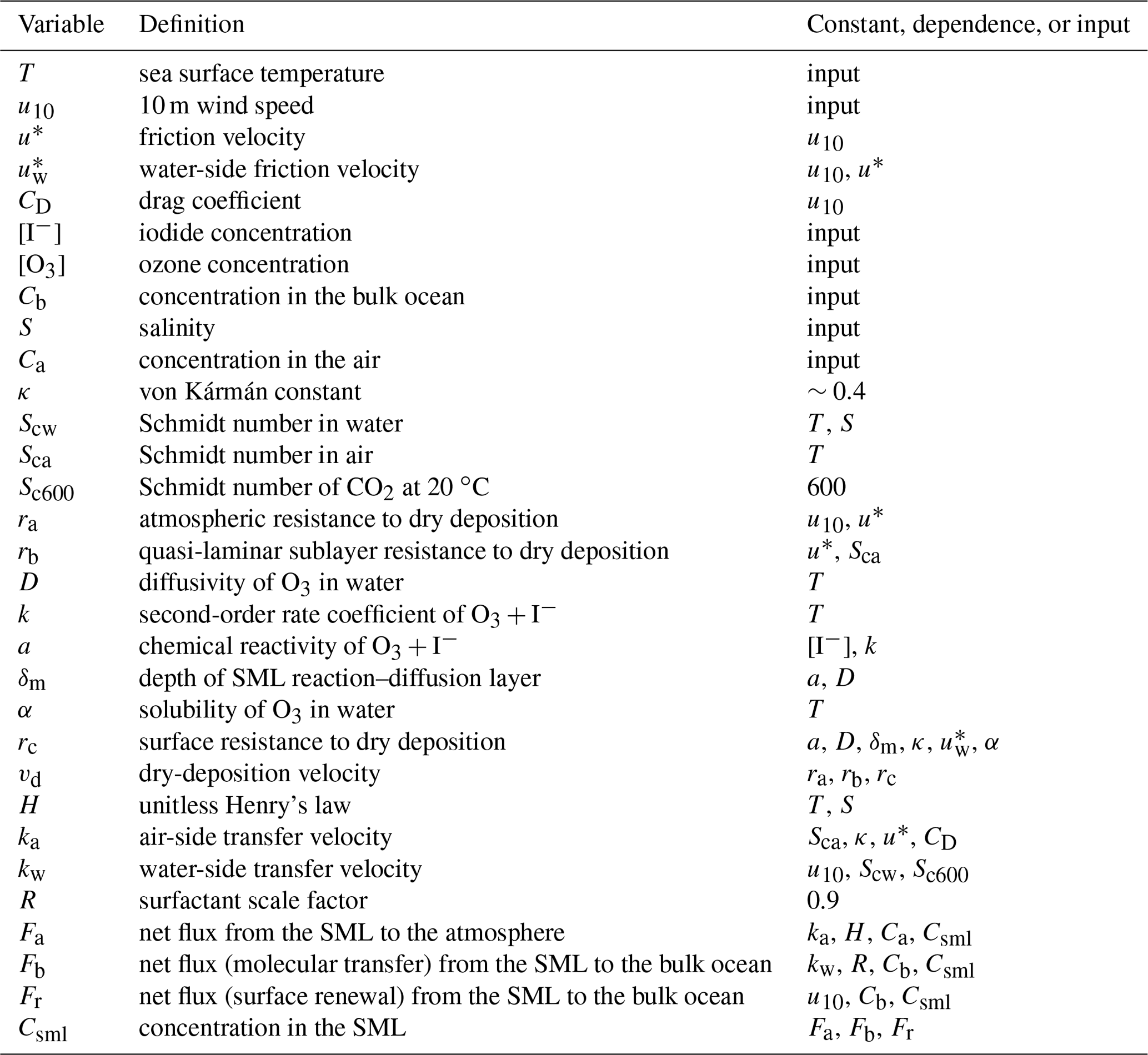
Figure 1 shows a simplified overview of the ocean–atmosphere exchange model described in this paper. Ozone deposition is based on the resistance-in-series scheme and is further described in Sect. 2.1. The SML is composed of many sublayers, defined by their physical, chemical, or biological properties (Soloviev and Lukas, 2014; Carpenter and Nightingale, 2015). This model considers only the top several micrometres of the SML, defined as the reaction–diffusion layer where the rate of chemical loss of O₃ dominates over turbulent transfer (Luhar et al., 2018). This length scale is dependent on the molecular diffusivity and chemical reactivity of O₃ and given by Eq. (8). The chemistry scheme employed is described in Sect. 2.2. Finally, the mixing of the SML with the atmosphere and the ocean is based on the method described by Cen-Lin and Tzung-May (2013), which is described in Sect. 2.3.1 and 2.3.2, respectively. Table 1 lists all the inputs, outputs, and variables used to calculate the flux of ozone into the SML and the emission of inorganic halogens from the SML.

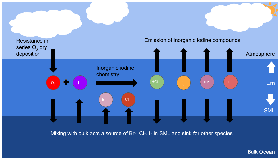
Figure 1 Overview diagram describing the physical arrangement of the ocean surface microlayer and the key chemical species included in the model. The black arrows represent the chemical fluxes and their net direction in this model.

Table 1 All input variables and calculated parameters along with their definitions and dependencies used by the model presented in this work for calculating the dry deposition of O₃ into the SML and fluxes of inorganic halogens to the atmosphere and bulk ocean from the SML.

The model was developed in Python using Cantera as the chemistry solver (Goodwin et al., 2022). The model presented here also uses functions from SciPy (Virtanen et al., 2020), Pandas (Development team, 2020), and NumPy (Harris et al., 2020). Calculations of the salinity- and temperature-dependent unitless Henry's law (H); Schmidt number in the air (S_ca); and water (S_cw), air-side (k_a), and water-side (k_w) transfer velocities are calculated using the recommended functions from Johnson (2010). The model runs presented here used a physical time step of $\mathrm{1}\times {\mathrm{10}}^{-\mathrm{4}}$ s and typically reach equilibrium within 4 s.

2.1 Coupled ozone dry deposition

Ozone dry-deposition velocity (v_d) is calculated using the resistance-in-series scheme based on Wesely and Hicks (1977), Eq. (1), this is then used to calculate the flux of ozone into the ocean surface microlayer. Air-side resistances that represent turbulent transport to the surface (r_a) and transport through the atmospheric quasi-laminar sub-layer, which is the air directly above the surface microlayer (r_b), are calculated using Eqs. (2) and (3), respectively (Chang et al., 2004):

$$\begin{array}{}\text{(1)}& {\displaystyle }& {\displaystyle }{v}_{\mathrm{d}}={\displaystyle \frac{\mathrm{1}}{r_{\mathrm{a}}+r_{\mathrm{b}}+r_{\mathrm{c}}}},\text{(2)}& {\displaystyle }& {\displaystyle }{r}_{\mathrm{a}}={\displaystyle \frac{u_{\mathrm{10}}}{u^{*\mathrm{2}}}},\text{(3)}& {\displaystyle }& {\displaystyle }{r}_{\mathrm{b}}={\displaystyle \frac{\mathrm{5}}{u^{*}}}{S}_{\mathrm{ca}}^{\mathrm{2}/\mathrm{3}},\end{array}$$

where u is the 10 m wind speed with units of m s⁻¹, u^* is the friction velocity with units of m s⁻¹, and S_ca is the Schmidt number of O₃ in air and is calculated using the method from Tsilingiris (2008) as recommended by Johnson (2010).

The surface resistance (r_c) captures the chemical and physical processes in the SML that control ozone loss. We employ the two-layer method of Luhar et al. (2018) to calculate r_c, which is shown in Eq. (4).

$$\begin{array}{}\text{(4)}& r_{\mathrm{c}}={\displaystyle \frac{\mathrm{1}}{\mathit{\alpha }\sqrt{aD}}}\left[{\displaystyle \frac{\mathrm{\Psi }{K}_{\mathrm{1}}\left({\mathit{\xi }}_{\mathit{\delta }}\right)\sinh \left(\mathit{\lambda }\right)+K_{\mathrm{0}}\left({\mathit{\xi }}_{\mathit{\delta }}\right)\cosh \left(\mathit{\lambda }\right)}{\mathrm{\Psi }{K}_{\mathrm{1}}\left({\mathit{\xi }}_{\mathit{\delta }}\right)\cosh \left(\mathit{\lambda }\right)+K_{\mathrm{0}}\left({\mathit{\xi }}_{\mathit{\delta }}\right)\sinh \left(\mathit{\lambda }\right)}}\right]\end{array}$$

The terms ξ_δ, Ψ, and λ are given in Eqs. (5), (6), and (7), respectively:

$$\begin{array}{}\text{(5)}& {\displaystyle }& {\displaystyle }{\mathit{\xi }}_{\mathit{\delta }}={\left[{\displaystyle \frac{\mathrm{4}a}{\mathit{\kappa }{u}_{\mathrm{w}}^{*}}}\left({\mathit{\delta }}_{\mathrm{m}}+{\displaystyle \frac{D}{\mathit{\kappa }{u}_{\mathrm{w}}^{*}}}\right)\right]}^{\frac{\mathrm{1}}{\mathrm{2}}},\text{(6)}& {\displaystyle }& {\displaystyle }\mathrm{\Psi }={\left[\mathrm{1}+\left({\displaystyle \frac{\mathit{\kappa }{u}_{\mathrm{w}}^{*}{\mathit{\delta }}_{\mathrm{m}}}{D}}\right)\right]}^{\frac{\mathrm{1}}{\mathrm{2}}},\text{(7)}& {\displaystyle }& {\displaystyle }\mathit{\lambda }={\mathit{\delta }}_{\mathrm{m}}\sqrt{{\displaystyle \frac{a}{D}}},\end{array}$$

where $u_{\mathrm{w}}^{*}$ (m s⁻¹) is the water-side friction velocity and δ_m is the thickness of the reaction–diffusion layer of the sea surface microlayer (m) calculated using Eq. (8) (Luhar et al., 2017). K₀ and K₁ are modified Bessel functions of the second kind with order 0 and 1, respectively, and κ is the von Kármán constant (≈0.4); a is the chemical reactivity of O₃ with I⁻ (defined in Eq. 9). It uses the second-order rate coefficient (k) from either Magi et al. (1997) or Brown et al. (2024) with units of M⁻¹ s⁻¹. The diffusivity O₃ in the SML (D, m² s⁻¹) is from Johnson and Davis (1996) and shown in Eq. (10). This calculation of D does not account for the impact of organics (particularly surfactants), which will impact the transfer of O₃ into the SML; this model is currently limited to inorganic chemistry, and the limitations of this are discussed further in Sect. 11. Here, α is the dimensionless solubility of O₃ from Morris (1988) shown in Eq. (11).

$$\begin{array}{}\text{(8)}& {\displaystyle }& {\displaystyle }{\mathit{\delta }}_{\mathrm{m}}=\sqrt{{\displaystyle \frac{D}{a}}}\text{(9)}& {\displaystyle }& {\displaystyle }a=k\left[{\mathrm{I}}^{-}\right]\text{(10)}& {\displaystyle }& {\displaystyle }D=\mathrm{1.1}\times {\mathrm{10}}^{-\mathrm{6}}\exp \left({\displaystyle \frac{-\mathrm{1896}}{T}}\right)\text{(11)}& {\displaystyle }& {\displaystyle }\mathit{\alpha }={\mathrm{10}}^{-\mathrm{0.25}-\mathrm{0.013}(T-\mathrm{273.16})}.\end{array}$$

The dry-deposition velocity (v_d) is coupled to the SML chemistry via the I⁻ concentration and is recalculated as the model advances in time towards equilibrium.

2.2 Chemistry

The aqueous inorganic halogen chemistry scheme used in this model is shown in Table 2. Here we employ an extended version of the iodine chemistry scheme used by Carpenter et al. (2013) and similar to that of Schneider et al. (2023) with the addition of further inter-halogen reactions involving bromine and chlorine species. A further difference between this chemistry scheme and that of Carpenter et al. (2021) is that we explicitly include the reaction step of O₃ + I⁻ producing IO⁻ (Reaction R1a) rather than HOI directly, alongside its subsequent conversion to HOI (Reaction R7). This has little impact on the total simulated inorganic iodine emissions as IO⁻ quickly reacts to form HOI at ocean pH, but it presents a more complete representation of the chemistry.

Magi et al. (1997)Brown et al. (2024)Lengyel et al. (1993)Lengyel et al. (1993)Lengyel et al. (1993)Paquette (1989)Sebők-Nagy and Körtvélyesi (2004)Paquette (1989)Bichsel and von Gunten (2000)Paquette (1989)Lengyel et al. (1993)Lengyel et al. (1993)De Barros Faria et al. (1993)Wang et al. (1989)De Barros Faria et al. (1993)Kumar et al. (1986)Schneider et al. (2023)Kumar et al. (1986)Kumar et al. (1986)Kumar et al. (1986)Nagy et al. (1988)Citri and Epstein (1988)Lengyel et al. (1996)Levanov et al. (2019)Haag and Hoigné (1983)Wang et al. (1994)Beckwith et al. (1996)Wang and Margerum (1994)Kumar and Margerum (1987)Wang et al. (1994)Beckwith et al. (1996)Wang and Margerum (1994)Michalowski et al. (2000)Michalowski et al. (2000)Michalowski et al. (2000)Wang et al. (1994)Wang et al. (1994)Wang et al. (1994)

Table 2 All reactions included in the chemistry scheme of this SML model with forward and reverse rate constants (where applicable) and accompanying references. Numbered reactions with a and b denote different rates explored in the sensitivity analysis conducted in this paper. The (1) is used to indicate $A=\mathrm{1.44}\times {\mathrm{10}}^{\mathrm{22}}$ M⁻¹ s⁻¹ and Ea=73.08 kJ mol⁻¹. The (2) is used to indicate $A=\mathrm{2.6}\times {\mathrm{10}}^{\mathrm{11}}$ M⁻¹ s⁻¹ and Ea=10.6 kJ mol⁻¹. The (3) is used to indicate the assumed reaction based on theoretical calculation.

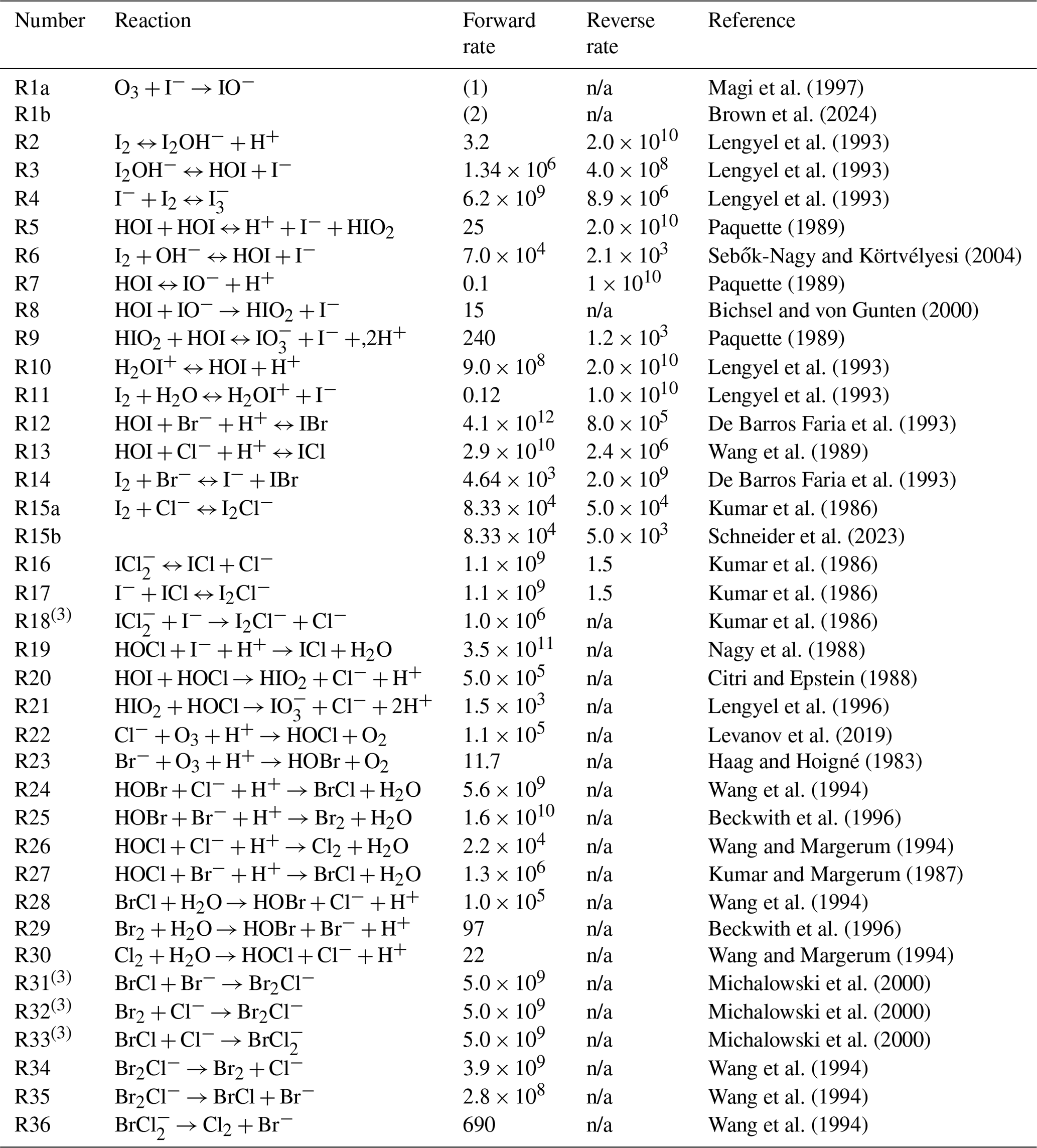
n/a: not applicable.

To explore the sensitivity of total iodine emissions to the rate coefficient of the O₃ + I⁻ reaction, two different forms of the temperature-dependent rate coefficient are used. The first of these (reaction R1a from Table 2) uses the rate published by Magi et al. (1997), which is also the rate used by Carpenter et al. (2013) in their model. The second rate (Reaction R1b from Table 2) is the more recent temperature-dependent rate from Brown et al. (2024), which has a much weaker temperature dependence than that of Magi et al. (1997). The different temperature dependencies of these two rates are shown in Fig. 2.

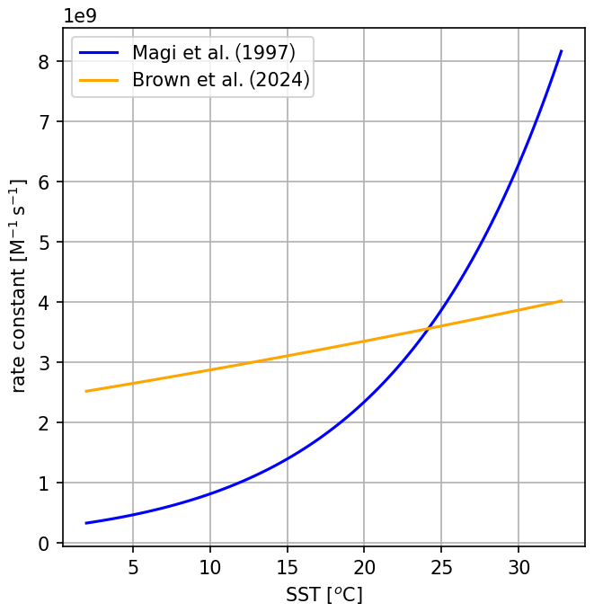
Figure 2 Comparison of the two published temperature-dependent rate coefficients from Magi et al. (1997) (blue) and Brown et al. (2024) (orange).

2.3 Mixing processes

2.3.1 Emissions of inorganic iodine

The net flux of a species from the SML into the atmosphere (F_a) is calculated from the concentration in the SML (C_sml) and the concentration in the atmosphere (C_a, Eq. 12). Atmospheric fluxes are calculated for HOI, I₂, IBr, ICl, HOCl, HOBr, Br₂, Cl₂, and BrCl. HOI and I₂ have the largest fluxes, with the other species emitted in negligible amounts due to their high solubility and relatively low concentrations in the SML.

$$\begin{array}{}\text{(12)}& F_{\mathrm{a}}=k_{\mathrm{a}}\left(H\cdot C_{\mathrm{sml}}-C_{\mathrm{a}}\right)\end{array}$$

k_a is calculated following the recommendation from Johnson (2010) using Eq. (13):

$$\begin{array}{}\text{(13)}& k_{\mathrm{a}}=+{\displaystyle \frac{u_{*}}{\mathrm{13.3}{S}_{\mathrm{ca}}^{\mathrm{0.5}}+C_{\mathrm{D}}^{-\mathrm{0.5}}-\mathrm{5}+\frac{\ln \left(S_{\mathrm{ca}}\right)}{\mathrm{2}\mathit{\kappa }}}},\end{array}$$

where u_* is the friction velocity (m s⁻¹) and C_D is the drag coefficient (m s⁻¹) from Smith (1980)

$$\begin{array}{}\text{(14)}& {\mathrm{10}}^{\mathrm{3}}{C}_{\mathrm{D}}=\mathrm{0.61}+\mathrm{0.063}{u}_{\mathrm{10}}.\end{array}$$

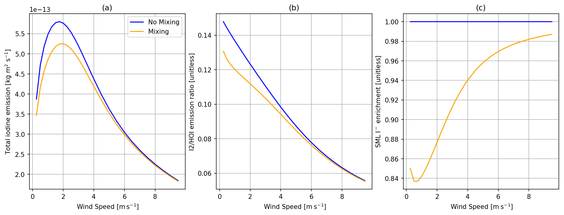
Figure 3 Comparisons of the SML model predictions with no mixing of I⁻ (100 nM in both the SML and bulk layers) (blue) and mixing of I⁻ from the bulk layer and varying in the SML (orange). (a) Total inorganic iodine emission (HOI + I₂ + IBr + ICl) vs. wind speed, (b) the ratio of I₂ $/$ HOI emission vs. wind speed, and (c) SML I⁻ enrichment (SML concentration/bulk concentration) vs. wind speed. All calculations are performed at 30 ppb of atmospheric O₃, 100 nM I⁻ concentration in bulk water, and 285 K sea surface temperature (SST).

2.3.2 Ocean mixing with SML

This model employs SML concentrations mixing with the bulk ocean concentration (C_b) on two timescales and follows the approach used by Cen-Lin and Tzung-May (2013). The first mixing process, molecular transfer, occurs on the order of 0.1–1 s and is given by Eq. (15).

$$\begin{array}{}\text{(15)}& F_{\mathrm{b}}=R{k}_{\mathrm{w}}\left(C_{\mathrm{b}}-C_{\mathrm{sml}}\right),\end{array}$$

where R accounts for the effects of surfactants suppressing the transport between the SML and bulk ocean. A value of 0.9 is used in this study to represent the open ocean (Goldman et al., 1988; Frew et al., 1990; Cen-Lin and Tzung-May, 2013). k_w is calculated using Eq. (16), which follows the recommendations of Johnson (2010) in using the Nightingale et al. (2000) approach. u₁₀ is the 10 m wind speed, S_cw is the Schmidt number of the gas in water, and S_c600 Schmidt number of CO₂ at 20 °C.

$$\begin{array}{}\text{(16)}& k_{\mathrm{w}}=\left(\mathrm{0.222}{u}_{\mathrm{10}}^{\mathrm{2}}+\mathrm{0.333}{u}_{\mathrm{10}}\right){\left({\displaystyle \frac{S_{\mathrm{cw}}}{S_{\mathrm{c}\mathrm{600}}}}\right)}^{\mathrm{0.5}}\end{array}$$

The second mixing process is surface renewal, representative of larger-scale eddy mixing, and is given by Eq. (17). It is a significantly slower process than the mixing described above and is typically on the order of minutes or longer but has been included for completeness. Surface renewal and the suppression of transfer velocity by surfactants (R) are new developments in this model compared to Carpenter et al. (2013).

$$\begin{array}{}\text{(17)}& F_{\mathrm{r}}=\left(\mathrm{3.42}\times {\mathrm{10}}^{-\mathrm{3}}{u}_{\mathrm{10}}+\mathrm{2.7}\times {\mathrm{10}}^{-\mathrm{3}}\right)\left(C_{\mathrm{b}}-C_{\mathrm{sml}}\right)\end{array}$$

Fluxes for mixing between the SML and bulk ocean are calculated for HOI, I₂, O₃, IBr, ICl, IO${}_{\mathrm{3}}^{-}$, HOBr, HOCl, Br₂, Cl₂, BrCl, I⁻, Br⁻, and Cl⁻. The mixing processes described here are only representative of passive diffusion and do not take into account any electrostatic effects. Solutions with ions have been found to have stronger electric fields at the air–water interface than within the bulk due to charge separation and this can contribute to an increased concentration of ions and enhanced reaction rates (Xiong et al., 2020; Hao et al., 2022). However, given that the fast turbulent-driven mixing of the SML with the bulk water and the chemical depletion of I⁻ within the SML occur on timescales of seconds or less under typical conditions, we consider additional effects that could impact the enhancement or depletion of I⁻ within the SML as likely being secondary. The control of I⁻ in the SML by the equilibrium of chemical and physical processes represents a significant difference between this work and that of Carpenter et al. (2013), where it was prescribed as a constant. The impact of this difference is explored in Sect. 3.

The concentration of I⁻ is set based on the conditions being studied by the model. Unless otherwise stated, the sensitivity studies presented here use a concentration of 100 nM. Br⁻ concentrations are set at 0.86 mM and Cl⁻ at 0.55 M to replicate typical ocean salinity. The oceanic concentration of IO${}_{\mathrm{3}}^{-}$ is set at 200 nM (Chance et al., 2020). All other species are assumed to have zero bulk oceanic concentrations. H⁺ and OH⁻ are not subject to mixing and are manually set at each time step to maintain a constant pH of 8.

3 Depletion of SML iodide

One difference between this and previous work is the model prediction of depletion of I⁻ in the SML at low wind speeds (Figs. 3 and 4) due to its reaction with O₃. This is a direct consequence of the slow replenishment of I⁻ in the SML from mixing with bulk water rather than being a fixed quantity as in previous models. Depletion of I⁻ has been previously detected experimentally in artificial seawater (Schneider et al., 2023). The effect of this depletion on total inorganic iodine emission and the composition of that emission is shown in Fig. 3. To a lesser extent, depletion of I⁻ is also greater at higher sea surface temperature (SST), as shown in Fig. 4; this is entirely driven by the temperature dependence of the O₃ + I⁻ reaction.

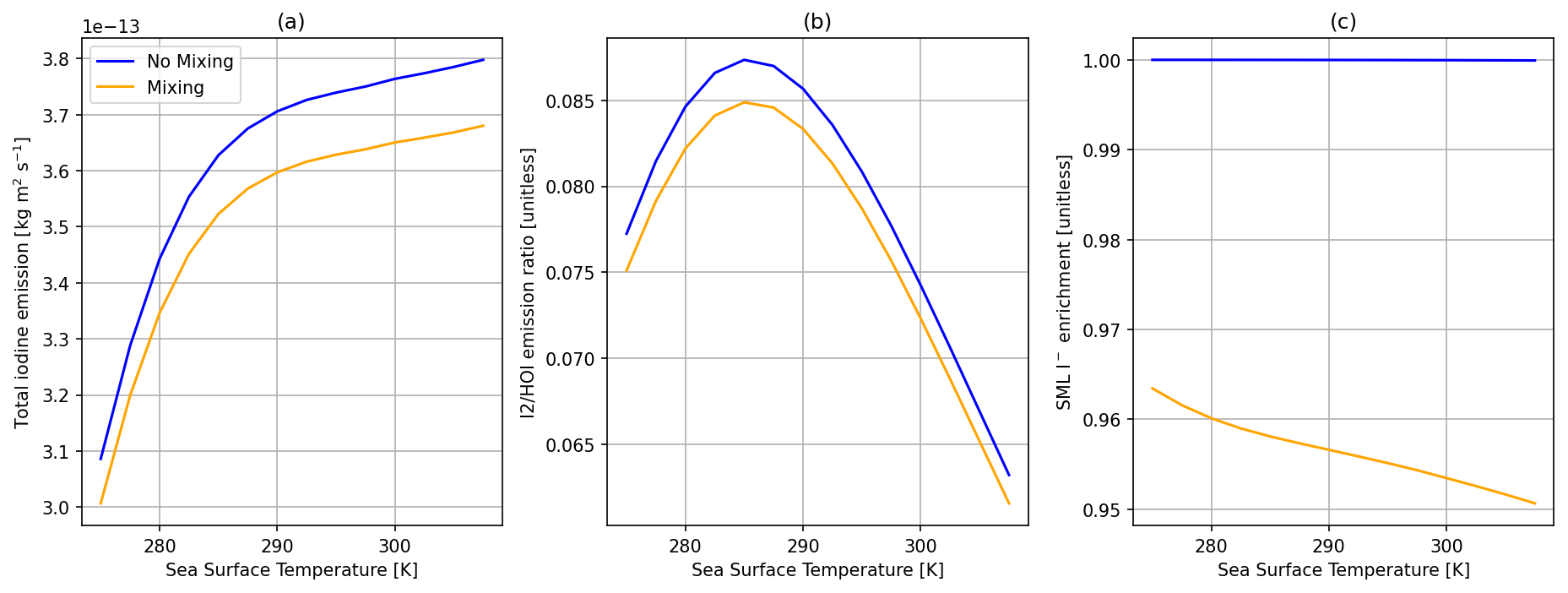
Figure 4 Comparisons of the SML model predictions with no mixing of I⁻ (100 nM in both the SML and bulk layers) (blue) and mixing of I⁻ from the bulk layer and varying concentration in the SML (orange). (a) Total inorganic iodine emission (HOI + I₂ + IBr + ICl) vs. SST. (b) The ratio of I₂ $/$ HOI emission vs. SST. (c) SML I⁻ enrichment (SML concentration/bulk concentration) vs. SST. All calculations are performed at 30 ppb of atmospheric O₃, 100 nM I⁻ concentration in bulk water, and 5 m s⁻¹ wind speed.

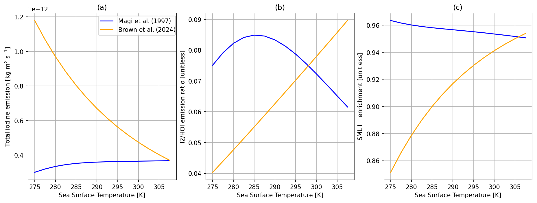
Figure 5 Comparisons of the SML model with the I⁻ + O₃ rate reported by Magi et al. (1997) (blue) and Brown et al. (2024) (orange). (a) Total inorganic iodine emission vs. SST. (b) The ratio of I₂ $/$ HOI emission vs. SST. (c) SML I⁻ enrichment (SML concentration/bulk concentration) vs. SST. All calculations are performed at 30 ppb of atmospheric O₃, 5 m s⁻¹ wind speed, and 100 nM I⁻ concentration in bulk water.

The depletion of I⁻ accounts for roughly an 11 % reduction in total inorganic iodine emissions at 2 m s⁻¹ wind speed, 285 K, 30 ppb O₃, and 100 nM of I⁻ in bulk water (Fig. 3). The reduction in SML I⁻ concentration also reduces O₃ dry-deposition velocity by 15 % under the same conditions.

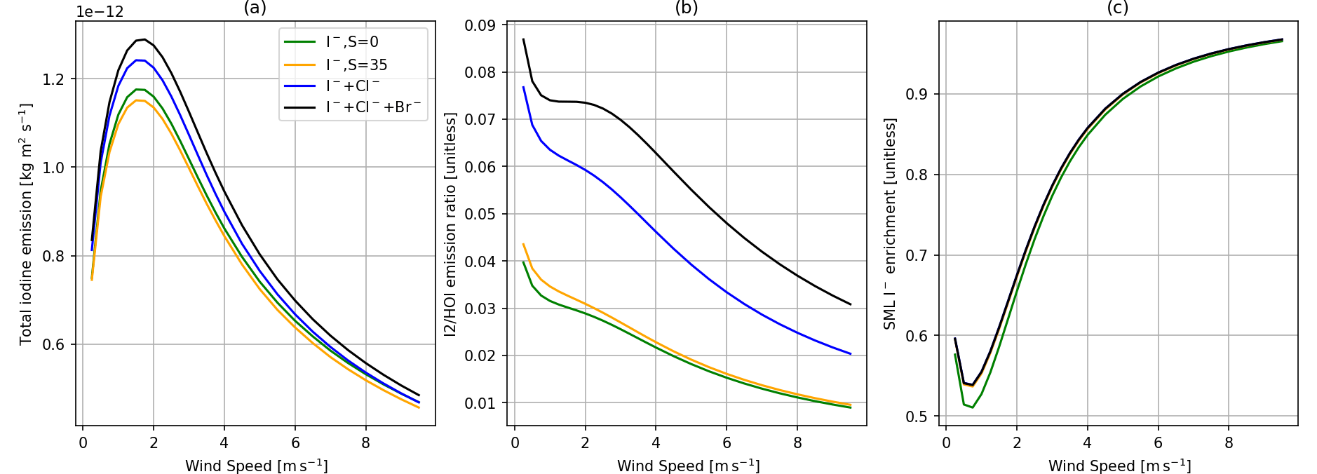
Figure 6 Comparisons of the SML model with only iodine chemistry (green), only iodine chemistry but with a salinity of 35 PSU (orange), iodine and chlorine chemistry (blue), and with the full chemistry scheme present (iodine, bromine, and chlorine chemistry, black). Panel (a) shows total inorganic iodine emission vs. wind speed, panel (b) shows the ratio of I₂ $/$ HOI emission vs. wind speed, and panel (c) shows SML I⁻ enrichment (SML concentration/bulk concentration) vs. wind speed. All calculations are performed at 30 ppb of atmospheric O₃, 285 K SST, and 100 nM I⁻ concentration in bulk water.

4 Sensitivity to the temperature dependence of the I⁻ + O₃ reaction

Here we compare two temperature-dependent rate constants for the I⁻ + O₃ reaction. The first of these is that of Magi et al. (1997), which has been used in the previous model of Carpenter et al. (2013). We compare this to the more recent rate from Brown et al. (2024), which was derived from experiments conducted at I⁻ concentrations of ∼100–10 000 nM. The difference in the temperature dependence of total inorganic iodine emission is shown in Fig. 5. The newer rate constant results in substantially higher total inorganic iodine emissions at low SST. At 285 K, total inorganic iodine emissions increase by ∼130 % when using the rate coefficient from Brown et al. (2024) compared to Magi et al. (1997) (Fig. 5a), while O₃ dry-deposition velocity increases by 36 %. Both increases are offset by I⁻ enrichment decreasing from ∼96 % to ∼90 % at the same temperature (Fig. 5c). Increased depletion of I⁻ in the SML also results in the production pathways of I₂ from HOI becoming less competitive, resulting in the amount of I₂ emission relative to HOI decreasing (Fig. 5b). At higher temperatures (above ∼25 °C, Fig. 2), the Brown et al. (2024) rate is slower than that of Magi et al. (1997), resulting in decreased HOI production; however, this is somewhat offset by the sensitivity of the model to the reaction–diffusion length, which is dependent on this rate and is explored in Sect. 6. All subsequent experiments using the box model use the Brown et al. (2024) rate due to it better reflecting the O₃ + I⁻ reaction under oceanic conditions.

5 I₂ emission salinity sensitivity

The experimental work of MacDonald et al. (2014) found a strong increase in I₂ emission at higher salinity, which was replicated in their accompanying model results. We also predict a positive salinity dependence on I₂ emissions in our base model (Fig. 6). The increase in I₂ emissions is partly from the additional chemical pathway to produce I₂ via ICl as concluded by MacDonald et al. (2014) (Reactions R13, R15 and R17 in Table 2). Additionally, the changes in solubility (due to salinity due to the salinity dependence of H and S_cw, salting out effect) increase the total iodine emissions, as shown by the difference between the green and yellow lines in Fig. 6, where the chloride concentration was set to achieve a salinity of 35 PSU but the chlorine chemistry was removed from the chemical mechanism. The increase in total iodine emissions from the increase in I₂ emission has a negligible impact on HOI emissions, as HOI is in excess in the SML (Carpenter et al., 2013).

The largest increase in I₂ emission with the addition of salinity is observed in low-turbulence conditions (low wind speed, Fig. 6b); here the effects on solubility have a larger effect than the additional chemical pathway to I₂ production provided by Cl⁻. Under the conditions used in this study, I₂ emissions are increased by ∼150 % with the addition of Cl⁻. However, this is less than the 250 % increase observed by MacDonald et al. (2014). Differences between experimental results and this model are discussed further in Sect. 8. Figure 6 shows that, similar to chloride, increasing bromide increases total I₂ production. This increase is the result of the additional pathway via IBr to produce I₂ (Reactions R12 and R14 in Table 2).

In contrast to these results, more recent work from Tinel et al. (2020) and Schneider et al. (2023) did not find an increase in I₂ emissions from increasing Cl⁻. I₂ emissions were instead suppressed in saline samples compared to purely iodide solutions. Schneider et al. (2023) found that their results could be replicated by shifting the equilibrium for Reaction R15a in Table 2 to favour I₂Cl⁻ over I₂ (Reaction R15b in Table 2). The result of implementing that change to the equilibrium in this model is shown in Fig. 7. The rate of I₂ production through the additional chemical pathway provided by ICl is reduced, and iodine emissions decrease by up to 5 %. Depletion of I⁻ is unaffected.

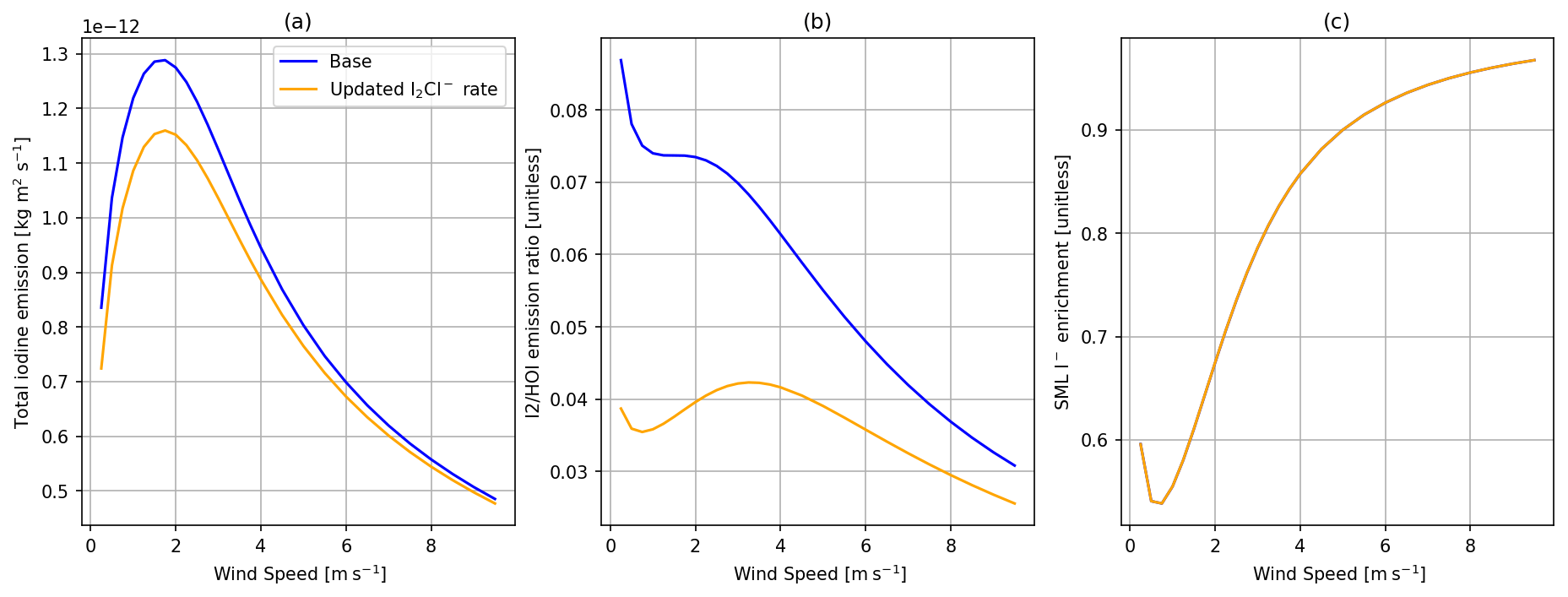
Figure 7 Comparisons of the SML model with I⁻ + O₃ rate using the standard chemistry scheme (blue) and the updated equilibrium from Schneider et al. (2023) (orange). Panel (a) shows total inorganic iodine emission vs. wind speed, panel (b) shows the ratio of I₂ $/$ HOI emission vs. wind speed, and panel (c) shows SML I⁻ enrichment (SML concentration/bulk concentration) vs. wind speed, with all calculations using 30 ppbv of atmospheric O₃, 285 K SST, and 100 nM I⁻.

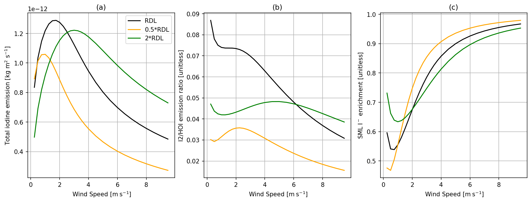
Figure 8 Comparisons of the SML model with the depth of the model being half (orange) and twice (green) the reaction–diffusive length (RDL) and the base model using a single reaction–diffusion length (black). Panel (a) shows total inorganic iodine emission vs. wind speed, panel (b) shows the ratio of I₂ $/$ HOI emission vs. wind speed, and panel (c) shows SML I⁻ enrichment (SML concentration/bulk concentration) vs. wind speed, with all calculations using 30 ppbv of atmospheric O₃, 285 K wind speed, and 100 nM I⁻.

6 Inorganic iodine emission sensitivity to reaction–diffusion layer depth

Here we explore the sensitivity of predicted iodine emission fluxes to the depth of the reaction–diffusion layer (δ_m). The values of δ_m calculated are typically between 2.2–2.9 µm for the conditions shown in Figs. 8 and 9 (using Eq. 8 and the Brown et al., 2024, rate constant). δ_m is directly dependent on SML temperature via O₃ diffusivity D and the chemical reactivity a, with a also giving δ_m a direct dependence on [I⁻]. There is an indirect dependence between δ_m and wind speed due to the depletion of iodide in the SML that increases in low-turbulence conditions. Under conditions with higher turbulence (>3 m s⁻¹), larger δ_m values increase total inorganic iodine emissions. However, under less well-mixed conditions, the coupling of mixing and the availability of I⁻ in the SML creates a more complex relationship between total inorganic iodine emission and δ_m. Further improvements to model predictions of total inorganic iodine emissions are therefore dependent on our understanding of the reaction–diffusion length and uncertainties in both D and the rate of O₃ + I⁻ (Reaction R1).

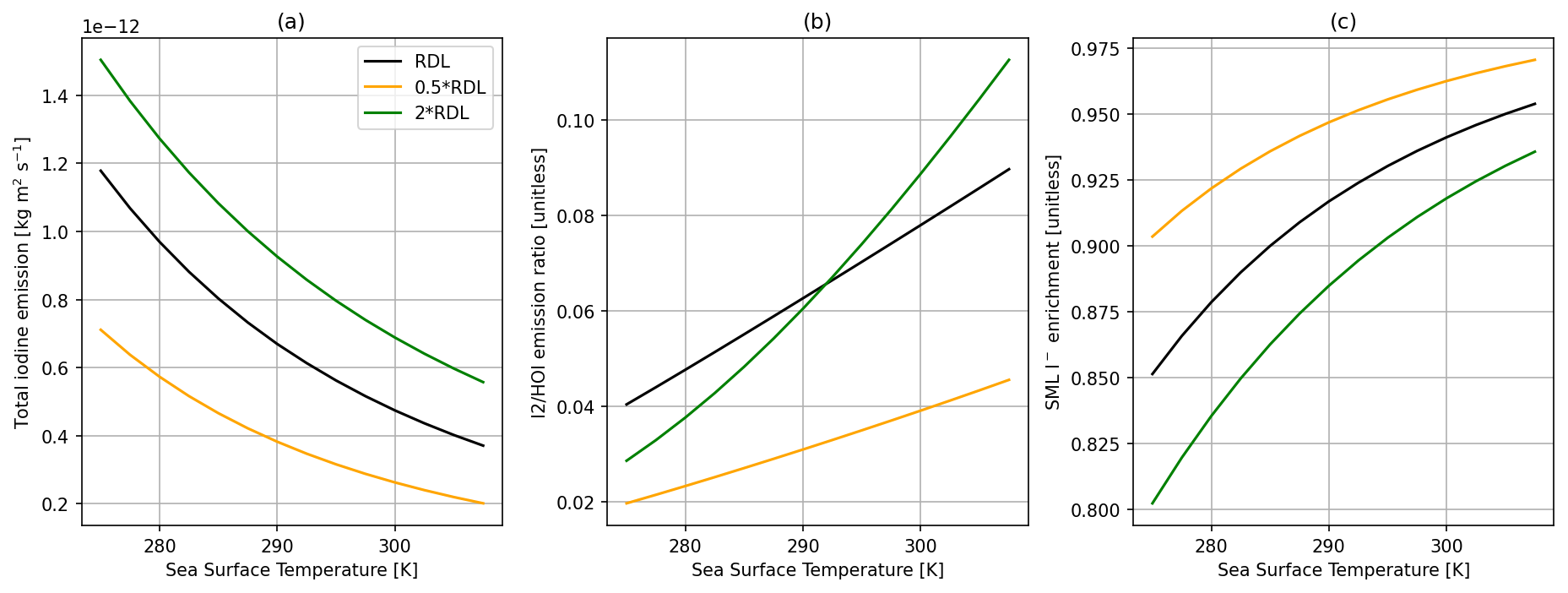
Figure 9 Comparisons of the SML model with the depth of the model being half (orange) and twice (green) the reaction–diffusive length (RDL) and the base model using a single reaction–diffusion length (black). Panel (a) shows total inorganic iodine emission vs. SST, panel (b) shows the ratio of I₂ $/$ HOI emission vs. SST, and panel (c) shows SML I⁻ enrichment (SML concentration/bulk concentration) vs. SST, with all calculations using 30 ppbv of atmospheric O₃, 5 m s⁻¹ wind speed, and 100 nM I⁻.

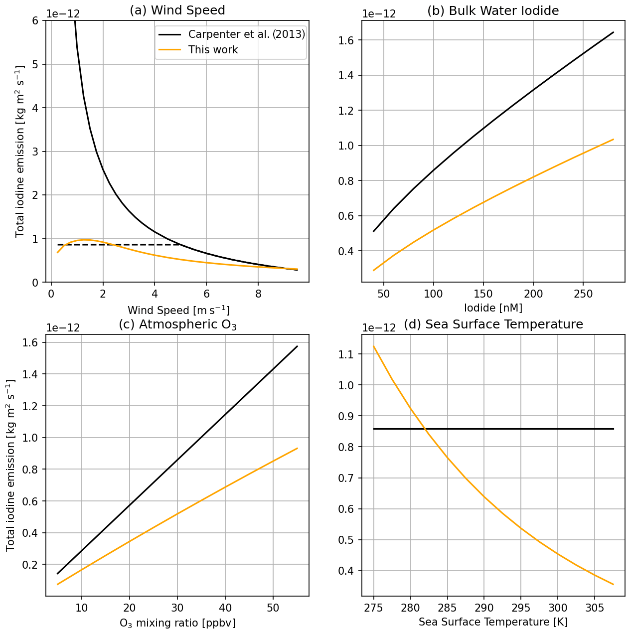
Figure 10 Comparison between total iodine emissions from this work and the model as implemented by Carpenter et al. (2013) across a range of wind speeds (a) (both with (dashed black line) and without (solid black line) a minimum wind speed of 5.5 m ⁻¹), bulk water iodide concentrations (b), atmospheric O₃ mixing ratios (c), and sea surface temperatures (d).

7 Comparisons to existing model

Figure 10 compares the total iodine emissions predicted in this work to that of Carpenter et al. (2013) across wind speed, iodide, ozone, and temperature ranges. The new model uses the O₃ + I⁻ rate from Brown et al. (2024) and the updated equilibrium of Reaction R15b from Schneider et al. (2023). Temperature dependence was not included in the Carpenter et al. (2013) equations. Two versions of the Carpenter et al. (2013) model are used in the wind speed comparison. The first is the equations as presented (solid black line), while the second has a minimum wind speed of 5.5 m s⁻¹ applied (dashed black line, as used in the global modelling study of Sherwen et al. (2016)). For total iodine emission at the highest wind speeds, the new model tends towards the old model. This is due to the efficient mixing at these higher wind speeds resulting in negligible I⁻ depletion in the SML, and it thus more closely resembles the old model, which included a constant I⁻ concentration in the SML. As wind speed decreases, the two models diverge in their prediction of total iodine emission, with the new model predicting less emission flux than the capped and uncapped (Carpenter et al., 2013) model. This decrease is most notable at very low wind speeds where the new model tends towards no iodine emission as wind speed tends towards zero, rather than the Carpenter et al. (2013) model where total iodine emissions exponentially increase as wind speed tends to zero.

Carpenter et al. (2013) found a simple multiplicative and approximately linear relationship between O₃ concentration and total iodine emission. The slightly dampened relationship between O₃ and total iodine emission in this model is likely because higher O₃ concentration causes a greater depleting effect on SML I⁻ concentration, reducing total iodine emission. The new model predicts a similar trend of I⁻ dependence of total iodine emission to Carpenter et al. (2013). Additionally, the new model predicts that I₂ contributes a larger percentage of total iodine emissions, despite the change made to the chemistry scheme to reflect lower I₂ emissions under oceanic salinity. This difference is likely due to a reduced HOI emission flux from the SML, resulting in more of the aqueous HOI remaining in the SML, which can subsequently produce more I₂.

8 Comparisons to experimental data

Table 3 compares published experimental results for I₂ fluxes to predictions from this model under conditions that match those used in the various experimental studies. One limitation in this comparison is replicating the water-side turbulence due to stirring (or not) of the aqueous solution and from the gas flow over the solution. Experimental setups which do not stir the solution have very different dynamics to the ocean surface, which this model has been designed to replicate. Additionally, some experimental results use O₃ and I⁻ concentrations significantly higher than typical environmental conditions due to measurement instrument sensitivity (Table 3). The model significantly underestimates experimental results where the solutions were not stirred, possibly due to a high depletion of surface iodide under such conditions, which reduces the potential for gaseous iodine emissions (Schneider et al., 2023). For stirred experiments, however, the model predicts a similar range of I₂ emissions as the experiments.

Carpenter et al. (2013)MacDonald et al. (2014)Tinel et al. (2020)Tinel et al. (2020)Schneider et al. (2023)

Table 3 Comparison of I₂ emissions from published experimental studies with the SML model of this study run using the experiment parameters. Ranges of I₂ emissions represent the range of both measured and calculated flux from the range of experimental inputs used. Model results were obtained with R=1 as no organics are present in these experimental results.

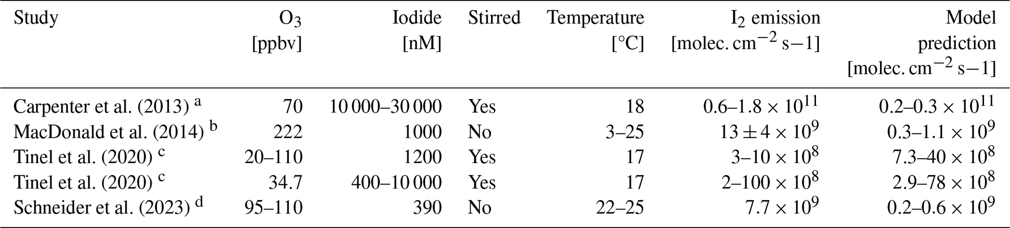
^a The pH 8 seawater spiked with iodide. ^b The pH 8 buffered solution with 0.5 M chloride and $\mathrm{1}\times {\mathrm{10}}^{-\mathrm{6}}$ M iodide. ^c Artificial seawater containing iodide, bromide, and chloride that has been buffered to pH 8. ^d Iodide only with a buffered pH 8 value.

9 Parameterized equation for HOI and I₂ emission flux

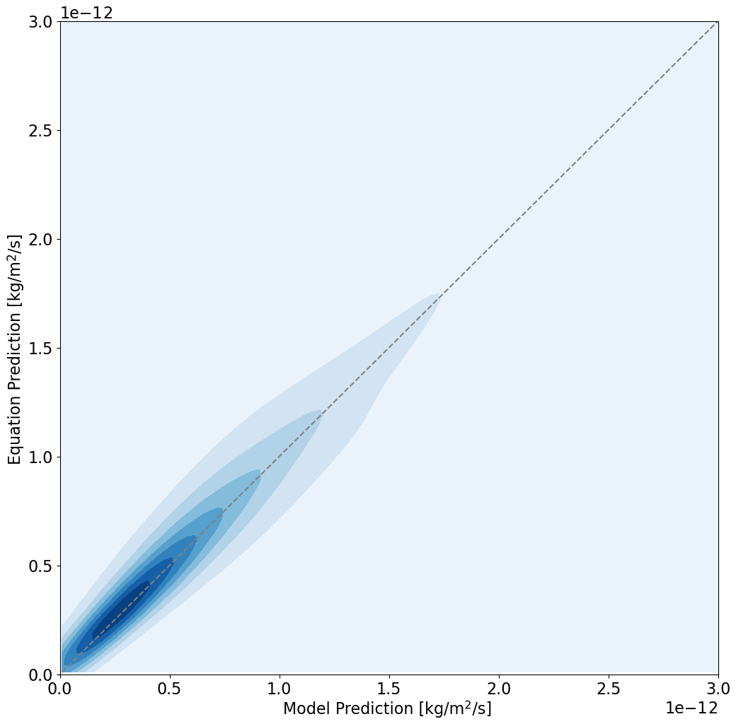
Here we present two mathematical functions to predict HOI (Eq. 18) and I₂ (Eq. 19) emission fluxes based on [O₃], bulk [I⁻], wind speed, and SST. A non-linear least-squares fit was used on 5000 unique combinations of model inputs covering environmentally comparable ranges of each variable (5–60 ppb of O₃, 0.1–11.1 m s⁻¹ wind speed, 20–240 nM bulk [I⁻], and 274–300 K SST). All other parameters are kept constant in the sensitivity analysis. The model sensitivity studies are run using the O₃ + I⁻ rate from Brown et al. (2024) and the updated equilibrium of Reaction R15b from Schneider et al. (2023). These equations have a high correlation with the results from the SML box model, i.e. R²=0.92 for HOI and R²=0.92 for I₂, and no strong bias in terms of overestimating or underestimating the model results (Fig. 11).

$$\begin{array}{}\text{(18)}& {\displaystyle }\begin{array}{rl}\mathrm{HOI}=& \mathrm{6.9}\times {\mathrm{10}}^{-\mathrm{11}}\left({\displaystyle \frac{u+\mathrm{6.2}}{\mathrm{12}}}\right)e^{-\mathrm{0.034}T-{\left(\frac{u+\mathrm{6.2}}{\mathrm{12}}\right)}^{\mathrm{2}}}\\ & {\left[{\mathrm{O}}_{\mathrm{3}}\right]}_{\mathrm{g}}^{\mathrm{0.92}}{\left[{\mathrm{I}}^{-}\right]}^{\mathrm{0.64}}\end{array}\text{(19)}& {\displaystyle }\begin{array}{rl}{I}_{\mathrm{2}}=& \mathrm{4.2}\times {\mathrm{10}}^{-\mathrm{19}}\left({\displaystyle \frac{u+\mathrm{3.1}}{\mathrm{7.2}}}\right)e^{\mathrm{0.011}T-{\left(\frac{u+\mathrm{3.1}}{\mathrm{7.2}}\right)}^{\mathrm{2}}}\\ & {\left[{\mathrm{O}}_{\mathrm{3}}\right]}_{\mathrm{g}}^{\mathrm{0.73}}{\left[{\mathrm{I}}^{-}\right]}^{\mathrm{1.5}}\end{array}\end{array}$$

Here HOI and I₂ emission are given in kg m⁻² s⁻¹, T is the sea surface temperature (K), u is the 10 m wind speed (m s⁻¹), [I⁻] is the bulk water iodide concentration (nM), and [O₃]_g is the atmospheric ozone mixing ratio (ppb).

Figure 11 Correlation between modelled total inorganic iodine emission and the sum of HOI + I₂ predicted using Eqs. (18) and (19).

The most notable difference between the parameterized equations presented here and those from Carpenter et al. (2013) is the inclusion of T as a parameter. Carpenter et al. (2013) found a linear relationship between both HOI and I₂ emissions and atmospheric O₃. This relationship with O₃ is reduced for HOI, which can be attributed to the impact of I⁻ depletion in the SML being increased at higher O₃ concentrations, reducing the rate at which the O₃ + I⁻ reaction can occur. The effect of O₃ concentration on I⁻ depletion is further enhanced for I₂ production (and hence a further reduction in the I₂ dependence on O₃ concentration) as the subsequent chemical pathways to convert HOI to I₂ also depend on the availability of I⁻ in the SML. I⁻ depletion can also explain the increase in dependence of HOI emission on SML [I⁻] (from a power of 0.5 to 0.63) and I₂ (from a power of 1.3 to 1.5) due to a relative increase in the availability of I⁻ in the SML at higher bulk water concentrations.

10 Implementing the new iodine emission equations in GEOS-Chem Classic

We use the GEOS-Chem classic model (Bey et al., 2001) version 14.1.1 (GCC14.1.1, 2023) for global modelling of inorganic iodine emissions and their impact on tropospheric composition. GEOS-Chem Classic is a chemical transport model with a HO_x–NO_x–VOC–O₃–halogen–aerosol tropospheric chemistry scheme. The current version of the halogen chemistry scheme is described by Wang et al. (2021), with organic iodine emissions based on Ordóñez et al. (2012) and inorganic iodine emissions based on Carpenter et al. (2013) (as implemented by Sherwen et al., 2016). The current inorganic iodine emissions in GEOS-Chem use surface oceanic iodide concentrations based on MacDonald et al. (2014), which under-predicts concentrations compared to observations (Sherwen et al., 2019) and differs from the iodide field used in calculating O₃ dry deposition, which uses Sherwen et al. (2019) (Pound et al., 2020). Here, we implement the equations for inorganic iodine emission presented in Sect. 8 and compare the impact of changing the iodide used from MacDonald et al. (2014) to the up-to-date and machine-learning-derived iodide climatology from Sherwen et al. (2019) for both inorganic iodine emissions, providing symmetry with the current use of this iodide climatology in O₃ dry deposition.

A global spatial resolution of 4°×5° on the standard vertical grid (72 vertical levels) is used, running with chemistry in both the troposphere and stratosphere. Meteorological data are from MERRA-2 (Gelaro et al., 2017). Three model runs that were identical in configuration were conducted, with the only difference being their inorganic iodine emissions. The first uses the default inorganic iodine emissions based on the equations from Carpenter et al. (2013) driven by MacDonald et al. (2014) oceanic I⁻. The second uses the new iodine emission equations presented in this work (Eqs. 18 and 19) driven by MacDonald et al. (2014) oceanic I⁻. The third uses the new iodine emission equations driven by Sherwen et al. (2019) oceanic I⁻. All other emission and time step configurations were left at their recommended settings. Model simulations were conducted from 1 July 2019 to 1 July 2021, with the first year of the simulation considered a “spin-up” to allow the model to reach equilibrium. Although the 2020–2021 period is within a La Niña event, a change in temperature of 1 K changes total inorganic iodine emissions by ∼3 % (Fig. 10). As such, temperature variations due to El Niño–Southern Oscillation (ENSO) are likely to result in changes in the inorganic iodine concentrations of less than 10 % locally and likely even less globally.

The new iodine emission equations decrease the total global inorganic iodine emissions from 2.84 to 2.78 Tg yr⁻¹, a decrease of 2 %. Additionally, there is a slight increase in the ratio of I₂ emissions compared to HOI, with I₂ now accounting for 5.9 % (previously 5.7 %); however, this difference would not change the impact of iodine on the troposphere as both HOI and I₂ rapidly photolyse. Whilst this is a relatively small global total change, there is a significant re-distribution of total iodine emissions, with emissions from equatorial waters decreasing and high-latitude emissions increasing, as shown in Fig. 12a. The changes in global emission distribution are largely driven by the change from the Magi et al. (1997) to the Brown et al. (2024) rate constant, with large increases in high-latitude waters also being the result of the base model predicting near-zero emissions in cold waters with low [I⁻]. Combining the new iodine emission equations with the Sherwen et al. (2019) (Fig. 12b) iodide climatology results in an additional factor of ∼4 increase in total inorganic iodine emission from high-latitude waters, decreasing to ∼1.5 outside of these regions. This iodide climatology increases the total global inorganic iodine emissions to 4.5 Tg yr⁻¹ (+49 %). Due to the substantially improved comparison with observations, the iodide climatology from Sherwen et al. (2019) will be used in the following analysis.

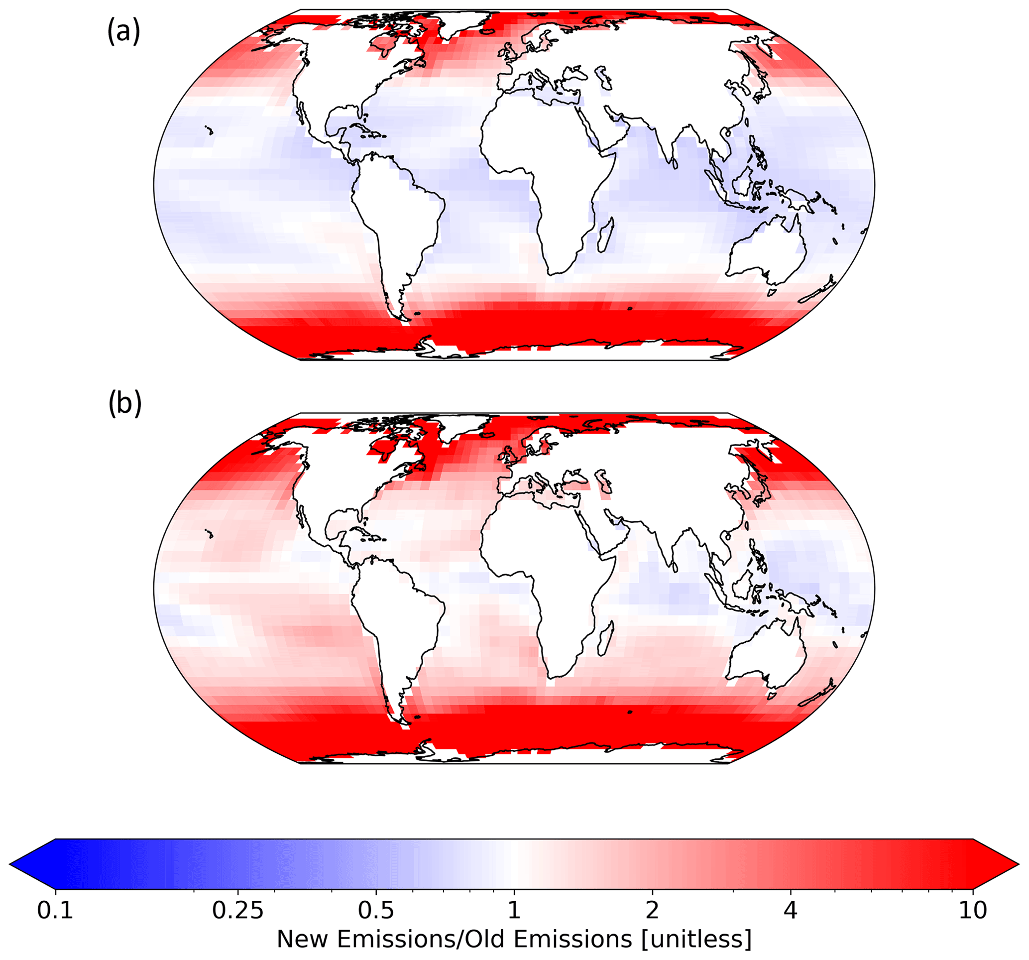
Figure 12 (a) Fractional change in the annual mean total inorganic iodine emissions from Carpenter et al. (2013) equations and MacDonald et al. (2014) (base) I⁻ to the new HOI and I₂ emission equations (Eqs. 18 and 19) and MacDonald et al. (2014). Panel (b) shows the change from base to the new HOI and I₂ emission equations and Sherwen et al. (2019) I⁻. The new version of inorganic iodine emission equations combined with Sherwen et al. (2019) sea surface iodide predicts higher emissions at higher latitudes and a decrease in emissions from warmer tropical waters.

The change in the distribution of inorganic iodine emissions substantially increases high-latitude IO (and IO_x) concentrations, with percentage changes of >1000 %, as the base case model predicts very low or no IO concentration in these regions (Fig. 13). Equatorial IO has small regional increases and some decreases, mirroring the negligible increases and localized decreases in inorganic iodine emissions from warm waters. However, despite large regional changes, the change in area-weighted mean vertical iodine speciation is minimal, with large percentage changes reflecting small absolute increases. Figure 14 compares published observations of average daytime surface IO mixing ratios to the model predictions from the corresponding day of the year during the simulated period. This comparison only considers open-ocean observations, whereas coastal observations of IO have large influences from macro-algae emissions (Saiz-Lopez and Plane, 2004) that are not included in this model. The change in iodine emissions has little effect on the average model root-mean-square error in atmospheric IO, increasing it from 0.48 to 0.62 ppt (0.43 to 0.58 ppt excluding polar observations), with a change in the relative mean bias from −0.43 to 0.43 ppt (−0.07 to 0.55 ppt excluding polar observations), suggesting that there are still uncertainties in other aspects of our understanding of the iodine system, such as the formation of HIO₃ (He et al., 2021; Huang et al., 2022) and the photolysis scheme currently used for higher-iodine oxides (Sherwen et al., 2016). Work to further understand the atmospheric chemistry of iodine is still required if we are to have confidence in the predictions of our models. Wang et al. (2021) found less disagreement between their model and observation comparisons; however, that study included sea salt debromination, which has a large impact on tropospheric O₃ and is by default deactivated in version 14.1.1 of GEOS-Chem. The increase in high-latitude oceanic emissions of HOI and I₂ reduces the model error at the two Antarctic locations (Bharati and Maitri bases) and the MOSAiC Arctic observations included in Fig. 14. However, the model still significantly underestimates IO levels in the Antarctic region. Atmospheric iodine observations made in the Antarctic region have been shown to have a source from sea ice (Saiz-Lopez et al., 2007; Atkinson et al., 2012) and a direct source of atmospheric IO from the snowpack (Frieß et al., 2010); these processes are not currently represented in the model.

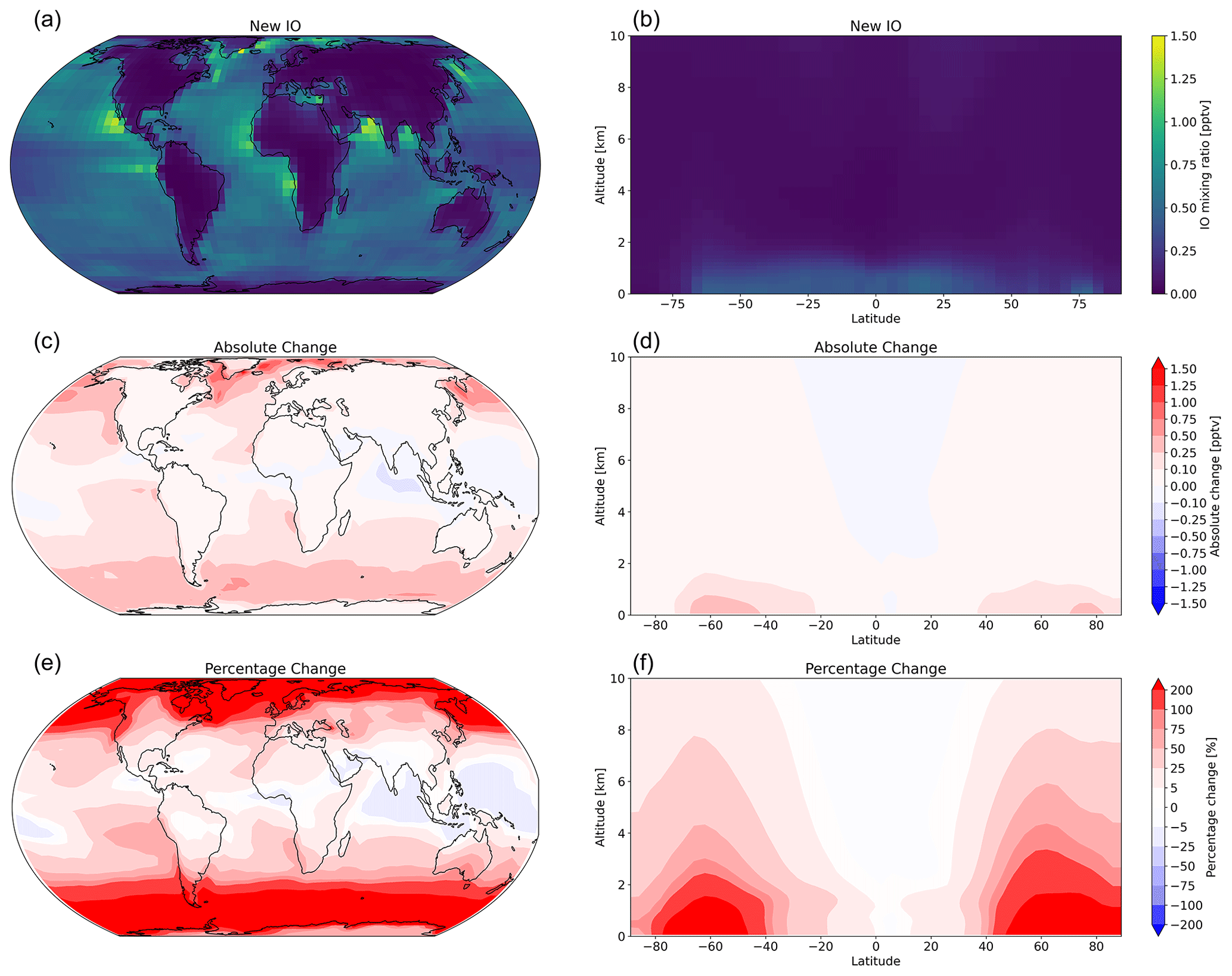
Figure 13 Annual mean mixing ratio of IO (a, b) using new inorganic iodine emissions and absolute change (c, d) and percentage change (e, f) in the annual mean atmospheric IO from implementing the new inorganic iodine emissions relative to the “base” model case, which used oceanic iodine emissions from Carpenter et al. (2013) and iodide from MacDonald et al. (2014).

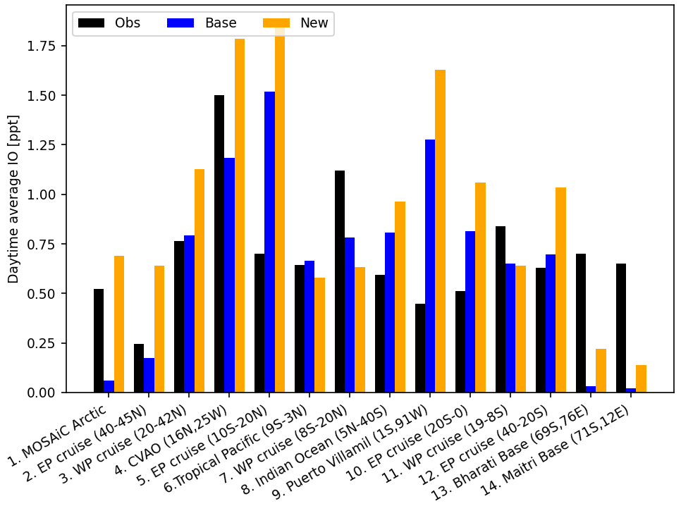
Figure 14 Daytime surface average IO mixing ratio from coastal sites and ocean cruises with observations (black) from reporting periods in different years. Model values are monthly mean daytime surface values taken from the same reporting month and location but from the years 2020/2021, where the base data set (blue) uses HOI and I₂ emissions from Carpenter et al. (2013) driven by MacDonald et al. (2014) iodide and the new data set (orange) uses the HOI and I₂ emissions presented in this work driven by Sherwen et al. (2019) iodide. References are as follows: (1) Mahajan (2022), (2, 5, 10, 12) Mahajan et al. (2012), (3, 7, 11) Großmann et al. (2013), (4) Mahajan et al. (2010), (6) Takashima et al. (2022), (8) Mahajan et al. (2019a, b), (9) Gómez Martín et al. (2013), (13, 14) Mahajan et al. (2021).

Despite the large increase in total inorganic iodine emissions, there is only a 1.5 % decrease in the tropospheric O₃ burden (from 330 to 325 Tg). As with IO, there are larger regional changes in both surface and zonal O₃, as shown in Fig. 15. Tropospheric O₃ at higher latitudes is decreased with the largest absolute and percentage changes above the Southern Ocean, while O₃ above the equatorial Indian Ocean and western central Pacific Ocean increases.

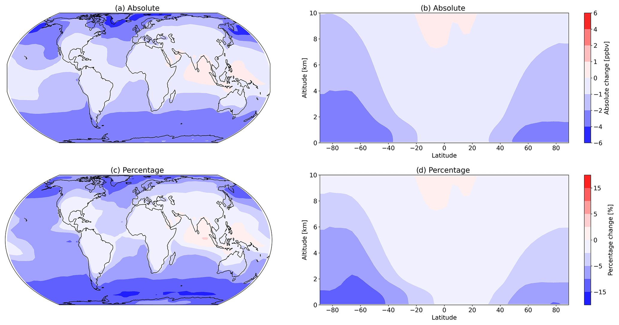
Figure 15 Absolute and percentage change in surface O₃ (a, c) and absolute and percentage change in zonal O₃ (b, d) due to changing the Carpenter et al. (2013) inorganic iodine emissions from the ocean to the equations presented in this work. The largest changes occur in the surface levels of the model, with the largest relative decrease in surface O₃ occurring over the Southern Ocean and the largest relative increase occurring over the Indian Ocean.

Figure 16 shows the impact of the change in iodine emissions on surface ozone predictions. For this, we compare the model to a selection of surface ozone measurements from several World Meteorological Organization (WMO) Global Atmosphere Watch sites around the world (GAW; http://www.wmo.int/pages/prog/arep/gaw/gaw_home_en.html, last access: October 2023, accessed through EBAS http://ebas.nilu.no/, last access: October 2023; the database infrastructure is operated by the Norwegian Institute for Air Research).

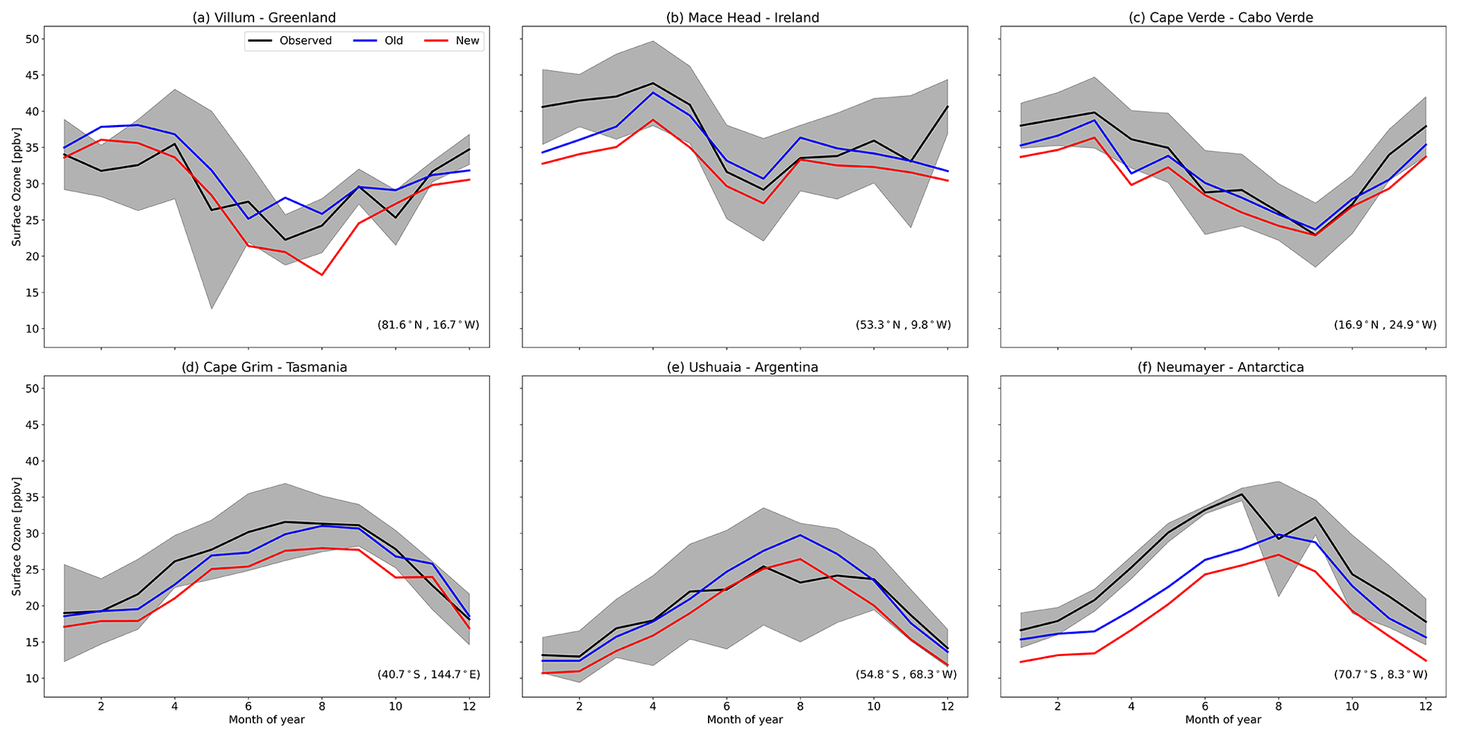
Figure 16 Predictions and observations of monthly average surface ozone mixing ratio from the model using the old iodine emissions (old) and the model using Eqs. (18) and (19) (new) for six GAW stations (with the latitude and longitude for each station at the bottom right), with the shaded region representing the 25th to 75th percentiles. Observational data are from 2014.

At the northern high latitudes, we compare to O₃ observations made in Greenland (Fig. 16a). The model disagreement at this site, measured using the root-mean-square error (RMSE), increases from 3.7 to 3.8 ppb (2.7 %); however, the model remains unable to replicate springtime O₃ depletion events that occur in the high latitudes.

Mace Head, Ireland (Fig. 16b), observes air masses that inflow into Europe from the North Atlantic. The model predictions remain within the observed range; however, monthly mean RMSE increases by 38 % (from 3.9 to 5.4 ppbv). Model error in surface O₃ at remote tropical locations, such as the Cape Verde Atmospheric Observatory (CVAO) in Cabo Verde (Fig. 16c), is generally low (2.2 ppbv). The decrease in inorganic iodine emissions from the ocean surrounding these islands increases this error (3.5 ppbv, +59 %); however, like Mace Head, the model remains within the observed range, with the increase in error being most notable during spring.

Comparisons between GEOS-Chem and O₃ observations in the Antarctic and Southern Ocean have consistently shown a low bias in the model (Young et al., 2013; Sherwen et al., 2016; Schmidt et al., 2016; Pound et al., 2020). As with northern high latitudes, the model is also unable to replicate halogen-driven O₃ depletion events that occur during Antarctic spring. The decrease in surface O₃ concentrations over the Southern Ocean and Antarctic caused by the increase in Southern Ocean inorganic iodine emissions exacerbates the underestimate of O₃ observations made at Neumayer and Cape Grim (Fig. 16d and f), increasing RMSE by 56 % (from 4.5 to 7.0 ppbv) and 83 % (from 1.8 to 3.3 ppbv), respectively. The third Southern Hemisphere location of Ushuaia (Fig. 16e) has a small increase in model error (5 %, from 2.4 to 2.5 ppbv). The large increase in the error for the Southern Ocean surface O₃, which still shows large underestimates in surface IO, further indicates missing processes in our understanding of Antarctic O₃.

While there are times of better or worse agreement between the model and observations at all locations presented in Fig. 16, model failure is likely not strongly influenced by year-to-year variability in the iodine emissions. Overall, uncertainties in the chemistry, transport, and deposition of iodine species, together with errors and uncertainties in the emission of other species (NO_x, VOCs, halogens, particulate), will combine to provide the overall error profile. There is negligible change in area-weighted mean tropospheric OH concentration and tropospheric CH₄ lifetime (both <0.2 %).

11 Conclusions

Here we present a new SML box model that incorporates recent advancements in inorganic iodine chemistry and O₃ deposition velocity calculation and improvements to the representation of surface ocean mixing. One key difference between this and previous work is the simulation of depletion of I⁻ in the SML, which is dependent on the turbulence and the O₃ concentration and has been previously observed in experiments using artificial seawater. This results in a dampening of iodine emissions in low-wind-speed conditions.

From this new box model, we derive parameterized equations for HOI and I₂ emissions that can then be implemented in global models. Using these updated equations in GEOS-Chem combined with the most accurate iodide climatology currently available results in a large increase in total global inorganic iodine emissions (+49 %) and a small decrease in modelled tropospheric O₃ burden (−1.5 %). However, it does result in some local reductions in inorganic iodine emissions in equatorial waters and substantially increased emissions from high-latitude waters.

There are still several uncertainties that remain in oceanic iodine chemistry, atmospheric iodine chemistry, and the emissions of iodine from the SML that have not been addressed by this work. In particular, the model does not account for organic–iodine or organic–ozone interactions in the SML or surfactants suppressing ocean–atmosphere exchange. These processes are not sufficiently well understood to include in models but should be a focus of future work.