Estimating scalar turbulent fluxes with slow-response sensors in the stable atmospheric boundary layer

Conventional and recently developed approaches for estimating turbulent scalar fluxes under stable atmospheric conditions are evaluated, with a focus on gases for which fast sensors are not readily available. First, the relaxed eddy accumulation (REA) classical approach and a recently proposed mixing length parameterization, labeled A22, are tested against eddy-covariance computations. Using high-frequency measurements collected from two contrasting sites (the frozen tundra near Utqiaġvik, Alaska, and a sparsely vegetated grassland in Wendell, Idaho, during winter), it is shown that the REA and A22 models outperform the conventional Monin–Obukhov similarity theory (MOST) utilized widely to infer fluxes from mean gradients. Second, scenarios where slow trace gas sensors are the only viable option in field measurements are investigated using digital filtering applied to fast-response sensors to simulate their slow-response counterparts. With a filtered scalar signal, the observed filtered eddy-covariance fluxes are referred to here as large-eddy-covariance (LEC) fluxes. A virtual eddy accumulation (VEA) approach, akin to the REA model but not requiring a mechanical apparatus to separate the gas flows, is also formulated and tested. A22 outperforms VEA and LEC in predicting the observed unfiltered (total) eddy-covariance (EC) fluxes; however, VEA can still capture the LEC fluxes well. This finding motivates the introduction of a sensor response time correction into the VEA formulation to offset the effect of sensor filtering on the underestimated net averaged fluxes. The only needed parameter for this correction is the mean velocity at the instrument height, a surrogate of the advective timescale. The VEA approach is very suitable and simple to use with gas sensors of intermediate speed (∼ 0.5 to 1 Hz) and with conventional open- or closed-path setups.

1 Introduction

The significance of surface–atmosphere exchanges of trace gases, volatile organic compounds (VOCs), and aerosol species to atmospheric composition and thermodynamics is not in dispute. Increasing concentrations of gases and particles due to natural and anthropogenic sources are modulating the Earth's climate and having deleterious consequences for human health and the environment (Qian et al., 2010; Kolb et al., 2010; Voulgarakis et al., 2015). However, estimating these surface–atmosphere exchanges is particularly challenging in the stable atmospheric boundary layer (ABL), which is characterized by weak mixing and highly anisotropic turbulence (Stull, 1988; Mahrt, 1998; Shah and Bou-Zeid, 2014). Stable ABLs occur at nighttime, in the downdraft region of deep mesoscale convective systems (that transport dry air from the middle troposphere to the surface where it is compressed to higher temperatures) and in polar regions; they persist as one of the least understood regimes in boundary layer meteorology, owing to the inherently complex dynamics and the departure from continuous turbulence towards intermittency (Ansorge and Mellado, 2014, 2016; Shah and Bou-Zeid, 2019; Mahrt and Bou-Zeid, 2020; Allouche et al., 2022). On the sensing side, the so-called flux–gradient or flux–variance relations based on Monin–Obukhov similarity theory (MOST) (Monin and Obukhov, 1954) are challenging to apply due to core assumptions that are tenuous to satisfy in practice for stable ABLs. Specifically, a constant flux surface layer that requires stationarity, planar homogeneity, absence of subsidence, and a high Reynolds number state may not be well established for surface flux measurements under stable conditions. The challenges are exacerbated by surface heterogeneity, such as over surfaces with mixed water and sea ice in polar regions that can accelerate the exchanges of gases, aerosols, and energy between the ocean surface and the atmosphere (Sharma et al., 2012; Fogarty and Bou-Zeid, 2023) and semi-infinite heterogeneity patches, e.g., land–sea interfaces (Allouche et al., 2023a, b). These observational challenges then propagate into theoretical and modeling considerations, escalating the need for improved estimates of scalar fluxes under stable conditions.

To begin addressing these challenges and scientific gaps, turbulence and flux observations using the eddy-covariance (EC) technique for fluxes of heat (an active scalar), momentum, and trace gases (representing passive scalars) are employed here. These EC observations are used to evaluate a series of models that can be applied to parameterize turbulent fluxes of gases for which no high-frequency sensors exist, or such sensors are not available commercially at a moderate price. The formulations considered are (i) the relaxed eddy accumulation (REA) technique (Businger and Oncley, 1990) or (ii) aerodynamic approaches that use mean scalar concentrations that are available in coarse weather or climate models (mixing length–mean gradient models). Here, high-frequency velocity and scalar concentration measurements from two contrasting land-cover types are analyzed (i) over an ice sheet in Utqiaġvik (formerly Barrow), Alaska, and (ii) over a sparsely vegetated grassland downwind of heavy agriculture in Wendell, Idaho. The current work seeks to answer the following research questions: (Q1) What flux/closure models can best reproduce the observed EC fluxes in the stable ABL? Models that best describe the observed fluxes are then tested under scenarios that mimic coarse geophysical variables with mean fields measured using slow-response sensors because fast-response instruments remain largely unavailable for reactive chemical species (mainly those characterized by short atmospheric lifetimes). This motivates the second question: (Q2) Can the models correct for the “unresolved” turbulence scales inherently missed when data are collected using slow-response sensors? For this second question, and since the scalar data are all available and collected using fast sensors, the behavior of a slow-response sensor is simulated by digitally filtering the high-frequency data.

2 Theory

2.1 Background and definitions

Any instantaneous flow variable (e.g., s) is decomposed as $s=\stackrel{\mathrm{‾}}{s}+s^{\prime }$, where $\stackrel{\mathrm{‾}}{s}$ is an “ensemble mean” quantity, and s^′ is a turbulent perturbation defined as a departure from $\stackrel{\mathrm{‾}}{s}$. Operationally, primed variables are determined as excursions from the time-averaged state (hereafter indicated by the overbar). The atmospheric stability is quantified using the dimensionless stability parameter $\mathit{\zeta }=z/L$, where z is the wall-normal distance from the surface, and L is the Obukhov length (Obukhov, 1971). Under stable conditions, which are the focus here, ζ > 0.

The strength of the variability in any flow variable is quantified by ${\mathit{\sigma }}_{\mathrm{s}}=(\stackrel{\mathrm{‾}}{s^{\prime }{s}^{\prime }}{)}^{\mathrm{1}/\mathrm{2}}$, the root mean squared value of s^′, while the covariance $\stackrel{\mathrm{‾}}{w^{\prime }{s}^{\prime }}$ is the average net vertical kinematic scalar flux, and w^′y is the vertical velocity fluctuation. From definitions, σ_s is related to $\stackrel{\mathrm{‾}}{w^{\prime }{s}^{\prime }}$ using the correlation coefficient R_ws defined as

$$\begin{array}{}\text{(1)}& R_{\mathrm{ws}}={\displaystyle \frac{\stackrel{\mathrm{‾}}{w^{\prime }{s}^{\prime }}}{{\mathit{\sigma }}_{\mathrm{w}}{\mathit{\sigma }}_{\mathrm{s}}}}.\end{array}$$

2.2 VCC: variable correlation coefficient flux model

Using Eq. (1), a simplified flux model can be defined based on an empirical parameterization of R_ws as a function of ζ:

$$\begin{array}{}\text{(2)}& \stackrel{\mathrm{‾}}{w^{\prime }{s}^{\prime }}=R_{\mathrm{ws}}\left(\mathit{\zeta }\right){\mathit{\sigma }}_{\mathrm{w}}{\mathit{\sigma }}_{\mathrm{s}}.\end{array}$$

The empirical relation (R_ws(ζ), a linear fit here) is, in general, non-generalizable as it may be site-specific and dependent on some other meteorological variables or surface conditions.

2.3 ACC: averaged correlation coefficient flux model

Again using Eq. (1), one could also test another simplified model with an averaged correlation coefficient 〈R_ws〉, taken as the mean over all the available observational periods, yielding

$$\begin{array}{}\text{(3)}& \stackrel{\mathrm{‾}}{w^{\prime }{s}^{\prime }}=\langle R_{\mathrm{ws}}\rangle {\mathit{\sigma }}_{\mathrm{w}}{\mathit{\sigma }}_{\mathrm{s}}.\end{array}$$

In addition to assuming that the correlation coefficient is stability-independent, the same potential drawbacks of the variable correlation coefficient formulation also apply to this model, and the results could not be extrapolated to other sites, where other factors may be present, such as heterogeneity, seasonality, and the influence of synoptic variability, to name a few.

2.4 REA: relaxed eddy accumulation flux model

Businger and Oncley (1990) proposed the REA method to compute turbulent scalar fluxes. The REA method is ideally appropriate to use when fast-response sensors are available for w^′ (typically from sonic anemometers) but only slow-response measurements are available for the scalar concentration (slow trace gases sensors or even trace gas samples that need to be collected and analyzed subsequently). In such cases, the REA approach offers an enhanced representation of these scalar fluxes (Nie et al., 1995).

The basic idea is inspired by the work of Desjardins (1977), who used conditional sampling techniques to collect scalar information (along with vertical wind speed) in two electronic counters, one for upflow and another for downflow. From linear correlation analysis, the regression slope of $w^{\prime }/{\mathit{\sigma }}_{\mathrm{w}}$ against $s^{\prime }/{\mathit{\sigma }}_{\mathrm{s}}$ may be estimated from the correlation coefficient following (Baker et al., 1992; Katul et al., 1994, 2018)

$$\begin{array}{}\text{(4)}& R_{\mathrm{ws}}={\displaystyle \frac{(\stackrel{\mathrm{‾}}{s^{+}}-\stackrel{\mathrm{‾}}{s^{-}})/{\mathit{\sigma }}_{\mathrm{s}}}{(\stackrel{\mathrm{‾}}{w^{+}}-\stackrel{\mathrm{‾}}{w^{-}})/{\mathit{\sigma }}_{\mathrm{w}}}},\end{array}$$

where $\stackrel{\mathrm{‾}}{s^{+}}$ is the conditional average of scalar s instantaneously attributed to updraft events ($w^{\prime }>\mathrm{0}$), and $\stackrel{\mathrm{‾}}{s^{-}}$ is the conditional average of scalar s instantaneously attributed to downdraft events ($w^{\prime }<\mathrm{0}$), $\mathrm{\Delta }s=\stackrel{\mathrm{‾}}{s^{+}}-\stackrel{\mathrm{‾}}{s^{-}}$ reflects this difference in collecting scalar information from the two samples and likewise for the vertical velocity statistics. When this estimate for R_ws is inserted into Eq. (1), the REA expression emerges as

$$\begin{array}{}\text{(5)}& \stackrel{\mathrm{‾}}{w^{\prime }{s}^{\prime }}=\left[{\displaystyle \frac{{\mathit{\sigma }}_{\mathrm{w}}}{(\stackrel{\mathrm{‾}}{w^{+}}-\stackrel{\mathrm{‾}}{w^{-}})}}\right]{\mathit{\sigma }}_{\mathrm{w}}(\stackrel{\mathrm{‾}}{s^{+}}-\stackrel{\mathrm{‾}}{s^{-}}).\end{array}$$

For a Gaussian-distributed w^′, it can be shown that ${\mathit{\sigma }}_{\mathrm{w}}/(\stackrel{\mathrm{‾}}{w^{+}}-\stackrel{\mathrm{‾}}{w^{-}})=\sqrt{\mathrm{2}\mathit{\pi }}/\mathrm{4}$ (Katul et al., 2018), a constant whose numerical value is 0.63.

Since the linear regression analysis to estimate R_ws as featured in Eq. (4) is imperfect, an operational REA model is typically used and is expressed as

$$\begin{array}{}\text{(6)}& \stackrel{\mathrm{‾}}{w^{\prime }{s}^{\prime }}={\mathit{\beta }}_{\mathrm{s}}{\mathit{\sigma }}_{\mathrm{w}}(\stackrel{\mathrm{‾}}{s^{+}}-\stackrel{\mathrm{‾}}{s^{-}}),\end{array}$$

where β_s is now treated as an empirical coefficient that corrects for the abovementioned shortcomings of such a slope estimation of R_ws. Many studies investigated the choice of optimal β_s over a wide range of atmospheric stabilities, surfaces, and meteorological conditions (Businger and Oncley, 1990; Katul et al., 1996; Milne et al., 1999; Zahn et al., 2016; Vogl et al., 2021). The choice of β_s is still debatable, yet various studies reported a β_s ≈ 0.59 (Bowling et al., 1998; Katul et al., 1996), which is not far from a Gaussian prediction derived from w^′ statistics (i.e., 0.63). Hence, a β_s=0.59 is selected in the current study as a reference baseline in assessing the REA method.

What is less debatable is the expectation of theoretical invariance of β_s with stability changes: it was recently shown that the required independence of the REA formulation in the limit of free convection from the friction velocity (u_∗) is not compatible with a stability-dependent β_s (Zahn et al., 2023), and this stability invariance was in fact reported in many field observational studies. The arguments of Zahn et al. (2023) for a stability-invariant β_s can be deduced from the dimensionless form of the REA expression

$$\begin{array}{}\text{(7)}& {\displaystyle \frac{\mathrm{1}}{\left[{\mathit{\beta }}_{\mathrm{s}}\right]}}={\displaystyle \frac{{\mathit{\sigma }}_{\mathrm{w}}}{u_{\ast }}}{\displaystyle \frac{(\stackrel{\mathrm{‾}}{s^{+}}-\stackrel{\mathrm{‾}}{s^{-}})}{s_{\ast }}},\end{array}$$

where $s_{\ast }=\stackrel{\mathrm{‾}}{w^{\prime }{s}^{\prime }}/u_{\ast }$, with $\stackrel{\mathrm{‾}}{s^{+}}-\stackrel{\mathrm{‾}}{s^{-}}\sim {\mathit{\sigma }}_{\mathrm{s}}$. Noting that scalar flux–variance expressions of ${\mathit{\sigma }}_{\mathrm{s}}/s_{\ast }$ exhibit opposite scaling exponents with ζ compared to ${\mathit{\sigma }}_{\mathrm{w}}/u_{\ast }$ across all stability regimes, the dependence of β_s on ζ is likely to be small as the two terms on the right-hand side of Eq. (7) cancel each others' stability dependence. In convective conditions, ${\mathit{\sigma }}_{\mathrm{w}}/u_{\ast }\sim |\mathit{\zeta }{|}^{+\mathrm{1}/\mathrm{3}}$, whereas ${\mathit{\sigma }}_{\mathrm{s}}/s_{\ast }\sim |\mathit{\zeta }{|}^{-\mathrm{1}/\mathrm{3}}$. For near-neutral conditions, MOST predictions suggest ${\mathit{\sigma }}_{\mathrm{w}}/u_{\ast }\sim |\mathit{\zeta }{|}^{\mathrm{0}}$ and ${\mathit{\sigma }}_{\mathrm{s}}/s_{\ast }\sim |\mathit{\zeta }{|}^{\mathrm{0}}$ as well, making β_s also independent of stability in that limit.

Under stable conditions, similar plausibility arguments for a stability-independent β_s can be made based on the observations of Weaver (1990) that ${\mathit{\sigma }}_{\mathrm{s}}/s_{\ast }\sim |\mathit{\zeta }{|}^{\mathrm{0}}$ under very stable conditions. This result was explained by the author based on arguments first presented by Wyngaard (2010) that under very stable conditions the active eddy size scales with L rather than z, and thus turbulence statistics should become independent of ζ. This would then also apply to ${\mathit{\sigma }}_{\mathrm{w}}/u_{\ast }$ and by extension to β. However, as later shown in the present paper, (i) the practical application of REA uses devices with finite mechanical response time to physically separate the accumulation of the trace gas in updrafts and downdrafts; (ii) a “dead band” is introduced at small w^′, where the concentrations are counted neither towards $\stackrel{\mathrm{‾}}{s^{+}}$ nor towards $\stackrel{\mathrm{‾}}{s^{-}}$; and (iii) the slow response of the scalar sensors may all induce an indirect stability dependence.

2.5 VEA: virtual eddy accumulation flux model

Despite its inherent assumptions and some remaining challenges, REA is at present the main tool for estimating fluxes with slow-response gas sensors. However, the device it requires is not simple to design and construct and is not yet available off the shelf. Therefore, we propose and test a version where the separation of air streams into downdrafts and updrafts is done virtually, without a mechanical device. The resulting virtual eddy accumulation (VEA) uses the same REA expression in Eq. (6); however, it assumes that the scalar concentrations are measured using a slow-response gas sensor. In this paper, we simulate this slow signal based on the actual high-frequency scalar concentration measurements using a digital filter; the details will be provided in Sect. 4.2. This method offers the alternative of using cheaper and simpler slow-response scalar sensors instead of setting up an REA apparatus. Sensors operating at measurement speeds slower than the 10 Hz required for eddy covariance but still somewhat rapid (e.g., 0.5 to 1 Hz) are now more widely available and less expensive and cover more gas species (Chen et al., 2021; Burba, 2022). Furthermore, slower gas sampling speeds reduce the needs for massive pumps in closed-path sensors, decreasing overall power usage and bulkiness, thus easing field deployability, especially in remote areas (Burba, 2022). Slower-response sensors also tend to have higher precision, other factors being held equal, as white noise decreases with increasing averaging times (Hodgkinson and Tatam, 2012). In laser-based gas analyzers operating at rates slower than 10 Hz, spectroscopic and temperature corrections can be done in real time, simplifying post-processing and reducing frequency-correction errors (Burba et al., 2019). All these advantages motivate the investigation of such a virtual counterpart to REA that can work with moderate speed sensors.

Another advantage of the VEA is that, in theory, it can be applied over averaging periods comparable to eddy covariance (e.g., as short as 15 min), overcoming some of the challenges of conventional REA or of disjunct eddy covariance (DEC) (another technique for measuring fluxes with a slow gas sensor) (Rinne et al., 2001; Karl et al., 2002; Ruppert et al., 2002; Rinne et al., 2008) that usually require longer averaging time periods of 30 to 60 min to compute fluxes. Such long sampling durations, while improving statistical convergence, might be problematic in the stable ABL, especially when turbulence is intermittent, and thus non-stationarity becomes a concern.

2.6 LEC: large-eddy-covariance model

A close analogue of the classic eddy-covariance technique can be obtained when the EC calculations are applied as usual, but here the scalar sensor has a slow physical response time. We refer to this calculation as the large-eddy-covariance (LEC) approach. The sensor may still be sampled at a high rate, equal to that of w^′, to compute the LEC flux as $\stackrel{\mathrm{‾}}{w^{\prime }{s}^{\prime }}$, but the method should be cognizant of the inherent physical filtering of the fluxes carried by fast eddies that the slow scalar sensor cannot resolve.

2.7 A22: mixing length flux model

Recently proposed models for momentum and heat fluxes based on mixing length analogies (Allouche et al., 2022) that outperformed MOST during stable periods marked with intermittent turbulence dynamics are also tested here. These models were initially formulated using an eddy diffusion representation of fluxes:

$$\begin{array}{}\text{(8)}& \stackrel{\mathrm{‾}}{w^{\prime }{s}^{\prime }}=-K_{\mathrm{s}}{\displaystyle \frac{\partial \stackrel{\mathrm{‾}}{s}}{\partial z}}=-\left({\mathit{\sigma }}_{\mathrm{w}}{L}_{\mathrm{mix}}\right){\displaystyle \frac{\partial \stackrel{\mathrm{‾}}{s}}{\partial z}}.\end{array}$$

The eddy diffusivity (K_s) was then defined as the product of a characteristic velocity scale (U_char) and a mixing length scale (L_mix): K_s=U_charL_mix. Here, L_mix will be defined differently for momentum (K_u) and heat ($K_{T_{\mathrm{v}}}$, where T_v is the virtual temperature), but both use the standard deviation of the vertical velocity (σ_w) as the characteristic velocity scale (similar to REA); i.e., K_s=σ_wL_mix.

For momentum, L_mix=L_u, and L_u is defined as a harmonic average between two competing shear length scales (L_u1, a local turbulent shear scale, and L_u2, the classic bulk shear scale) as follows

$$\begin{array}{}\text{(9a)}& {\displaystyle }& {\displaystyle }{L}_{\mathrm{u}\mathrm{1}}=(\mathrm{1}-{\mathit{\alpha }}_{\mathrm{u}}){\mathit{\sigma }}_{\mathrm{w}}{\left({\displaystyle \frac{\partial \stackrel{\mathrm{‾}}{u}}{\partial z}}\right)}^{-\mathrm{1}},\text{(9b)}& {\displaystyle }& {\displaystyle }{L}_{\mathrm{u}\mathrm{2}}={\mathit{\alpha }}_{\mathrm{u}}\stackrel{\mathrm{‾}}{u}{\left({\displaystyle \frac{\partial \stackrel{\mathrm{‾}}{u}}{\partial z}}\right)}^{-\mathrm{1}},\text{(9c)}& {\displaystyle }& {\displaystyle }{L}_{\mathrm{u}}={\left({\displaystyle \frac{\mathrm{1}}{L_{\mathrm{u}\mathrm{1}}}}+{\displaystyle \frac{\mathrm{1}}{L_{\mathrm{u}\mathrm{2}}}}\right)}^{-\mathrm{1}}.\end{array}$$

In this model, α_u is an empirical constant; its value is determined as ${\mathit{\alpha }}_{\mathrm{u}}={\mathit{\alpha }}_{T_{\mathrm{v}}}$ = 0.35 (same value found to be also adequate for the heat flux model described next). The mean wind speed at the measurement height is given by $\stackrel{\mathrm{‾}}{u}$.

Similarly for heat, $L_{\mathrm{mix}}=L_{T_{\mathrm{v}}}$, and $L_{T_{\mathrm{v}}}$ is defined as a harmonic average between two competing length scales. The first is $L_{T_{\mathrm{v}\mathrm{1}}}$, the Ellison length scale (Ellison, 1957) and the second is $L_{T_{\mathrm{v}\mathrm{2}}}$, the buoyancy length scale (Stull, 1973; Zeman and Tennekes, 1977). These scales are formulated as

$$\begin{array}{}\text{(10a)}& {\displaystyle }{L}_{T_{\mathrm{v}\mathrm{1}}}={\mathit{\alpha }}_{T_{\mathrm{v}}}{\mathit{\sigma }}_{T_{\mathrm{v}}}{\left({\displaystyle \frac{\partial \stackrel{\mathrm{‾}}{T_{\mathrm{v}}}}{\partial z}}\right)}^{-\mathrm{1}}={\mathit{\alpha }}_{T_{\mathrm{v}}}{\displaystyle \frac{\sqrt{\mathrm{2}\mathrm{TPE}}}{N_{\mathrm{BV}}}},\text{(10b)}& {\displaystyle }{L}_{T_{\mathrm{v}\mathrm{2}}}=\left(\mathrm{1}-{\mathit{\alpha }}_{T_{\mathrm{v}}}\right){\displaystyle \frac{{\mathit{\sigma }}_{\mathrm{w}}}{N_{\mathrm{BV}}}},\text{(10c)}& {\displaystyle }{L}_{T_{\mathrm{v}}}={\left({\displaystyle \frac{\mathrm{1}}{L_{T_{\mathrm{v}\mathrm{1}}}}}+{\displaystyle \frac{\mathrm{1}}{L_{T_{\mathrm{v}\mathrm{2}}}}}\right)}^{-\mathrm{1}}.\end{array}$$

Here,

$$\begin{array}{}\text{(11)}& N_{\mathrm{BV}}=\sqrt{\left({\displaystyle \frac{g}{\stackrel{\mathrm{‾}}{T_{\mathrm{v}}}}}{\displaystyle \frac{\partial \stackrel{\mathrm{‾}}{T_{\mathrm{v}}}}{\partial z}}\right)}\end{array}$$

is the Brunt–Väisälä frequency; g is the gravitational acceleration; and TPE is the turbulent potential energy, which is related to N_BV as shown in $L_{T_{\mathrm{v}\mathrm{1}}}$ (Zilitinkevich et al., 2013; Katul et al., 2014).

2.8 MOST: Monin–Obukhov similarity theory flux model

Based on dimensional analysis, Monin and Obukhov (1954) formulated flux–gradient relations that are still used widely in weather prediction and climate models. MOST has inherent limitations as it applies to planar homogeneous conditions and stationary flows at very high Reynolds number in the absence of subsidence and requires turbulent kinetic energy (TKE) production to be balanced by the TKE dissipation rate. Nevertheless, MOST still serves as a reference for idealized conditions (Foken, 2006). MOST fluxes could still capture the observed fluxes under weakly stable conditions where turbulence is continuously sustained and not intermittently suppressed (Shah and Bou-Zeid, 2014). MOST fluxes here are computed using the Businger–Dyer relations (Businger et al., 1971) as those relations remain pervasively in use today. Such relations are expressed by non-dimensional gradient (diabatic) functions, Ψ_s(ζ), relating the scalar concentration surface scale $s_{\ast }=\stackrel{\mathrm{‾}}{w^{\prime }{s}^{\prime }}/u_{\ast }$ to the gradient following

$$\begin{array}{}\text{(12)}& {\mathrm{\Psi }}_{\mathrm{s}}\left(\mathit{\zeta }\right)={\displaystyle \frac{\partial \stackrel{\mathrm{‾}}{s}}{\partial z}}{\displaystyle \frac{\mathit{\kappa }z}{s_{\ast }}},\end{array}$$

where κ is the von Kármán constant (i.e., 0.4).

3 Field data and methods

In this study, data from two field experiments are analyzed. One data set is collected over the frozen tundra near Utqiaġvik, Alaska (U09), as part of the OASIS-2009 (Ocean–Atmosphere–Sea Ice–Snowpack) field campaign (Staebler et al., 2009; Perrie et al., 2012). The second data set is collected from November 2022 to January 2023 at a sparsely vegetated grassland in Wendell, Idaho (W22). At Utqiaġvik, four sonic anemometers were mounted on a 10 m tall tower at 0.58, 1.8, 3.2, and 6.2 m above the snowpack, and the data analyzed herein correspond to z_m = 1.8 m. The lowest anemometer (model TR90-AH, Kaijo Denki, Japan) had a 5 cm pathlength and provided data at a frequency of 20 Hz, while the other three sonic anemometers (model CSAT3, Campbell Scientific Inc., Logan, Utah) each had a 10 cm pathlength and provided data at a frequency of 10 Hz. Three-dimensional velocity (u, v, w: longitudinal, lateral, and vertical components) and sonic virtual temperature (T_s≈T_v, where T_v is the true virtual temperature) measurements were recorded. At the Wendell site, data were acquired only at one height (z_m = 2.4 m) above the ground surface. Chemical scalar concentration (carbon dioxide, CO₂; ammonia, NH₃; and water vapor, H₂O), in addition to the three-dimensional velocity and temperature measurements, were recorded using a commercial open-path analyzer (${\mathrm{CO}}_{\mathrm{2}}/{\mathrm{H}}_{\mathrm{2}}\mathrm{O}$ 7500A, LiCor Inc., Lincoln, NE), a custom-made open-path sensor with a quantum cascade laser (NH₃), and an R.M. Young 81000 sonic anemometer (Miller et al., 2014; Sun et al., 2015; Pan et al., 2021). Network Time Protocol (NTP) was used to ensure all the gas, environmental, and meteorological sensors were synchronized by GPS (Global Positioning System). For both sites, instantaneous molar density measurements of the chemical species were converted to mass concentrations using the pressure sensor on the LiCor 7500A, which has an accuracy of ± 0.4 kPa from 50 to 110 kPa and a resolution of 0.006 kPa (Edson et al., 2011). The gas fluxes were then calculated based on their mass concentrations, in lieu of applying the so-called WPL (Webb, Pearman, and Leuning) density corrections to the fluxes after processing (Webb et al., 1980; Detto and Katul, 2007).

The sampling frequency at both sites was set to f_s = 10 Hz, and the post-processing involved (i) de-spiking, (ii) linear detrending, and (iii) double rotation of wind components (Wilczak et al., 2001). Fluxes and other required statistics were then computed for various scalar quantities (i.e., T_v, CO₂, NH₃, and H₂O; u and its associated momentum flux were also tested here for comparison). Analysis periods were set to 15 min in U09 (the 15 min Reynolds average choice here is selected because U09 periods reveal strong intermittent behavior) and 30 min in W22. These were then the periods used for double rotation and time averaging throughout. Details of the data quality control for these data sets can be found elsewhere (Allouche et al., 2022).

4 Results and discussion

An earlier study (Zahn et al., 2023) investigated REA under non-ideal unstable conditions and concluded that the REA method outperforms MOST flux models. One of the main aims of the present study is to examine whether REA outperforms MOST under stably stratified conditions as well. MOST is used as a reference for comparison as it reflects the “state of the science” in climate models. Since A22 established the limitations of MOST under stable conditions for the Utqiaġvik data set and further proposed the closure models detailed previously that also outperform MOST, REA will then be compared to A22. Other model details in Sect. 2 will serve as additional benchmarks to understand model performance, but the analyses focus on REA and A22 and the VEA approach that we will introduce later.

4.1 Model inter-comparison using high-frequency measurements

All introduced models pertinent to high-frequency measurements are now tested at the Utqiaġvik site because it has the multiple levels that are required for testing the A22 and MOST models. The middle panel subplots of Fig. 1, corresponding to the REA and A22 models, depict the strongest correlation between modeled and observed EC fluxes for both momentum and heat. In addition, the ACC model, which incorporates stability information (Eq. 2), performs slightly better than the constant ACC model (Eq. 3). Although these models at first may appear to be better approximations of the eddy-covariance fluxes than REA, the REA model performance is in practice superior, benefiting from the cancellation of the effect of stability in the model coefficient β_s, as detailed previously. This agrees with prior findings (Zahn et al., 2023) for unstable conditions. All proposed models outperform MOST (Fig. 1c–f). With their superior performance established, the REA and A22 models will be the only ones retained in the subsequent analyses. When filtering is applied, the VEA model replaces the REA model.

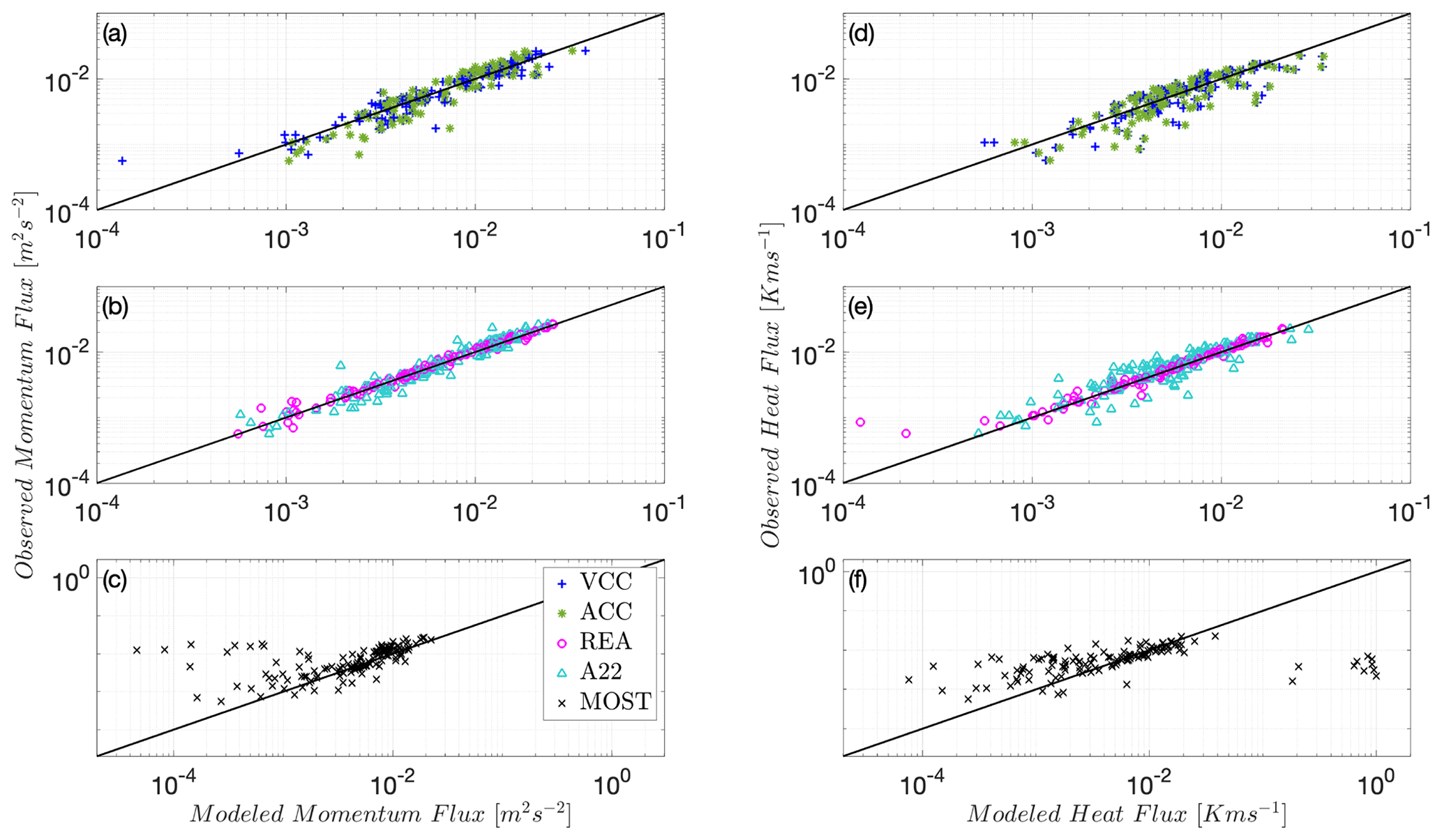
Figure 1 (a–c) Inter-comparison of kinematic momentum fluxes and (d–f) kinematic heat fluxes derived from the various models for the Utqiaġvik site, U09. The 1:1 line is shown as a reference (solid black line). Since both fluxes are negative, they are multiplied by −1 to plot on the log–log scale.

4.2 Simulating a slow scalar sensor for model testing

To address the limited bandwidth of many trace gas sensors, we simulate the output of a real slow sensor $\stackrel{\mathrm{̃}}{s}$ measuring a variable s as the numerical solution to the first-order ODE in Eq. (13). Here, s would be the “fast” turbulent sensor, and $\stackrel{\mathrm{‾}}{\mathrm{\Delta }}$ is the timescale of the filter width (the response timescale of the slow sensor), which we selected to vary in the range [0–5 s] with increments of 1 s. Thus, solving the following equation numerically (using explicit forward Euler time advancement scheme) converts the s time series from 10 Hz to a lower frequency down to 0.2 Hz when $\stackrel{\mathrm{‾}}{\mathrm{\Delta }}$ = 5 s:

$$\begin{array}{}\text{(13)}& {\displaystyle \frac{\mathrm{d}\stackrel{\mathrm{̃}}{s}}{\mathrm{d}t}}+{\displaystyle \frac{\mathrm{1}}{\stackrel{\mathrm{‾}}{\mathrm{\Delta }}}}\stackrel{\mathrm{̃}}{s}={\displaystyle \frac{\mathrm{1}}{\stackrel{\mathrm{‾}}{\mathrm{\Delta }}}}s.\end{array}$$

The observed filtered EC fluxes computed with the filtered scalar signal $\stackrel{\mathrm{̃}}{s}$ are referred to as the LEC fluxes. We also tested another filter type, a low-pass Gaussian filter, and the obtained results were not sensitive to the filter type, but the ODE solution is a more accurate model for a first-order slow-sensing system. The filtering is not applied to the vertical velocity (w) as high-frequency anemometers are readily available. Hence, a tilde denotes the filtered virtual temperature ($\stackrel{\mathrm{̃}}{T_{\mathrm{v}}}$), scalar concentration ($\stackrel{\mathrm{̃}}{s}$), and streamwise velocity ($\stackrel{\mathrm{̃}}{u}$). All three-dimensional velocity components (u, v, and w) are available in high-frequency output of the sonic anemometer, but only u is filtered ($\stackrel{\mathrm{̃}}{u}$) to compare its kinematic momentum fluxes to those of scalars.

In theory, an REA system should not suffer from the slow response of the trace gas sensor since it only requires the mean measurements of $\stackrel{\mathrm{‾}}{s^{+}}$ and $\stackrel{\mathrm{‾}}{s^{-}}$. However, this requires a mechanism to separate the gas streams that has a 10 Hz response time as well. While such systems have been constructed and used, they are typically operated using a certain threshold value that defines a dead-band velocity w₀ below which the system does not switch intake or keeps both intakes closed. This is designed to avoid an excessive number of movements and to guarantee larger individual air samples. In addition, since these systems are typically custom made, there is still a possibility of some latency in the response of the mechanics of some models. In the present implementation, a dynamic dead band that is linked to the turbulence conditions in each period is adopted such that similar amounts of air are sampled in updrafts and downdrafts. We used the empirical finding of Grelle and Keck (2021), as depicted in Eq. (14), which yielded roughly similar amounts of air in the updraft and downdraft reservoirs. Sampling is only activated if the vertical wind exceeds this threshold value in w₀, i.e., |w|>w₀.

$$\begin{array}{}\text{(14)}& w_{\mathrm{0}}={\displaystyle \frac{{\mathit{\sigma }}_{\mathrm{w}}}{\mathrm{3.5}}}\end{array}$$

We should underline the fact that the computations of $\stackrel{\mathrm{‾}}{s^{+}}$ and $\stackrel{\mathrm{‾}}{s^{-}}$ for the REA are first done with the unfiltered s signal (mimicking a flawless and very fast mechanical system), and the dead band of vertical velocity defined above is then the only effective filter that applies to the REA computations. However, when exploring the VEA approach that we will detail later, we will compute the VEA fluxes with $\stackrel{\mathrm{‾}}{s^{+}}$ and $\stackrel{\mathrm{‾}}{s^{-}}$ from the filtered signal produced by Eq. (13).

4.3 LEC, VEA, and A22 model evaluation using simulated slow-sensor data

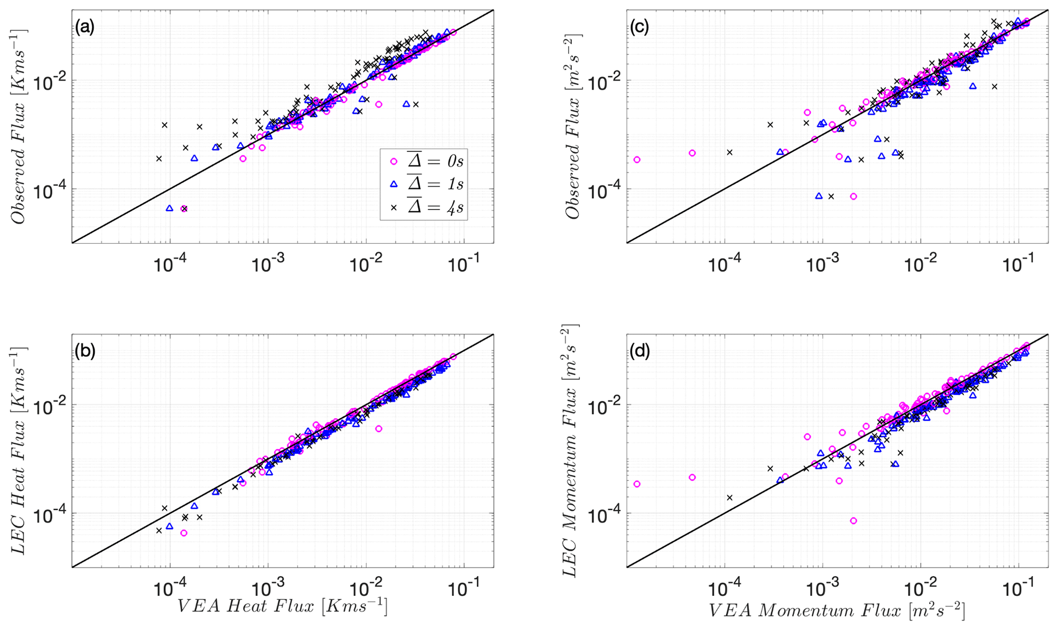
Again focusing on Utqiaġvik data set with its multilevel measurements, the models are now tested using inputs from a slow sensor. The top and middle panel subplots of Fig. 2 show that the LEC and VEA methods significantly, and in similar fashion, underestimate the observed (unfiltered) heat and momentum EC fluxes based on filtered quantities $\stackrel{\mathrm{̃}}{T_{\mathrm{v}}}$ and $\stackrel{\mathrm{̃}}{u}$, respectively, as $\stackrel{\mathrm{‾}}{\mathrm{\Delta }}$ increases. This underestimation, however, is not surprising because under stable conditions small eddies carry a significant proportion of the fluxes, especially when the background flow is laminarizing and intermittent, as shown elsewhere (Ansorge and Mellado, 2014, 2016; Allouche et al., 2022; Issaev et al., 2023). These small eddies are filtered appreciably by the sensor's slow response. We should underline here that an REA system with fast-response mechanical valves will give results equivalent to the unfiltered VEA (VEA recovers an REA system for $\stackrel{\mathrm{‾}}{\mathrm{\Delta }}$ = 0) and will be in good agreement with the actual EC fluxes. However, any latency in the mechanical response of the REA device will introduce some type of filtering to the signal that depends on the device design; this underlines the importance of the mechanical design of these systems. Remarkably, the bottom-panel subplots of Fig. 2c and f show that the A22 model's performance is not sensitive to the signal filtering and provides good estimates of the observed (unfiltered) heat and momentum EC fluxes, even when filtered quantities $\stackrel{\mathrm{̃}}{T_{\mathrm{v}}}$ and $\stackrel{\mathrm{̃}}{u}$ are used, and up to the highest filter width $\stackrel{\mathrm{‾}}{\mathrm{\Delta }}$ = 5 s. The A22 model relies on multilevel means and variances in computing the fluxes, which tend to be carried by larger scales than the actual fluxes; this may explain the independence of the model performance from sensor response.

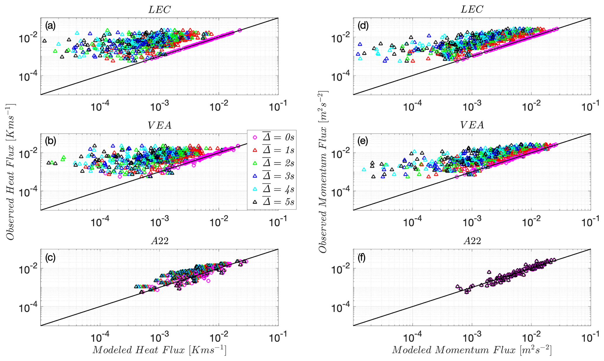
Figure 2 Heat flux using $\stackrel{\mathrm{̃}}{T_{\mathrm{v}}}$ predicted by LEC (a), VEA (b), and A22 (c) models and momentum flux using $\stackrel{\mathrm{̃}}{u}$ predicted by LEC (d), VEA (d) and A22 (f) models at the Utqiaġvik site, U09, compared to real observed EC fluxes. The 1:1 line is shown as a reference (solid black line). Both fluxes are negative and are thus multiplied by −1 to plot on the log–log scale. $\stackrel{\mathrm{‾}}{\mathrm{\Delta }}\left(s\right)$ is the filter timescale.

Given the results above, a followup question is whether the VEA model estimates with a filtered signal actually correspond to the fluxes that would be computed using eddy covariances of the filtered scalar signal, i.e., the LEC fluxes. Figure 3a and b indeed show that the VEA model is still a reliable method to capture these filtered observed heat and momentum LEC fluxes at Utqiaġvik as $\stackrel{\mathrm{‾}}{\mathrm{\Delta }}$ increases. All quantities here, including the fluxes, are computed based on filtered series $\stackrel{\mathrm{̃}}{T_{\mathrm{v}}}$ and $\stackrel{\mathrm{̃}}{u}$. This implies that VEA flux estimates are broadly comparable to the filtering of the LEC fluxes by slow-response scalar sensors.

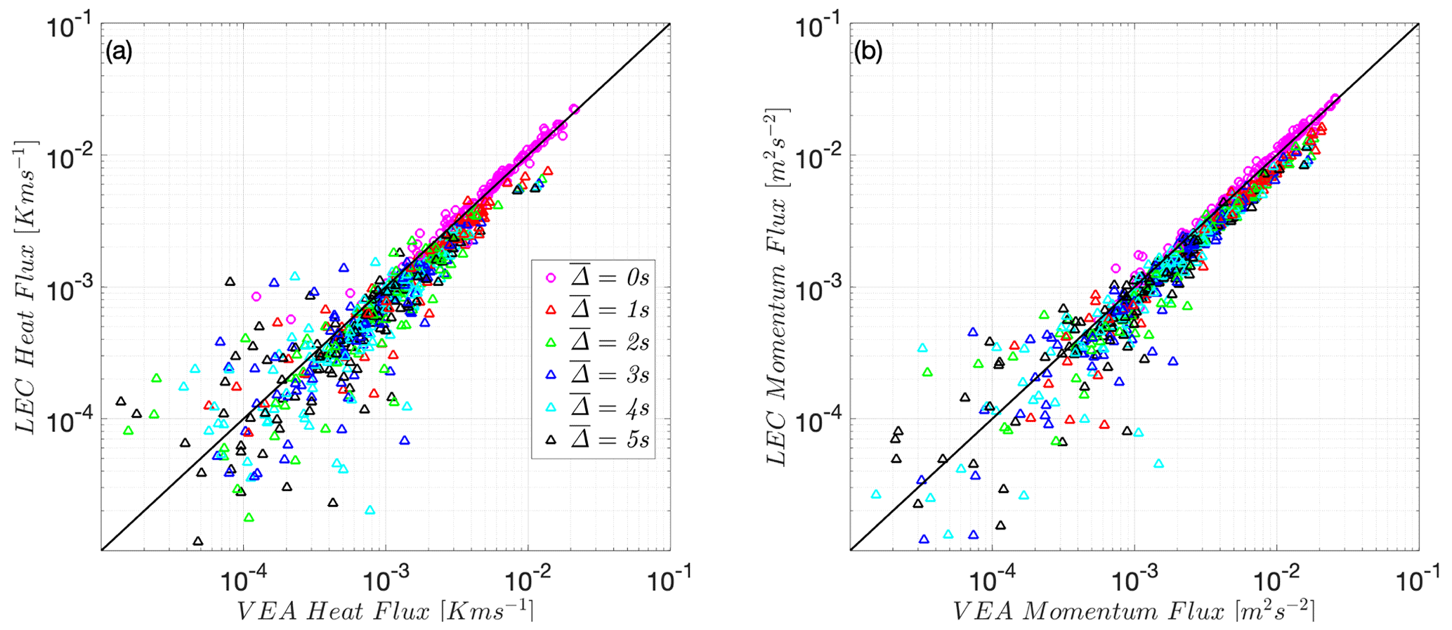
Figure 3 (a) Heat flux using $\stackrel{\mathrm{̃}}{T_{\mathrm{v}}}$ predicted by the VEA model versus the filtered observed heat LEC flux and (b) momentum flux using $\stackrel{\mathrm{̃}}{u}$ predicted by the VEA model versus the filtered observed momentum LEC flux at the Utqiaġvik site, U09. The 1:1 line is shown as a reference (solid black line). Both fluxes are negative and are thus multiplied by −1 to plot on the log–log scale. $\stackrel{\mathrm{‾}}{\mathrm{\Delta }}$ is the timescale filter width (s).

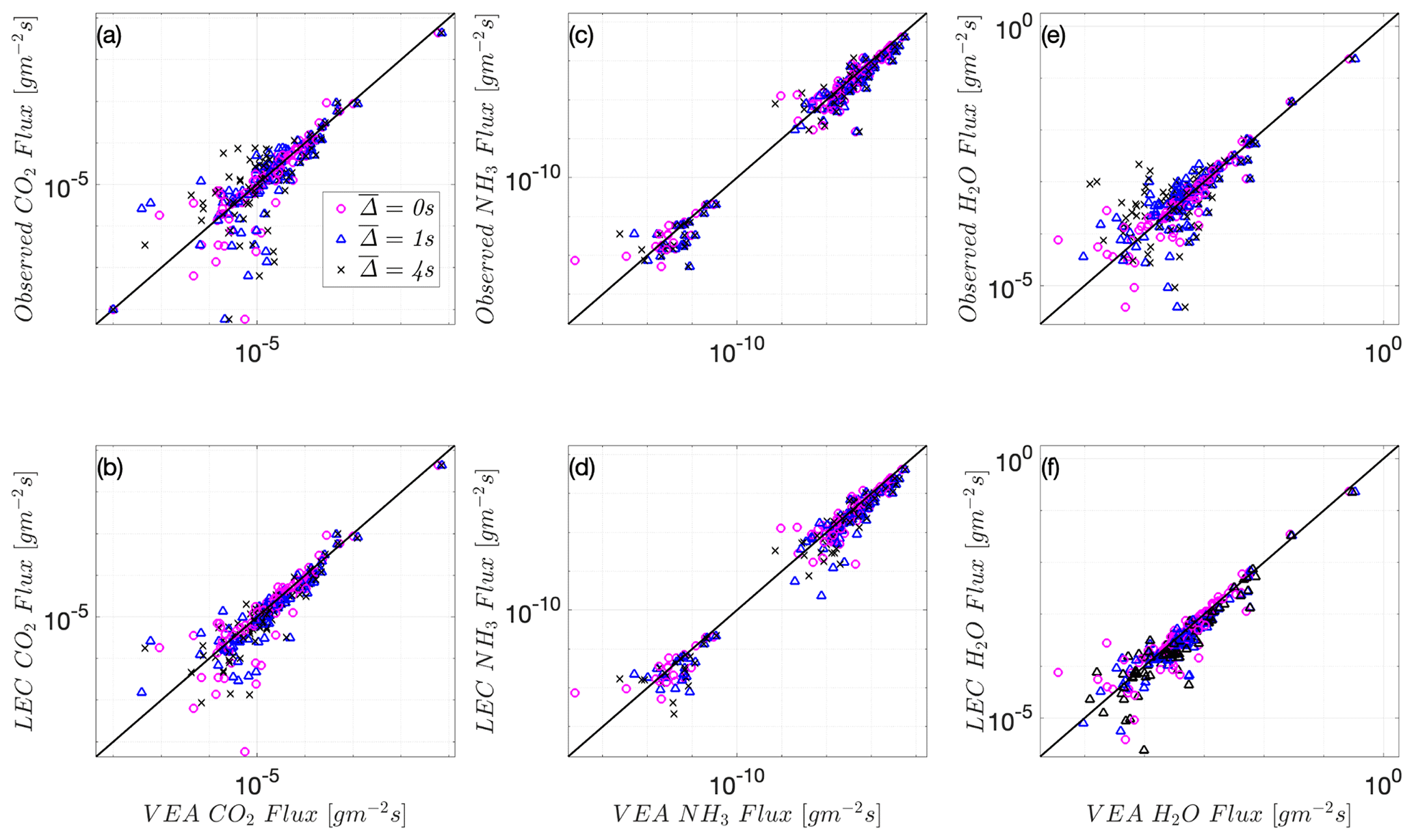
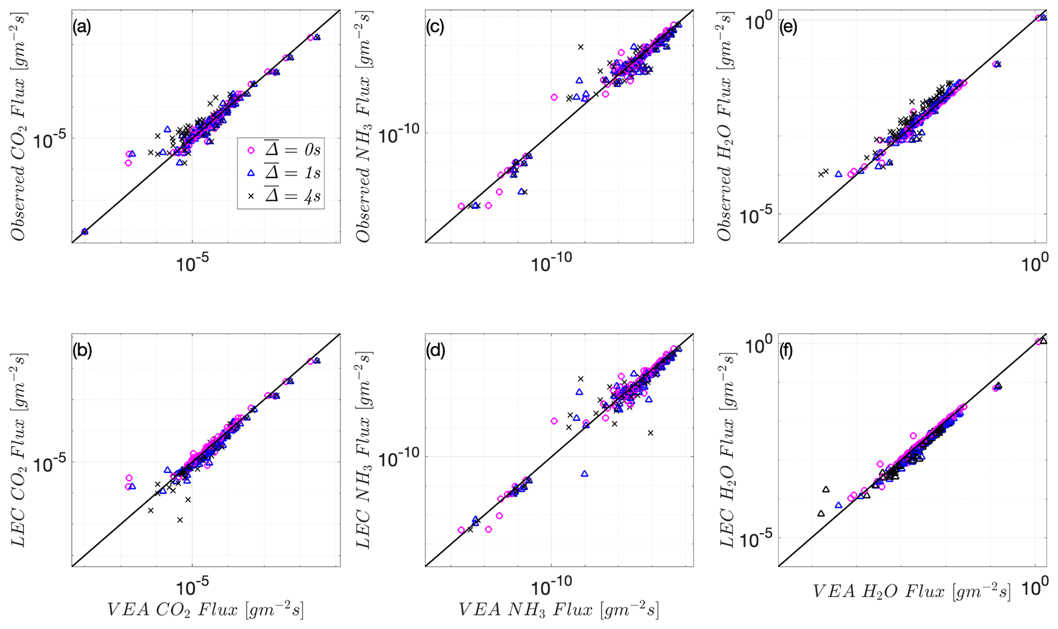
This match between VEA and LEC fluxes is also observed at the Wendell site for heat and momentum, as well as for the other scalars available at that site (CO₂, NH₃, and H₂O). As in Utqiaġvik's site, Figs. 4b, d and 5b, d, and f show that VEA performs better when evaluated against the LEC fluxes, compared to Figs. 4a, c and 5a, c, and e that compare it to total EC fluxes. Note that since only one level of measurements at Wendell is available, gradients of first-order moments could not be computed, which precludes testing of MOST or A22 models.

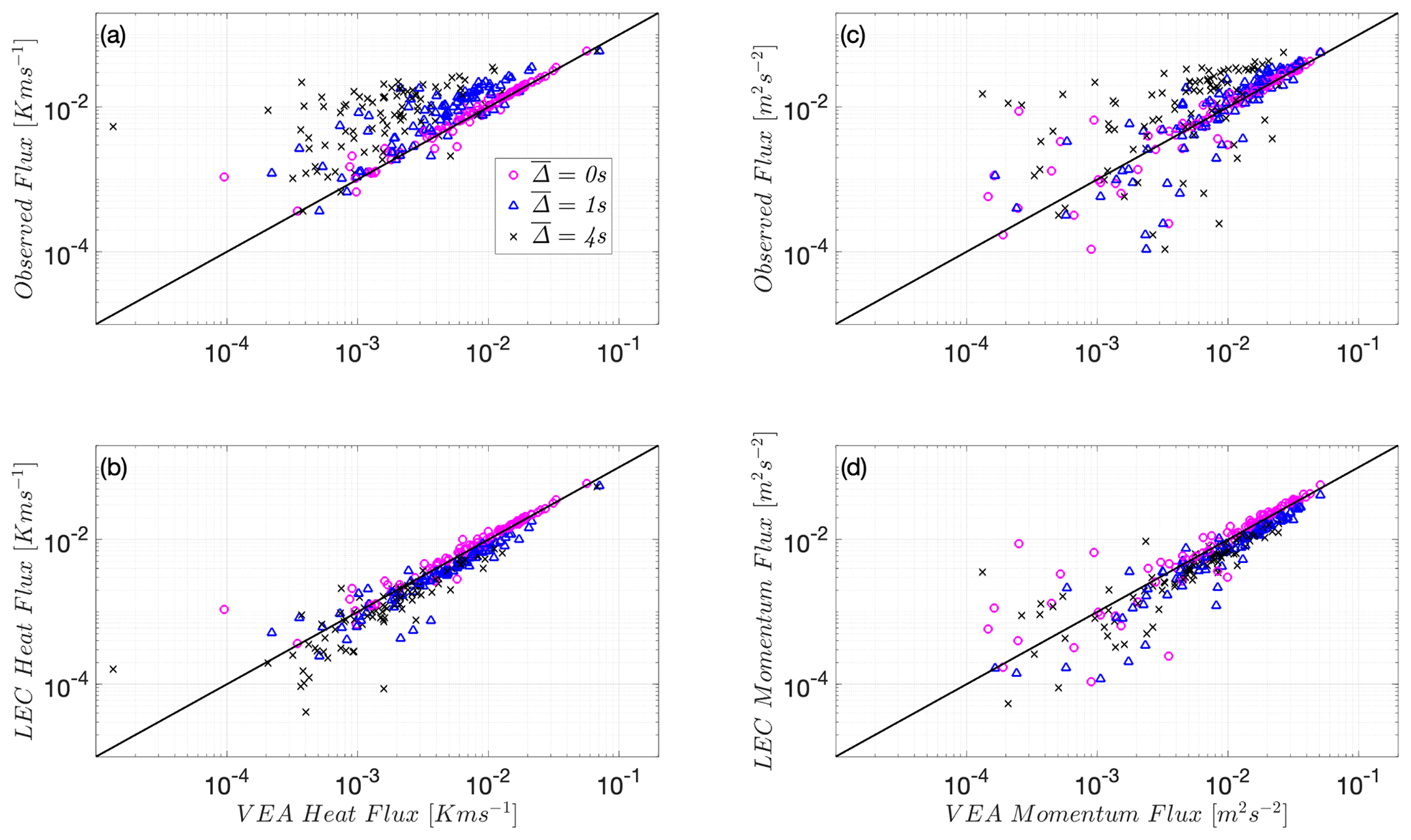
Figure 4 Heat flux using $\stackrel{\mathrm{̃}}{T_{\mathrm{v}}}$ predicted by VEA versus the observed unfiltered EC flux (a) and the filtered LEC flux (b) and momentum flux using $\stackrel{\mathrm{̃}}{u}$ predicted by VEA versus the observed unfiltered EC flux (c) and filtered LEC flux (d) at the Wendell site, W22. The 1:1 line is shown as a reference (solid black line). Both fluxes are multiplied by −1 to plot on the log–log scale. $\stackrel{\mathrm{‾}}{\mathrm{\Delta }}$ is the timescale filter width (s).

Figure 5 Similar to Fig. 4 but here for scalars, (a, b) CO₂, (c, d) NH₃, and (e, f) H₂O.

These similar VEA findings among the two different sites indicate that, under stable conditions, the VEA captures the fluxes of the “resolved” eddies. Any slow-response filtering will cause the method to significantly underestimate the needed high-frequency, full observed fluxes. An important question (addressed in the next subsection) that follows is whether the VEA fluxes can be “corrected” under stable conditions to recover the missed fluxes. The proposed modifications, outlined below for the VEA methodological framework, offer a correction for VEA flux estimates to recover their corresponding total EC fluxes. It is to be noted that under unstable conditions at the Wendell site, where flux carrying eddies are of much larger scales than under stable conditions, the VEA method is found to be almost insensitive to the considered filter widths ($\stackrel{\mathrm{‾}}{\mathrm{\Delta }}$'s) (refer to Appendix A). Therefore, VEA performs well and captures the observed (high- and low-frequency) fluxes under unstable convective regimes, and hence biases in predicting scalar fluxes are expected to be minimal (Figs. A1 and A2). This also implies that for conventional REA, the mechanical response speed is not as critical under unstable conditions. In the next subsection, we aim to develop an effective correction for the under-resolved fluxes under stable conditions that will provide a method to obtain continuous accurate fluxes using VEA over the whole diurnal cycle.

4.4 A sensor-response correction for the optimal VEA coefficient β_v

Figure 3 reveals that the scatter between VEA and EC or LEC results is larger when the fluxes are small, which would translate into larger errors and scatter in the values of β_s. Analyses not shown here also reveal that β_s values calculated for each period converge well towards the 0.59 value when the correlation R_ws increases; i.e., R_ws > 0.2, indicating larger fluxes, with more scatter for lower correlation values. However this scatter is randomly distributed around the 1:1 line, indicating some error cancellation when the fluxes are integrated over longer periods of time. Discussions on these random variations in β_s have linked them to the effect of height above canopies (Gao, 1995) and to the energy content influence of the associated eddy motions (Katul et al., 1996), among others, and are not a focus of the present paper.

Figures 2a and d and 4a and c, on the other hand, reveal that the chosen value of β_s = 0.59 in the modeled fluxes is a good estimate in recovering the observed EC fluxes when the signal is not filtered ($\stackrel{\mathrm{‾}}{\mathrm{\Delta }}$ = 0 s). Missing smaller eddies (when the signal is filtered) that contribute significantly to fluxes under stable, but not unstable, conditions thus requires a larger β_s to predict the correct fluxes using VEA. Such underestimation was attributed to the filtering operation, dictated here by the choice of $\stackrel{\mathrm{‾}}{\mathrm{\Delta }}$. This motivates a model development for β_s that incorporates the effect of filtering of the fast eddies, which we will express as β_v.

Furthermore, the agreement between the LEC and VEA predictions when the scalar signal is filtered also opens the possibility of applying the VEA method as a surrogate for REA, without an actual device that separates air streams from downdrafts and updrafts. If a slow-response sensor (open- or closed-path) is available, the VEA method that uses the REA equation (Eq. 6) can be applied, with $\stackrel{\mathrm{‾}}{s^{+}}$ and $\stackrel{\mathrm{‾}}{s^{-}}$ computed using conditional averaging of the scalar time series based on the sign of w – similar to what is done to the simulated REA measurements – but without the dead band given in Eq. (14).

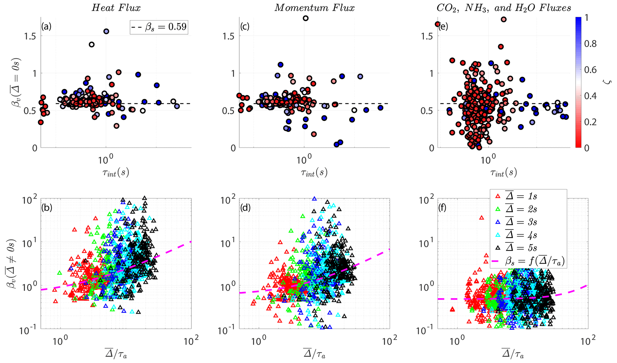
Figure 6 (a, c, e) Scatter of the computed β_s for the observed (unfiltered) heat, momentum and passive scalar (CO₂, NH₃, and H₂O) fluxes at both sites relative to the integral timescale τ_int(s), respectively. Panels (b), (d), and (f) show the similarly computed β_v for the respectively observed (filtered) fluxes relative to $\stackrel{\mathrm{‾}}{\mathrm{\Delta }}/{\mathit{\tau }}_{\mathrm{a}}$. τ_a is an advective timescale, and the solid magenta lines refer to the empirical fit models ${\mathit{\beta }}_{\mathrm{v}}=a{\left(\stackrel{\mathrm{‾}}{\mathrm{\Delta }}/{\mathit{\tau }}_{\mathrm{a}}\right)}^b+c$; refer to Table 1.

For this purpose, we first compute each period's optimal β_v (i.e., by inverting the expression in Eq. 6) that causes the REA-predicted fluxes, equivalent to VEA computed with the raw signal without filtering, to match the exact observed fluxes when $\stackrel{\mathrm{‾}}{\mathrm{\Delta }}$ = 0 s (no filtering) across the two contrasting sites. The top-panel subplots, Fig. 6a for heat, Fig. 6c for momentum, and Fig. 6e for all three passive trace gases (CO₂, NH₃, and H₂O), show a scatter plot of these exact β_v's relative to the integral timescale τ_int(s) for each period's co-spectrum, where the data points are colored with the MOST stability parameter. The integral timescale (τ_int) is determined by integrating the autocorrelation function (${\mathit{\rho }}_{w^{\prime }{s}^{\prime }}\left(\mathit{\tau }\right)$) up to the first zero-crossing from the measured $w^{\prime }{s}^{\prime }$ instantaneous time series. We observe β_v values that depart from β_s = 0.59 under all stabilities, but in general there is no clear β_v dependence on τ_int as depicted here.

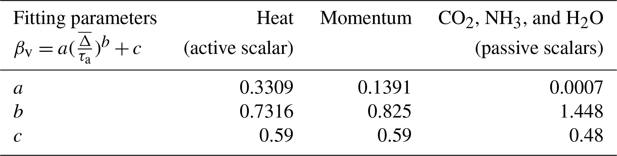
Table 1 Proposed models incorporating both sites, Utqiaġvik (U09) and Wendell (W22), with the dead-band criterion accounted for and ${\mathit{\beta }}_{\mathrm{v}}=a{\left(\frac{\stackrel{\mathrm{‾}}{\mathrm{\Delta }}}{{\mathit{\tau }}_{\mathrm{a}}}\right)}^b+c$, $c={\mathit{\beta }}_{\mathrm{v}}(\stackrel{\mathrm{‾}}{\mathrm{\Delta }}=\mathrm{0})={\mathit{\beta }}_{\mathrm{s}}$.

For $\stackrel{\mathrm{‾}}{\mathrm{\Delta }}\ne \mathrm{0}$ s, the corresponding bottom-panel subplots, Fig. 6b, d, and f, show these same β_v's relative to $\stackrel{\mathrm{‾}}{\mathrm{\Delta }}/{\mathit{\tau }}_{\mathrm{a}}$ for different $\stackrel{\mathrm{‾}}{\mathrm{\Delta }}$'s, where τ_a is an advective timescale. After experimenting with various choices of timescales for normalizing the filter scale $\stackrel{\mathrm{‾}}{\mathrm{\Delta }}$, an advective timescale formed by z and $\stackrel{\mathrm{‾}}{u}$, hereafter labeled as ${\mathit{\tau }}_{\mathrm{a}}=(\mathit{\kappa }z/\stackrel{\mathrm{‾}}{u})$, appears to provide the best scaling for the variations of β_v with the filter size (κ is the von Kármán constant). This converges with the work of Horst (1997), who formulated corrections to estimate the attenuation of scalar flux measurements by the slow response of sensors (akin to LEC). They used the sensor response frequency and a normalized frequency formulated based on τ_a, which is the frequency of the peak of the logarithmic cospectrum $f_{\mathrm{m}}=n_{\mathrm{m}}\mathit{\kappa }/{\mathit{\tau }}_{\mathrm{a}}$, to correct for the missed fluxes. In that work, n_m is the dimensionless frequency at the cospectral maximum, where it is estimated from observations of its behavior as a function of atmospheric stability ζ. The advective timescale was similarly found to be a plausible choice in describing the drift and non-linear diffusion terms of a proposed non-linear Langevin equation to model the turbulent kinetic energy in stably stratified ABL (Allouche et al., 2021). This characteristic timescale, τ_a, measures the advection time of the attached eddies, of size κz, past a fixed sensor.

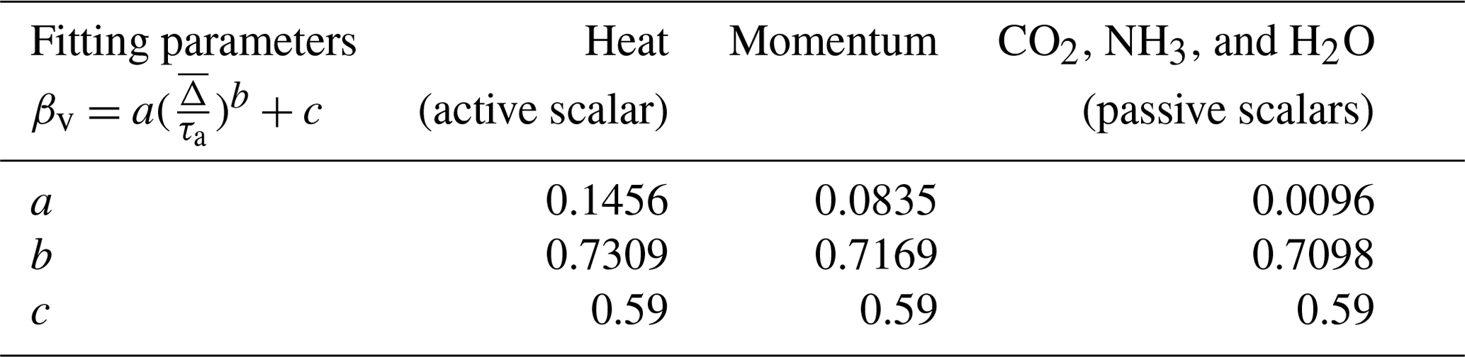
As depicted in Fig. 6, an empirical fit that relates β_v to $\stackrel{\mathrm{‾}}{\mathrm{\Delta }}/{\mathit{\tau }}_{\mathrm{a}}$ i.e., ${\mathit{\beta }}_{\mathrm{v}}=f(\stackrel{\mathrm{‾}}{\mathrm{\Delta }}/{\mathit{\tau }}_{\mathrm{a}})$, is proposed here to recover the real observed (unfiltered) EC fluxes using the VEA method with ($\stackrel{\mathrm{̃}}{s}$) measurements. This relation is best described using a power-law model, ${\mathit{\beta }}_{\mathrm{v}}=a(\stackrel{\mathrm{‾}}{\mathrm{\Delta }}/{\mathit{\tau }}_{\mathrm{a}}{)}^b+c$, and Table 1 summarizes these empirical coefficients (a,b) for momentum, heat (active scalar), and passive scalar (CO₂, NH₃, and H₂O) fluxes at both sites, where $c={\mathit{\beta }}_{\mathrm{v}}(\stackrel{\mathrm{‾}}{\mathrm{\Delta }}=\mathrm{0})={\mathit{\beta }}_{\mathrm{s}}$. The reported b exponent for all fluxes, which describes how β_v scales with $\stackrel{\mathrm{‾}}{\mathrm{\Delta }}/{\mathit{\tau }}_{\mathrm{a}}$, varies between active and passive scalars. Note that if the dead-band criterion is removed, b ≈ 0.7 and does not vary much among all scalars as shown in Table 2, hinting at the possible universality of such dependence for a VEA model that removes the need for a complex mechanical REA system. Nevertheless, further exploration at disparate sites and analyses of observational data for different scalars across wider stability ranges and different non-ideal surfaces are needed to have increased statistical confidence in the reported values of (a,b) and their generalizability, especially for the Utqiaġvik site, which does not have measurements of the passive scalars.

Table 2 Proposed models incorporating both sites Utqiaġvik (U09) and Wendell (W22) without accounting for the dead-band criterion, ${\mathit{\beta }}_{\mathrm{v}}=a(\frac{\stackrel{\mathrm{‾}}{\mathrm{\Delta }}}{{\mathit{\tau }}_{\mathrm{a}}}{)}^b+c$, $c={\mathit{\beta }}_{\mathrm{v}}(\stackrel{\mathrm{‾}}{\mathrm{\Delta }}=\mathrm{0})={\mathit{\beta }}_{\mathrm{s}}$.

A common feature for all fluxes, as depicted in the bottom panel of Fig. 6, is that the proposed model becomes less certain as $\stackrel{\mathrm{‾}}{\mathrm{\Delta }}$ increases (as expected). Therefore, such a model becomes less reliable with very slow sensors that cannot resolve most of the scales of turbulence and is ideally suited for moderately slow sensors that can still resolve the larger eddies. Otherwise, to compute β_v, the only needed inputs are (i) $\stackrel{\mathrm{‾}}{\mathrm{\Delta }}$ (ideally provided by the slow-sensor manufacturer) and (ii) τ_a (computed from mean wind measurements). The reported fitting parameters in Table 1 are obtained using the least absolute residual (LAR) method, so that extreme values, which occur less frequently and may be related to unusual conditions or measurement errors, have a lesser influence on the fit. Given the variability in the optimal values of β_v, the proposed models would be mostly suited for quantification of long-term aggregates (net averaged fluxes) of the scalars cycle.

5 Conclusions

Conventional and novel formulations are assessed to predict scalar fluxes under stable conditions. These conditions pose measurement challenges because the turbulence timescales are shorter, thereby amplifying the effects of any spatial or temporal averaging by sensors – or even instrument separation between w^′ and c^′. The models tested include the MOST-based flux–gradient model; the A22 gradient- and variance-based flux model; the conventional REA approach; and VEA, a virtual version of REA requiring no flow separation and collection device that can be used with moderately slow gas sensors. The test used measurements collected at two different sites (Utqiaġvik and Wendell).

It was found that the REA and A22 models outperform the conventional models (e.g., MOST) and are thus less sensitive to departures from ideal flow conditions of homogeneity, steadiness, negligible vertical transport of covariances, and TKE production–dissipation balance. The A22 model was also found to perform well and provide good estimates of the observed (unfiltered) heat and momentum EC fluxes, even when filtered quantities $\stackrel{\mathrm{̃}}{T_{\mathrm{v}}}$ and $\stackrel{\mathrm{̃}}{u}$ are used and up to the highest filter width $\stackrel{\mathrm{‾}}{\mathrm{\Delta }}$ = 5 s. This is because the A22 model is insensitive to filtering operations of the turbulent scales as it relies on multilevel means and variances in computing the fluxes, which tend to be carried by larger scales than the actual fluxes; this may explain the independence of the model performance from sensor response.

The REA model, on the other hand, would be sensitive to any latency in the response of the mechanical air flow separation system but is not affected by the w₀ dead band. This underlines the importance of the design and construction of REA devices, which remain inaccessible commercially and are rather custom-made by researchers who use them. This prompted us to examine the possibility of using a virtual eddy accumulation (VEA) version where separating the updrafts and downdrafts to obtain the conditional mean concentrations needed for REA is done digitally, only using the sign of w and without a need for a mechanical device.

With numerically simulated slow sensors, however, it was noted that the A22 model outperforms VEA in predicting the observed (unfiltered) EC fluxes. VEA was instead reproducing the EC fluxes computed with a filtered scalar signal, which we called the large-eddy-covariance (LEC) fluxes here. This suggests that a VEA approach can plausibly be utilized without a physical device to separate the updraft and downdraft air streams but requires a correction for the missed (filtered) scales. To correct the underestimated VEA fluxes, relative to the observed (unfiltered) EC fluxes, a model for the β_v coefficients of the VEA model that incorporates the effect of filtering is proposed. The results indicate that the corrected VEA model remains robust in terms of reproducing long-term averages of the scalar fluxes across their ecosystem lifetime cycle but becomes less certain over individual periods as the sensors response time $\stackrel{\mathrm{‾}}{\mathrm{\Delta }}$ increases. Use of this model, along with the observations reported in Appendix A that reveal an insensitivity of β_v to sensor response under unstable regimes (β_v=β_s), suggests that VEA can be a robust framework for estimating turbulent fluxes when only single-level measurements are available but with sensors that can still resolve the larger scales of turbulence (i.e., with response frequencies ≈ 0.5 to 1 Hz). The A22 can be alternatively used, under stable conditions, when multilevel measurements are available to compute needed mean gradients, even with slow-response sensors.

Appendix A: VEA performance under unstable conditions at Wendell

Figures A1 and A2 show the same plots as Figs. 4 and 5, respectively, but here under unstable conditions. As seen here, VEA is insensitive to filtering operations.

Figure A1 Similar to Fig. 4 but under unstable conditions.

Figure A2 Similar to Fig. 5 but under unstable conditions.