Aerosol optical properties within the atmospheric boundary layer predicted from ground-based observations compared to Raman lidar retrievals during RITA-2021

In this study, we utilised ground-based in situ measurements of the aerosol chemical composition and particle size distribution, along with meteorological data from the European Centre for Medium-Range Weather Forecasts (ECMWF), to predict vertical profiles of aerosol optical properties, including the aerosol scattering coefficient, backscatter coefficient, extinction coefficient, and lidar ratio. The predicted ambient profiles were compared to retrievals by a multi-wavelength Raman lidar during the Ruisdael Land–Atmosphere Interactions Intensive Trace-gas and Aerosol (RITA) campaign in the Netherlands in 2021 for 26 time periods of approximately 1 h each. Predicted and retrieved extensive aerosol properties (scattering, backscatter, and extinction coefficient) were comparable only approximately 35 % of the time, mostly under the condition of well-mixed boundary layers. In this case, ground-based measurements can provide a way to extend extinction profiles to lower altitudes, where they cannot be retrieved, and to verify the lidar-measured profiles. Accurate representation of hygroscopic growth is required for adjusting the dry size distribution to ambient size distribution, and the estimated relative humidity profile may have a substantial influence on the shape of the calculated profiles. On the other hand, the lidar ratio profiles predicted by ground-based data also compared reasonably well to the retrieved lidar profiles (starting at 800 m) for conditions where the predicted and retrieved backscatter profiles differed considerably. The difference in the predicted and retrieved lidar ratio is usually less than ±30 %. Our study thus shows that, for well-mixed boundary layers, a representative lidar ratio can be estimated from ground-based in situ measurements of chemical composition and dry size distribution. This approach offers a method of providing lidar ratios calculated from independent in situ measurements for simple backscatter lidars or at times when Raman lidar profiles cannot be measured (e.g. during the daytime). It only uses data that are routinely available at aerosol measurement stations and is therefore not only useful for further validating lidar measurements but also for bridging the gap between in situ measurements and lidar remote sensing.

1 Introduction

Aerosols play an important role in climate change by altering the Earth's radiation budget through their interaction with solar radiation. Aerosols reflect part of the sunlight, thereby reducing the radiation at the Earth's surface (Twomey, 1977; IPCC, 2013), which results in a cooling effect. On the other hand, certain types of aerosols can also absorb solar radiation, which locally warms the atmosphere and results in a change in the temperature profile, further affecting atmospheric circulations (Koren et al., 2008; Rosenfeld et al., 2014; Bréon, 2006). In addition, aerosol particles can act as cloud condensation nuclei or ice nuclei affecting the microphysical properties of clouds, thereby affecting the radiation budget indirectly (Graf, 2004; Lohmann and Feichter, 2005; Bréon, 2006). There are still large uncertainties in predicting the contribution of aerosol radiative forcing to climate change, due to the complexity of microphysical and chemical processes and their dynamic feedback on the aerosol budget (Kaufman et al., 2005; Feingold et al., 2001; Graf, 2004). To reduce the uncertainties, observation and simulation of aerosol optical properties and their vertical profiles are essential for a better understanding of aerosol radiative forcing (Moise et al., 2015; Chang et al., 2006).

Light detection and ranging (lidar) is a widely used active remote-sensing method for studying the spatial distribution of aerosol optical properties (Collis and Russell, 1976; Measures, 1984; Whiteman et al., 1992; Weitkamp, 2005). The detected signal of the elastically backscattered light can be converted into the backscatter and extinction coefficients based on an analytical solution of the so-called “lidar equation” (Klett, 1981; Fernald, 1984) with the assumption of a given extinction-to-backscatter ratio, called the “lidar ratio”. However, the lidar ratio is governed by many factors, such as the wavelength of incoming light, the aerosol chemical composition, particle size distribution, relative humidity, and other atmospheric conditions (Salemink et al., 1984; Floutsi et al., 2023). Large errors can occur when retrieving aerosol extinction from backscattered signals. Thus, a Raman lidar technique based on Raman spectroscopy was developed to address this problem (Ansmann et al., 1990). The profiles of the backscatter and the extinction coefficient can be determined independently by the Raman lidar without the assumption of a lidar ratio (Ansmann et al., 1992a, b). However, a common limitation on the accuracy of the lidar-based retrievals emerges for distances close to the instrument, where only a fraction of the atmospheric volume illuminated by the laser pulse is within the lidar's receiver field of view, resulting in a “blind zone” at the instrument (no overlap) and a region that gradually becomes visible for the receiver after some distance (incomplete overlap region) (Wandinger and Ansmann, 2002). While Raman backscatter retrievals are less affected by the incomplete overlap region, Raman extinction and elastic lidar retrievals are particularly sensitive to it, even after an overlap correction is applied, and thus can only accurately record the aerosol profiles above a certain altitude (Hervo et al., 2016; Wandinger and Ansmann, 2002).

Besides active remote sensing, vertical aerosol profiles can also be measured by in situ airborne instruments (Düsing et al., 2021, 2018; Haarig et al., 2019). These give more accurate information, but they are expensive and time-consuming and thus lack the temporal coverage of lidar measurements. They are essential in the evaluation of the lidar retrievals, and several studies have modelled aerosol optical vertical profiles based on Mie theory using vertically resolved aerosol information but measured by airborne instruments (Düsing et al., 2021, 2018; Ferrero et al., 2019). Their results support the usefulness of in situ observations for the evaluation of lidar retrievals; however, there are only a few profiles available due to the high cost of airborne measurements.

In this study, we evaluate a method to predict vertical profiles of aerosol optical properties using ground-based in situ measurements of aerosol chemical composition and particle size distribution combined with meteorological profiles from the European Centre for Medium-Range Weather Forecasts (ECMWF). The experiments were performed at the Cabauw Experimental Site for Atmospheric Research (CESAR) site in the Netherlands during the Ruisdael Land–Atmosphere Interactions Intensive Trace-gas and Aerosol (RITA) 2021 field campaign (https://ruisdael-observatory.nl/the-rita-2021-campaign/, last access: 20 July 2022). The primary goal of this study is to evaluate if routine ground-based measurements can be used to predict the lidar ratio and the extinction coefficient in the region of incomplete overlap between the laser beam and the receiver field of view of the lidar detector system, where it cannot be retrieved by the Raman lidar. If successful, this information can then be used to extrapolate extinction profiles to the ground or to derive extinction data from elastic backscatter lidars. A further goal is to explore under which circumstances the aerosols measured on the ground can represent the vertical aerosol distribution in the atmosphere. The advantage of the proposed method is that we use only ground-based data, which are readily available at most lidar sites, and the easily obtained ECMWF data. In the subsequent section, we describe the in situ measurements and the calculations used in this study. The third section presents an evaluation of the calculated optical properties against nephelometer measurements at ground level. Subsequently, calculated vertical profiles of the optical properties are compared to lidar retrievals in three case studies, representing polluted and clean conditions. Finally, a comparison between calculated and retrieved lidar ratios is presented for all Raman lidar measurement periods.

2 Methods

2.1 Experiment site and campaign description

The RITA campaign was carried out at CESAR in the Netherlands (51.97° N, 4.93° E) during spring (11–24 May) and during autumn (16 September–12 October) in 2021. CESAR is one of the core observatories for the Ruisdael observatory (https://ruisdael-observatory.nl/, last access: 20 July 2022) and is also part of the Aerosols, Clouds, and Trace Gases Research Infrastructure (ACTRIS; http://actris.net/, last access: 20 July 2022) and Integrated Carbon Observation System (ICOS; https://www.icos-cp.eu/, last access: 20 July 2022). An aerial view of the infrastructure setup during the RITA campaign and the CESAR location are shown in Fig. 1. The site is situated in a polder 0.7 m below average sea level and surrounded by a flat pasture landscape. The mode of the wind direction distributions was southwest, but winds also came from the northeast, so the potential pollution sources could be from Rotterdam, with its large international harbour, but also from nearby Utrecht. The ground-based aerosol in situ measurements included the aerosol chemical composition, particle size distribution, and aerosol optical properties. The remote-sensing observations by the Raman lidar were obtained regularly during the campaign depending on the atmospheric conditions.

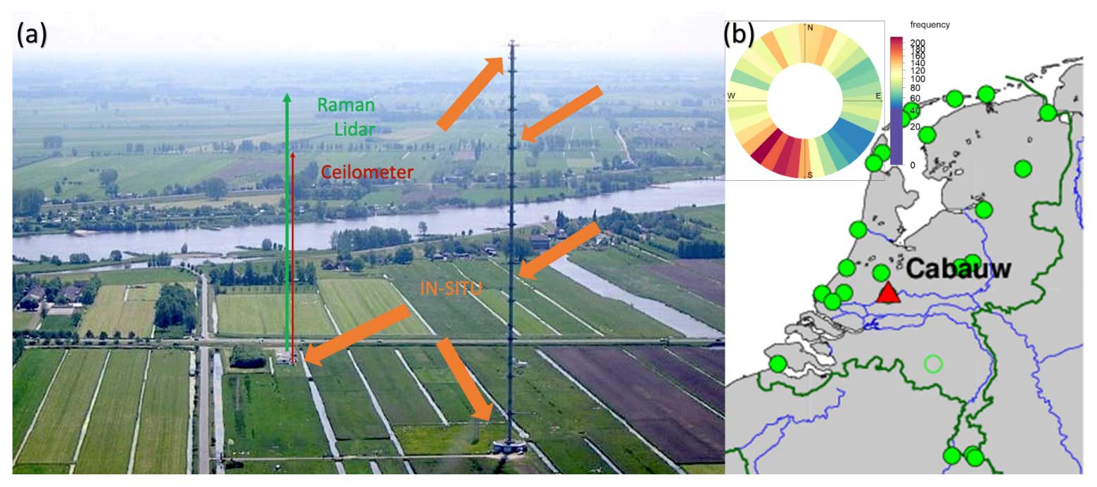
Figure 1 (a) An aerial view of the infrastructure setup during the RITA-2021 campaign (photo by Wouter Knap, KNMI). (b) The frequency of the hourly average wind direction at CESAR during the RITA campaign from 7 May to 20 October 2021 and the site location (marked in red) in the Netherlands (http://gnss1.tudelft.nl/dpga/station/Cabauw.html, last access: 20 July 2022).

2.1.1 Aerosol chemical composition measurements

Aerosol chemical composition was measured by different online and offline methods during the campaign.

• (i)

  A time-of-flight aerosol chemical speciation monitor (TOF-ACSM; Aerodyne Research Inc., Billerica, MA) equipped with a capture vaporiser (CV) and a PM_2.5 lens measured the mass concentration of non-refractory chemical compounds with a 10 min time resolution. The TOF-ACSM was installed in a trailer, which was next to the remote-sensing site as shown in Fig. 1a, approximately 200 m from the other in situ measurements. The inlet was a Teflon-coated aluminium cyclone (URG 2000-30ED) with an aerodynamic cut-off diameter of 2.5 µm at ambient conditions, and the inlet flow rate was 2.3 L min⁻¹ controlled by an ARI sample line flow controller (S/N FCB-023) at the head of the TOF-ACSM inlet. Particles were dried by a Nafion dryer (Perma Pure, New Jersey). Five chemical species, namely ammonium (${{\mathrm{NH}}_{\mathrm{4}}}^{+}$), nitrate (${{\mathrm{NO}}_{\mathrm{3}}}^{-}$), sulfate (${{\mathrm{SO}}_{\mathrm{4}}}^{\mathrm{2}-}$), chloride (Cl⁻), and organics (Org), were derived based on the fragmentation tables for the TOF-ACSM (Fröhlich et al., 2013). The standard calibrations, such as the flow rate calibration, lens calibration, and heater bias (HB) voltage tuning, were performed before and after the campaign. Ionisation efficiency (IE) and the relative ionisation efficiency (RIE) were determined by calibration with NH₄NO₃ and (NH₄)₂SO₄ solutions with a concentration of 0.005 mol L⁻¹. The calibration values used in this study are IE NO₃=258.20 pg s⁻¹, RIE NH₄=3.51, RIE SO₄=1.33, RIE Org=1.40, RIE Chl=1.30, at an air beam $\left(\text{AB}\right)=\mathrm{4.55}\times {\mathrm{10}}^{\mathrm{5}}$ ions s⁻¹, and flow rate=1.46 cm³ s⁻¹. The data were processed by Tofware software (version 3.2.4; Tofwerk AG, Thun, Switzerland).

• (ii)

  PM_2.5 and PM₁₀ filter samples were collected for 24 h using a SEQ47/50 (Leckel GmbH, Germany) instrument with a sequential low-volume system (LVS) of 2.3 m³ h⁻¹ next to the trailer with the TOF-ACSM. The sampler operation was based on the European Standards (EN12341: 1998 and EN14907: 2005). The filter samples were collected under ambient conditions, stored at approximately −20 °C, and protected using ice packs during transportation. The concentrations of three inorganic anions (${{\mathrm{NO}}_{\mathrm{3}}}^{-}$, Cl⁻, ${{\mathrm{SO}}_{\mathrm{4}}}^{\mathrm{2}-}$) and five cations (Na⁺, K⁺, Mg²⁺, Ca²⁺, ${{\mathrm{NH}}_{\mathrm{4}}}^{+}$) were determined by chromatography (ICS-1100, Thermo Scientific). Organic carbon (OC) and elemental carbon (EC) were analysed by a Sunset thermal optical analyser (TOA; Sunset Laboratory Inc.) using the EUSAAR2 protocol (Cavalli et al., 2010; Karanasiou et al., 2020). The details of the data evaluation can be found in Liu et al. (2024).

• (iii)

  The equivalent black carbon (eBC) mass concentration was measured by a multi-angle absorption photometer (MAAP model 5012, Thermo Fisher Scientific Inc., Franklin, MA) with 5 min time resolution (Petzold and Schönlinner, 2004; Petzold et al., 2005). A constant scattering cross-section value (6.6 m² g⁻¹) based on the user handbook was given for converting the aerosol light absorption coefficient at 670 nm.

  The MAAP and the other in situ measurements discussed below were installed in the Cabauw main building underneath the 213 m high tower, as displayed in Fig. 1. The MAAP performed measurements behind a PM₁₀ inlet that was situated on the roof, 4.5 m above the ground. A wide-diameter Nafion drying system was installed after the PM₁₀ size selector to dry the ambient aerosols to a relative humidity (RH) below 40 %. After this, a manifold split the aerosol flow equally to multiple instruments.

2.1.2 Particle size distribution measurements

The particle number size distribution (PNSD) was measured by a scanning mobility particle size spectrometer (MPSS; TROPOS) and an Aerodynamic Particle Sizer (APS) spectrometer (Model 3321, TSI), which were connected to the same inlet as the MAAP. The MPSS measures particles in the size range from ∼10 to 800 nm in electromobility diameter with a time resolution of 5 min. Before entering the MPSS, the particles were dried to below 40 % relative humidity (RH) by a Perma Pure Nafion air dryer and then charged by a bipolar particle charger (Ni-63). The recorded data were inverted by a custom evaluation software (DMPS-Inversion-2.13.exe) correcting for the diffusion losses of the particles, bipolar charge equilibrium, and DMA transfer function, as well as the CPC counting efficiency (Wiedensohler et al., 2012). The APS (Peters and Leith, 2003) covers an aerodynamic size range from 0.5 to 20 µm with data recorded in a 1 min time resolution. However, due to the inlet size cut-off, the valid size range of the APS is from 0.5 to 10 µm.

The size distributions measured by the MPSS and APS were merged to create a particle size distribution with a diameter range from 10 nm to 10 µm following the method of Modini et al. (2021). We used the hourly merged particle size distribution to calculate the optical properties for a 5-month period and then compared it with the nephelometer measurement. To calculate the vertical profiles, the PNSD data were averaged at a time resolution of 10 min. Subsequently, the nearest time period within the radar measurement range was selected for averaging. In this study, the MPSS electrical mobility diameters were assumed to correspond to volume-equivalent diameters, then APS aerodynamic diameters were converted to volume-equivalent diameters (Shilling and Levin, 2023). However, shape effects were neglected. The details of joining the PNSD are described in the Supplement, and an example is given in Fig. S1.

2.1.3 Ground-based measurements of aerosol optical properties

A three-wavelength integrating nephelometer (Dry Neph, TSI Inc., Model 3563) was used to measure the surface aerosol scattering coefficient in a wide angular integration (from 7 to 170°) and the backscatter coefficient (from 90 to 170°) (Anderson et al., 1996; Anderson and Ogren, 1998; Heintzenberg and Charlson, 1996). Scattering coefficients integrated from 0 to 180° were derived based on the truncation correction function proposed by Anderson and Ogren (Anderson and Ogren, 1998). The truncation error ranges from approximately 5 % to 10 % for submicron particles and from 30 % to 50 % for particles between 1 and 10 µm (Anderson and Ogren, 1998; Anderson et al., 1996; Müller et al., 2009). The instrument was located in the main building adjacent to the MAAP, and data were collected with a 5 min time resolution.

2.2 Meteorological observations

The meteorological data used in this study are obtained from the ACTRIS data portal (https://cloudnet.fmi.fi/, last access: 20 July 2022), which contains near-real-time (NRT) data generated by the ECMWF IFS forecast model with 1 h time resolution. The RH and temperature profiles derived from the ECMWF model were used in this study. In situ measured meteorological parameters at different heights (7, 10, 20, 40, 80, 140, 200 m) were also recorded at the 213 m high mast of the CESAR tower with a 10 min time resolution. Data are available from May to June 2021 and can be requested from the KNMI Data Platform (https://dataplatform.knmi.nl, last access: 20 July 2022). However, we need meteorological profiles that cover the boundary-layer depth reaching far beyond the tower height. A radiometer (RPG-HATPRO) located at the CESAR remote-sensing site provided vertical profiles of RH and temperature from May to October in 2021. In addition, in situ measurements of meteorological data were provided by a radiosonde (Vaisala RS92-SGP) carried on a balloon, which was launched every day at around 00:00 UTC from the De Bilt site, approximately 25 km from the CESAR site. Previous studies (Fernández et al., 2015; Apituley et al., 2009) concluded that the atmospheric conditions at the CESAR observatory and at the De Bilt site are not significantly different. Therefore, in situ measurements from the radiosonde were used to evaluate the meteorological profiles during the campaign period. The findings demonstrated that the ECMWF data closely align with the in situ measurements from the radiosonde by the balloon. Consequently, the ECWMF data were chosen and subsequently utilised in the calculations.

2.3 Remote-sensing measurements

2.3.1 CAELI Raman lidar

CAELI is a high-power multi-wavelength Raman lidar system that is specifically designed for profiling water vapour, aerosols, and clouds (Apituley et al., 2009). CAELI uses a pulsed neodymium-doped yttrium aluminium garnet (Nd : YAG) laser as the light source, emitting laser pulses at 1064 nm (IR), 532 nm (VIS), and 355 nm (UV). The laser and receiver are aligned in a dual-axis configuration with a single-target axis pointing vertically to the zenith. The receiving system uses Newtonian telescopes and separate optical channels, with three elastic channels (1064, 532, and 355 nm) and three Raman channels (387 and 607 nm (nitrogen) and 407 nm (water vapour)) to detect the backscattered light signals in the atmosphere. For full tropospheric coverage, CAELI's receiving system is duplicated using a 15 and a 57 cm telescope for near-field-range (NFR) and far-field-range (FFR) measurements, respectively. More details on CAELI can be found in Apituley et al. (2009). For this study, the lidar aerosol optical products were retrieved using the EARLINET Single Calculus Chain (SCC) using CAELI's near-field telescope measurements and atmospheric model data (D'Amico et al., 2015). To increase the signal-to-noise ratio, the raw-data vertical resolution was reduced to 60 m and the profiles were usually accumulated for about 1 h. The Raman backscatter profiles were available starting from 150 m above ground, while the elastic backscatter and Raman extinction coefficient were retrieved above 810 m (overlap function over 97 %). To account for the remaining effects of the incomplete overlap above this altitude on the extinction retrievals, an overlap correction was applied based on the method proposed by Wandinger and Ansmann (2002).

2.3.2 CHM 15k ceilometer

The CHM 15k ceilometer is a single-wavelength elastic-backscatter lidar manufactured by Lufft (2019), Germany. The CHM 15k employs an Nd : YAG narrow-beam microchip laser that emits 1 ns pulses at a wavelength of 1064 nm, with a pulse energy of 7–9 µJ, a repetition rate ranging between 5–7 kHz, and a receiver field of view of 450 µrad. The laser sensor is capable of measuring heights up to 15 km, with an initial overlap point of 80 m and complete overlap achieved at 800 m above ground (Hervo et al., 2016; Brunamonti et al., 2021). Wiegner and Geiss (2012) reported a relative error of 10 % in backscatter coefficient at 1064 nm retrieved through this methodology using a similar system (CHM 15kx by Jenoptik, Germany). The data used in this study were processed by the Eumetnet E-PROFILE ALC data hub (https://www.eumetnet.eu/activities/observations-programme/current-activities/e-profile/, last access: 20 July 2022). The calibrated data with a vertical resolution of 30 m and a time resolution of 5 min can be requested from the KNMI Data Platform (https://dataplatform.knmi.nl/, last access: 20 July 2022). The ceilometer data were primarily used to aid in the visual discrimination between lofted aerosol layers (possibly from long-range transport) and the boundary-layer aerosols from recent mixing processes. Figure 2 presents the results of ceilometer measurements from May to October in 2021, with the colour scale representing the intensity of the attenuated backscatter signal, with the white regions (high intensity) generally corresponding to clouds or fog. The vertical dashed orange lines mark the dates on which we conducted the Raman lidar measurements.

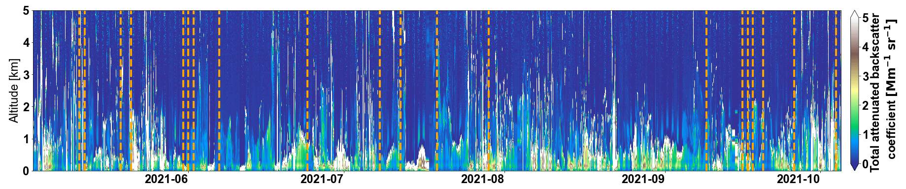
Figure 2 Backscatter coefficient at 1064 nm of CHM 15k ceilometer measurements at the CESAR site from May to November in 2021. The dashed orange lines represent the CAELI measurement availabilities.

2.4 Calculations

The aerosol optical properties (including the scattering coefficient, absorption coefficient, extinction coefficient, backscatter coefficient, and lidar ratio) were calculated based on Mie theory as displayed in Fig. 3a. The main measurement data inputs were (i) chemical composition measured by the ACSM and MAAP as described in Sect. 2.1.1, (ii) PSD measured by the MPSS and APS as described in Sect. 2.1.2, and (iii) RH and temperature profiles obtained from the ECMWF as described in Sect. 2.2.

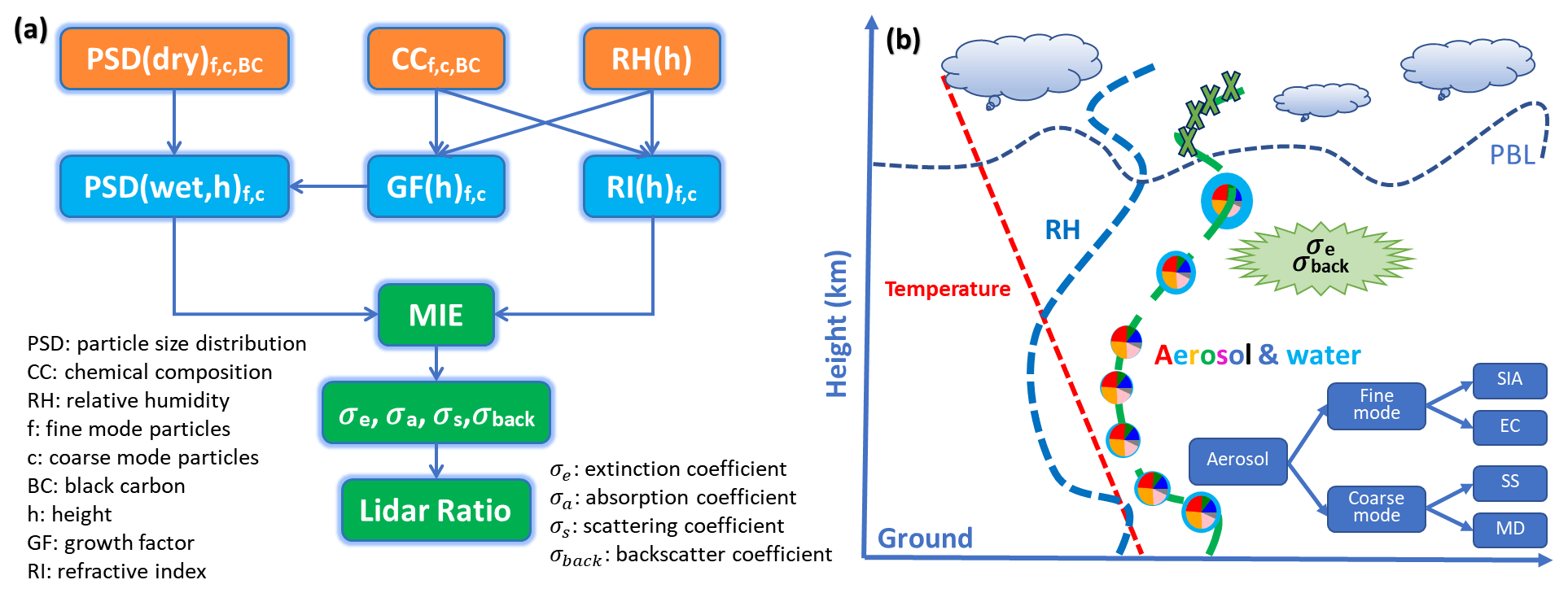
Figure 3 (a) Flow diagram of the calculations used as input for ground-based measurements of particle size distribution (PSD), chemical composition (CC), and vertical profiles of (RH). (b) A sketch of the vertical optical properties' calculations. The abbreviations SIA, BC, SS, and MD refer to secondary inorganic aerosol, black carbon, sea salt, and mineral dust, respectively.

The PSD was derived by combining data from both the MPSS and the APS, as detailed in Sect. S1 in the Supplement. Starting with the dry aerosol, the PSD data were then separated into fine mode (<2.5 µm) and coarse mode (>2.5 µm). We assumed that the fine mode was composed of an internal mixture of secondary inorganic aerosols (SIAs), including ammonium, nitrate, sulfate, and organics, and that BC was externally mixed. The particle size distribution of BC was derived by multiplying its volumetric proportion within PM_2.5 by the overall fine particle size distribution. In addition, we assumed that the coarse mode was composed of sea salt (SS) and mineral dust (MD) (Schaap et al., 2010). Because the coarse-mode chemical composition was not measured during the RITA campaign, we employed the average SS and MD fractions obtained from the previous TROLIX campaign in 2019 (https://ruisdael-observatory.nl/trolix19-tropomi-validation-experiment-2019/, last access: 20 July 2022), which indicated an average composition of 70 % SS and 30 % MD in volume fraction. The densities of SS and MD used are listed in Table 1, and calculation details are in Sect. S3. In addition, we conducted a sensitivity analysis by considering two extreme scenarios: one where the coarse mode was entirely composed of SS and another where it was entirely composed of MD. The outcomes of these sensitivity tests are elaborated upon in the subsequent discussion. A uniform chemical composition was assumed for both fine mode and coarse mode.

Table 1 The refractive index, density, and kappa values of the chemical composition.

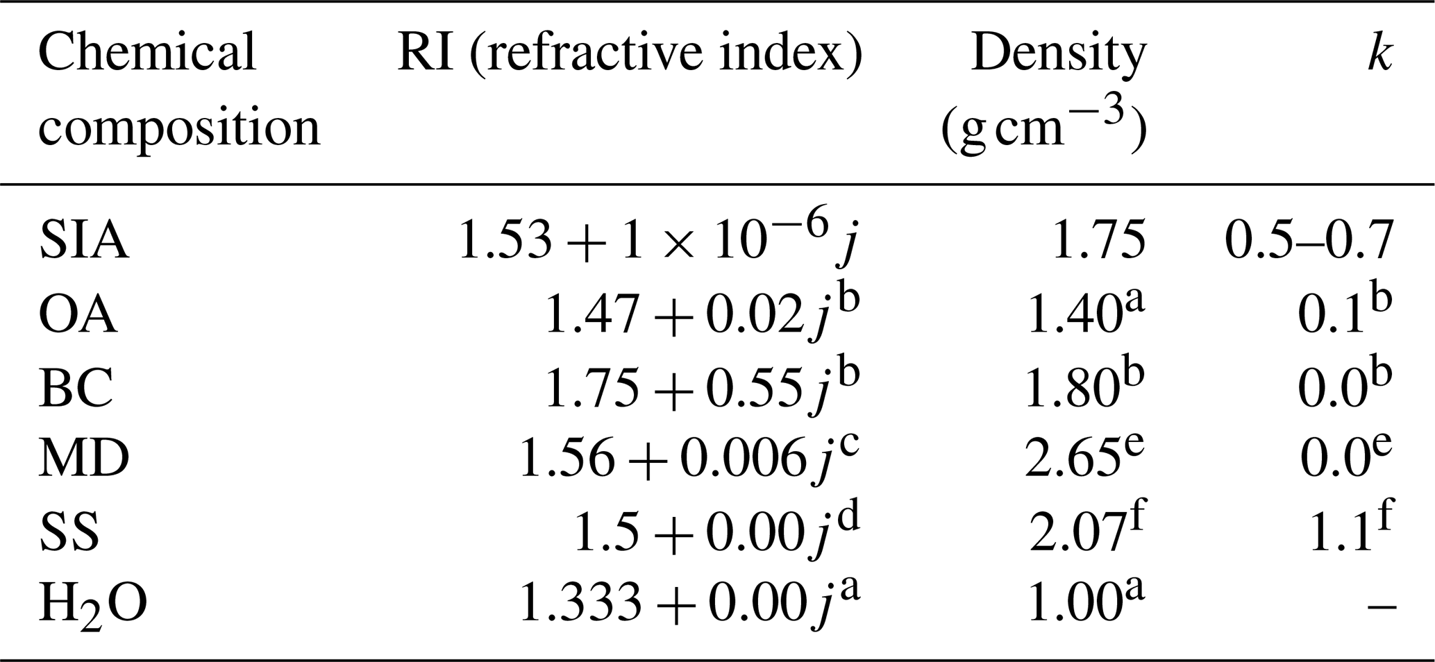
^a Zou et al. (2019). ^b Düsing et al. (2021). ^c Di Biagio et al. (2019). ^d Bi et al. (2018). ^e Di Biagio et al. (2019). ^f Zieger et al. (2017).

The refractive index (RI) of the SIA fine mode and of coarse mode was calculated as a volume-weighted average of the RI of the individual species (RI_s) (as shown in Table 1).

$$\begin{array}{}\text{(1)}& \text{RI}={\sum }_s{\text{RI}}_s{\displaystyle \frac{M_s}{{\mathit{\rho }}_s}},\end{array}$$

where M_s is the mass concentration of species (s) and ρ_s is the corresponding density, shown in Table 1. The RI used for BC is also given in Table 1.

Given the PSDs and the RIs of the dry SIA fine mode, coarse mode, and BC, a Mie model (PyMieSca v1.7.5; Sumlin et al., 2018) was used to calculate the aerosol optical properties, namely the aerosol scattering coefficient, backscatter coefficient, extinction coefficient, and lidar ratio at the wavelengths of the nephelometer. The calculations were compared to the measured scattering coefficient and backscatter coefficient (see in Sect. 3.1). Sensitivity studies show that the calculations of scattering, backscatter, and extinction coefficient are not very sensitive to the assumed BC size distribution.

For the ambient aerosol, a sketch of the calculation for the vertical optical profiles is given in Fig. 3b. In general, we followed the same strategy to separate the aerosol into SIA fine mode and coarse mode and externally mixed BC. A hygroscopic diameter growth factor (GF) was derived for fine mode (only for SIAs because BC was regarded as non-hygroscopic) and coarse mode separately. An ambient PSD was calculated by multiplying the dry particle diameters of fine and coarse mode with a diameter GF derived for the respective RH and temperature as a function of different heights (j) above ground.

$$\begin{array}{}\text{(2)}& {\text{PSD}}_{\text{ambient}}={\text{PSD}}_{\text{dry}}\text{GF}\left(S_j\right),\end{array}$$

where the GF at each altitude j with the given saturation ratio (S_j) is estimated using kappa values (Zhang et al., 2017; Zou et al., 2019; Petters and Kreidenweis, 2013).

$$\begin{array}{}\text{(3)}& \text{GF}\left(S_j\right)={\left({\displaystyle \frac{K_{\text{mix}}{S}_j}{K_{ej}-S_j}}+\mathrm{1}\right)}^{\mathrm{1}/\mathrm{3}}\end{array}$$

with

$$\begin{array}{}\text{(4)}& K_{ej}=\exp \left({\displaystyle \frac{\mathrm{4}\mathit{\sigma }{M}_{\mathrm{w}}}{R{T}_j\mathit{\rho }}}\right),\end{array}$$

where K_mix is the volume-weighted average of the individual kappa values of the compound classes listed in Table 1. For SIAs, upper and lower limits (0.5–0.7) were used and accounted for in the uncertainty of the calculated optical properties. K_ej depends on temperature T, which varies with altitude. σ is the surface tension of the solution–air interface (here we assume σ=0.072 J m⁻²), M_w is the molecular weight of water (M_w=18 g mol⁻¹), R is the universal gas constant (R=8.3145 $\mathrm{J}{\mathrm{mol}}^{-\mathrm{1}}{\mathrm{k}}^{-\mathrm{1}}$), T (K) is temperature, and ρ is the density of water (ρ=1000 kg m⁻³). This results in two externally mixed ambient size distributions for fine mode: black carbon retains the original dry size distribution, and the ambient size distribution of SIAs depends on the RH.

Given the GF at height j, the total water volume concentration can be obtained from the difference between the wet integral particle volume size distribution and the dry integral particle volume size distribution based on the following equation:

$$\begin{array}{}\text{(5)}& V_{{\mathrm{H}}_{\mathrm{2}}\mathrm{O}j}={\sum }_i{\displaystyle \frac{\mathit{\pi }{D}_{\text{dry}i}^{\mathrm{3}}}{\mathrm{6}}}({\text{GF}}_j^{\mathrm{3}}-\mathrm{1})\mathrm{d}{n}_i,\end{array}$$

where the dn_i is the number concentration (cm⁻³) of size bin (i) and D_dry is the corresponding dry particle diameter (nm). The wet RI for coarse and fine mode was calculated as the volume-weighted average of the individual RIs of all chemical constituents, now including the calculated water volume concentration in addition to the original volume concentrations. Finally, the optical properties of the ambient aerosol were calculated based on the Mie model, with ambient RIs and PSDs as input parameters. The vertical profiles of RIs and PSDs were derived by using the corresponding meteorological profile (RH and temperature) with the assumption of a homogenous distribution of the aerosol within the boundary-layer height as sketched in Fig. 3b. The vertical profiles predicted by the model are compared to the Raman lidar measurements in Sect. 3.2.

We quantified uncertainties by assessing a set of nine parallel experimental results. These results were obtained by varying two key parameters as mentioned in the previous content: the volume fraction of SS and MD with values of 1, 0.7, and 0 and the SIA kappa values of 0.5, 0.6, and 0.7. The standard deviation of these parallel results serves to calculate uncertainties.

3 Results and discussion

3.1 Optical properties compared by calculation and nephelometer at ground level

The nephelometer (at 450, 550, and 700 nm) was operated continuously to measure the aerosol scattering coefficient and backscatter coefficient at RH below 40 %. Data from May to the end of October during the RITA-2021 campaign were used to validate the model calculations. Figures 4 and 5 show the time series of the scattering coefficient and backscatter coefficient at three wavelengths obtained by nephelometer measurements and by the calculations outlined in Sect. 2.4. The corresponding scatter plots including best-fit lines are given on the right. Gaps in the calculated data are mainly due to maintenance and power failures of the aerosol in situ instruments, but the data coverage is more than 90 %. Good agreement was found between the measured and calculated scattering coefficients, with a slope of 0.84 (R²=0.90) for 450 nm, 0.95 (R²=0.91) for 550 nm, and 0.96 (R²=0.92) for 700 nm. The model slightly underestimated the measurements, but the difference becomes smaller at larger wavelengths. Good agreement was also found for the backscatter coefficient, with the slope of the calculated values vs. the measured values given as 1.01 (R²=0.67) for 450 nm, 1.18 (R²=0.74) for 550 nm, and 1.12 (R²=0.77) for 700 nm. The model calculations shown in Figs. 4 and 5 assume that the coarse mode is composed of 70 % SS and 30 % MD as described in Sect. 2.4. Results from a sensitivity study assuming that the coarse mode consisted either entirely of SS or entirely of MD are presented in Table S1 in the Supplement, and they are very similar to the results in Figs. 4 and 5. More specifically, under the given particle size distribution conditions, the scattering coefficients for these two extreme scenarios differ by less than 4 % on average across varying wavelengths, and the backscatter coefficients differ by less than 19 %. This shows that the backscatter coefficient is more sensitive to the coarse-mode chemical composition, which can explain the lower R² values in Fig. 5 compared to Fig. 4. However, in general, an average chemical composition of the coarse mode for the site is sufficient to predict the optical properties with reasonable accuracy. This is a considerable advantage, as the coarse-mode chemical composition is usually not as readily available as the fine mode composition for many sites. For sites where the coarse mode comprises a very high mass fraction of PM₁₀, a more accurate representation of the coarse-mode chemical composition might be necessary for predicting the backscatter coefficient.

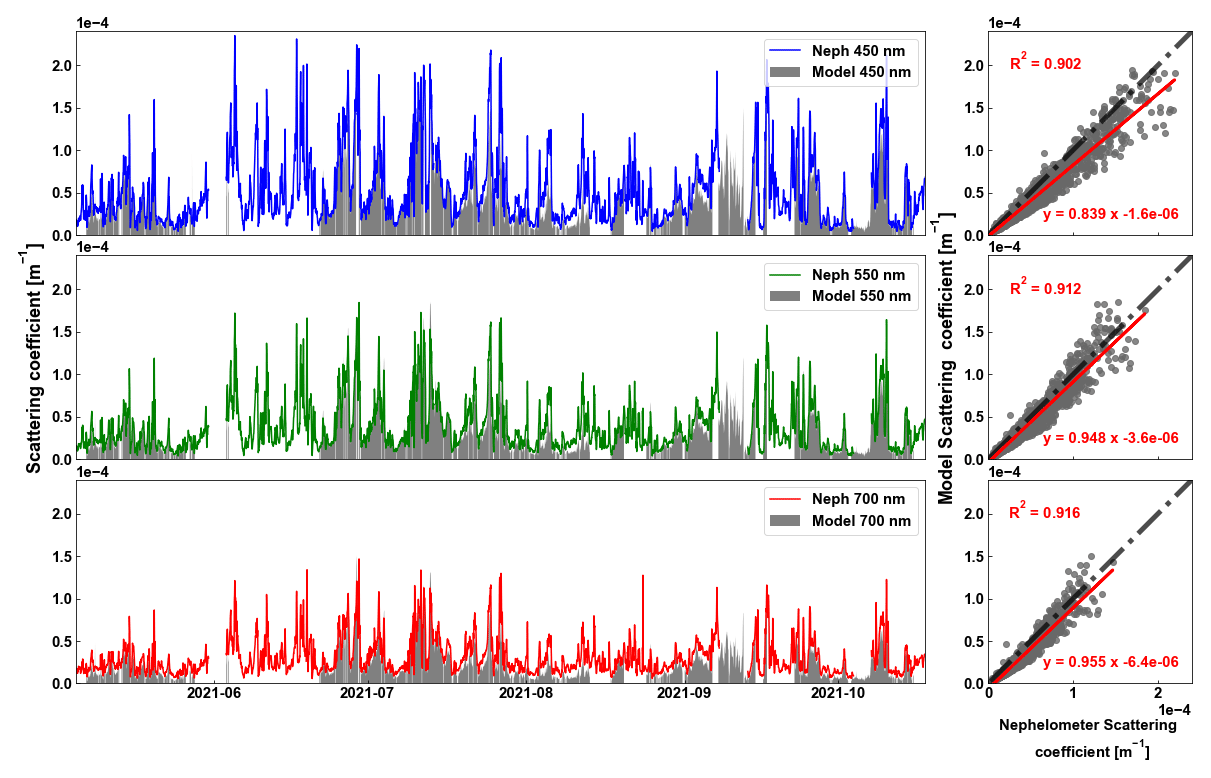
Figure 4 Time series of the scattering coefficient at three wavelengths (450, 550, and 700 nm from top to bottom, respectively) measured by the nephelometer (coloured lines) and calculated from the Mie model (grey shades) in the left panel, along with a scatter plot of each wavelength between the measured scattering coefficient (horizontal axis) and the calculated scattering coefficient (vertical axis) in the right panel. The red line represents the regression line, and the dashed black line represents the 1:1 line.

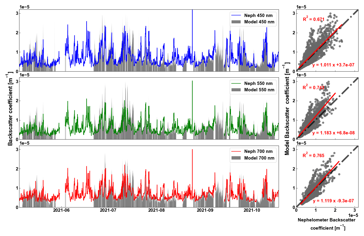
Figure 5 Time series of the backscatter coefficient at three wavelengths (450, 550, and 700 nm from top to bottom, respectively) measured by the nephelometer (coloured lines) and calculated from the Mie model (grey shades) in the left panel, along with a scatter plot of each wavelength between the measured backscatter coefficient (horizontal axis) and the calculated scattering coefficient (vertical axis) in the right panel. The red line represents the regression line, and the dashed black line represents the 1:1 line.

3.2 Comparison between the predicted ambient profiles and Raman lidar retrievals

The time periods when the CAELI Raman lidar was operated are marked in Fig. 2. Due to unsuitable weather conditions, e.g. shallow atmospheric boundary layer or low cloud layers, it was not possible to retrieve lidar profiles for all time periods. Three representative examples, comprising two polluted cases and one clean case, were selected for detailed discussion in the subsequent section. Additional brief discussions on four more cases are provided in the Supplement.

3.2.1 Polluted cases

Figure 6 presents the case from 20:00:21 to 20:53:07 UTC on 19 May 2021. It includes averaged vertical profiles of aerosol optical properties obtained from Raman lidar retrievals and model calculations, 72 h backward trajectories from three altitudes (100, 900, and 1600 m), the high-resolution Raman lidar measurements at 1064 nm, and the chemical composition from ground measurements. To clarify, the specified time period pertains to the lidar data: for the remaining datasets, the closest time range was selected based on their respective temporal resolutions. In particular, the radiosonde, typically launched once daily around midnight, in this instance recorded a vertical profile from 23:30 to 23:46 UTC. Model uncertainties represent the standard deviation across various sensitivity studies, as explained in Sect. 2.4. The ECMWF profiles show an uncertainty of 10 %. In addition, the valid lidar measurement levels are marked in the green background in Fig. 6. The lowest altitude for the backscatter coefficient is above 150 m, whereas the lowest altitude for the extinction coefficient and lidar ratio is 810 m, as described in Sect. 2.3.1. Furthermore, the upper limits were manually selected to only include aerosols originating from the planetary boundary layer (PBL; including the residual layer, if present) for all the profiles, excluding lofted layers possibly originating from long-range transport. All the subsequent profiles adhered to the same approach. In this case, the dataset spanning from 810 to 2370 m was employed for subsequent lidar ratio calculations and for comparison to the model calculations.

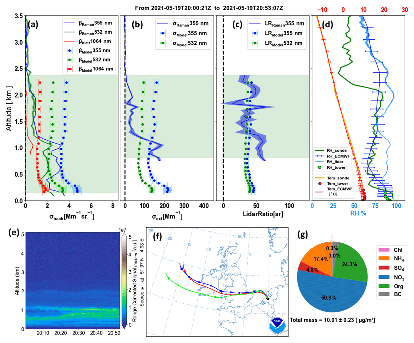
Figure 6 Vertical profiles of the aerosol optical properties. (a) The Raman lidar backscatter coefficients (σ_back) at 355 nm (blue line), 532 nm (green line), and 1064 nm (using the Klett method; red line). The uncertainties of the measurements are given by the shaded areas. The backscatter coefficient predicted by the Mie calculations at 355 nm (blue dots), 532 nm (green dots), and 1064 nm (red dots), with error bars representing the corresponding uncertainties. (b) The extinction coefficient (σ_ext) profiles of the lidar measurements and predictions. (c) The corresponding lidar measured and the calculated lidar ratio profiles. The light-green background represents the upper and lower limits of the valid lidar measurements in panels (a)–(c). (d) The vertical profiles of the RH% and temperature from the ECMWF, from the Raman lidar, from the tower in situ (between 20:00 and 21:00), and from the radiosonde (launched from 23:30 to 23:46). (e) The 72 h back trajectories at 100 m (in red), 900 m (in blue), and 1600 m (in green) from 20:00 to 21:00. (f) The CAELI Raman lidar range-corrected signal (RSC) at 1064 nm from 20:00 to 20:53. (g) Mass fractions of the chemical composition from 20:00 to 21:00. All times listed are UTC on 19 May 2021.

For this study case, the Raman lidar image (Fig. 6e) shows that, at altitudes below approximately 1000 m, aerosols exhibit layers, but they are not distinctly pronounced. Therefore, the lidar-retrieved backscatter coefficients (Fig. 6a) exhibit slight fluctuations in the vertical direction. Between altitudes of 600 and 1100 m, the retrieved and calculated backscatter coefficients agreed within 12 %. Specifically, within this range, the lidar reports values of 2.9 ${\mathrm{Mm}}^{-\mathrm{1}}{\mathrm{sr}}^{-\mathrm{1}}$ for 355 nm and 2.0 ${\mathrm{Mm}}^{-\mathrm{1}}{\mathrm{sr}}^{-\mathrm{1}}$ for 532 nm, comparable with calculated values of 3.3 ${\mathrm{Mm}}^{-\mathrm{1}}{\mathrm{sr}}^{-\mathrm{1}}$ for 355 nm and 2.1 ${\mathrm{Mm}}^{-\mathrm{1}}{\mathrm{sr}}^{-\mathrm{1}}$ for 532 nm. Below 500 m, the simulated values are higher than the measured values, which is probably partially due to higher values in RH of the ECMWF data compared to the radiosonde measurements in Fig. 6d but potentially also due to the formation of a stable layer near the ground, as shown by an increase in temperature with height in the tower data. Beyond 1100 m, the measured backscatter coefficients rapidly decrease to nearly 0 above the mixed layer and the comparison with ground-based data ceases to be meaningful. This case study demonstrates that ground-based measurements are not very well suited for estimating vertical profiles of extensive aerosol properties (such as the scattering coefficient) under conditions with poor mixing, which often occur during evening and nighttime.

For the extinction coefficient profiles (Fig. 6b), the Raman lidar retrievals provided good-quality data only for 355 nm. A limited overlap existed between the valid lowest retrieved level and the aerosol layer at 1000 m, posing challenges for direct comparisons. The average extinction coefficient at 355 nm, ranging from 800 to 1200 m, is approximately 130 Mm⁻¹ for calculations and slightly higher for retrievals at about 145 Mm⁻¹.

Finally, the retrieved lidar ratio is 45.1 ± 13.7 sr⁻¹ at 355 nm for the valid altitudes, whereas the calculations yield a lidar ratio of 40.1 ± 1.6 sr⁻¹ at 355 nm and 35.3 ± 1.4 sr⁻¹ at 532 nm, as shown in Fig. 6c, showing relatively good agreement between calculations and retrievals. This range of values is typical for a polluted aerosol type (Bohlmann et al., 2018; Groß et al., 2013; Illingworth et al., 2015). The 72 h back-trajectory analysis (Fig. 6f) at three different altitudes using the HYSPLIT model (Stein et al., 2015; Rolph et al., 2017) implies that the air masses originated from the sea but were transported over Ireland and the United Kingdom and also the northwest of the Netherlands, resulting in elevated levels of anthropogenic pollutants. This result is in line with ACSM measurements (shown in Fig. 6g), which indicate an average non-refractory PM_2.5 mass concentration of 10.01 ± 0.23 µg m⁻³. Notably, nitrate (50.9 %) and ammonium (17.4 %) contribute significantly to this mass concentration, which may reflect the substantial contributions from local nitrogen oxides and ammonia emissions to pollution in the Netherlands (Aan de Brugh, 2013).

Figure 7 shows the second case from 21:09:25 to 21:44:35 UTC on 9 September 2021. The valid retrieval range is from 810 to 2430 m. The Raman lidar images displayed in Fig. 7f show complex and variable cloud structures before and after this period. The profiles of backscatter coefficients (Fig. 7a) obtained from Raman lidar retrievals and calculations agree remarkably well from the surface up to an altitude of 1000 m within the mixed-layer height. On average, the differences between the two datasets are less than 5 % for both 355 and 532 nm. Additionally, the backscatter coefficient profiles increased from the surface to 1000 m, from 3.9 to 6.5 ${\mathrm{Mm}}^{-\mathrm{1}}{\mathrm{Sr}}^{-\mathrm{1}}$ for 355 nm and from 2.7 to 4.7 ${\mathrm{Mm}}^{-\mathrm{1}}{\mathrm{Sr}}^{-\mathrm{1}}$ for 532 nm. This increase is reflected in all the RH profiles (from 75 % to 90 % as displayed in Fig. 7d), including those from the ECMWF, Raman lidar, tower, and radiosonde (2.5 h later), which exhibit good consistency. The variations in aerosol optical properties within 1 km altitude were thus primarily due to changes in RH and could be well predicted by ground-based data. However, the ground-based aerosol information is no longer applicable to profiles situated above 1 km.

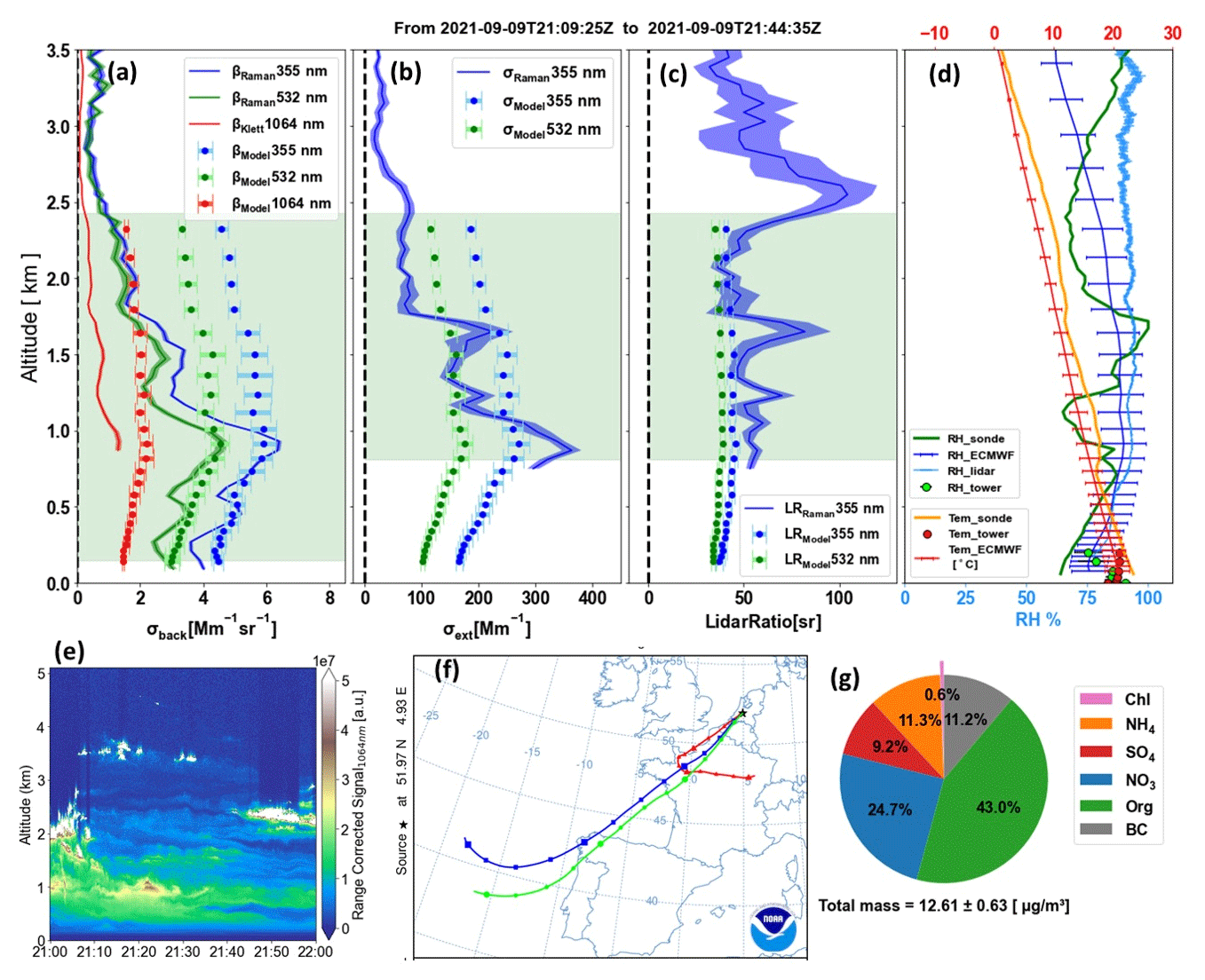
Figure 7 Corresponding to Fig. 6 for the period from 21:09:25 to 21:44:35 UTC on 9 September 2021.

The extinction coefficient profiles (Fig. 7b) initially exhibit higher values at around 850 m, followed by a rapid decrease up to an altitude of approximately 1.2 km. The calculated extinction coefficient also decreases above 850 m but much less. This most likely results from a lower aerosol concentration above the mixed layer, particularly during the latter part of the observation period, as shown in Fig. 7e. Those changes affect the average outcomes of lidar retrievals, resulting in lower values in the extinction profiles. Nevertheless, the extinction profiles of the measurements and calculations at 355 nm agreed reasonably well with a height of about 1 km. Finally, the retrieved and calculated lidar ratios (Fig. 7c) are in good agreement throughout the effective column range except at around 1.5 km, indicating the presence of similar aerosol types. The lidar average retrievals over the valid retrieval height yielded a value of 53.1 ± 10.8 sr⁻¹, while the model calculations produced a value of 43.2 ± 1.7 sr⁻¹ at 355 nm. The analysis of 100 m back trajectories, as depicted in Fig. 7f, demonstrated that the air masses originated from central Europe, while air masses at higher altitudes (900 and 1600 m) are shown to originate from the North Atlantic Ocean, and only the last day of the trajectories is very similar for all altitudes. Optical profiles based on ground-level data prove to be effective for altitudes below 900 m. Compared to the previous polluted case, the ACSM measurements showed a slightly higher PM_2.5 mass concentration of 12.61 ± 0.63 µg m⁻³, as illustrated in Fig. 7g. The main difference lies in the dominant contribution of organic components (43 %).

3.2.2 Clean cases

Figure 8 shows the profiles for the period from 20:00:05 to 21:02:45 UTC on 29 July 2021. The lidar image (Fig. 8e) reveals two aerosol layers (below 1 km and 1–2 km) during this period, and the applicable range for the extinction profile and lidar ratio spans from 810 to 2010 m. Figure 8a shows that the retrieved backscatter coefficient decreases with altitude, but the calculated backscatter coefficient is rather constant with altitude. The calculations underestimate the retrievals at altitudes below 500 m and overestimate the retrievals (by approximately 20 %–30 %) at altitudes around 1500 m. This difference can be attributed to (i) variations in aerosol concentrations or chemical properties between ground-level and higher altitudes and (ii) other inaccuracies in the model, such as insufficient information on the size-resolved chemical composition and aerosol mixing state. (iii) The RH profiles may be inaccurate, where the 1 h time resolution of the re-analysis data does not correctly capture the development of a nocturnal stable layer near the ground. As shown in Fig. 8d, below 200 m, the RH values from the ECMWF and the ground-based tower show good overlap. However, between 200 and 500 m, the RH values calculated by the lidar differ from those of the ECMWF by up to 10 % RH. Due to the absence of direct measurement data (radiosonde data were unavailable on this day), it is challenging to ascertain which dataset is closer to the actual values. (iv) The lidar retrievals near the ground could also be inaccurate, especially at the low aerosol concentrations in this clean case. However, despite these discrepancies, the calculated values are on the order of magnitude of the retrievals and agree within uncertainties for a large part of the profile.

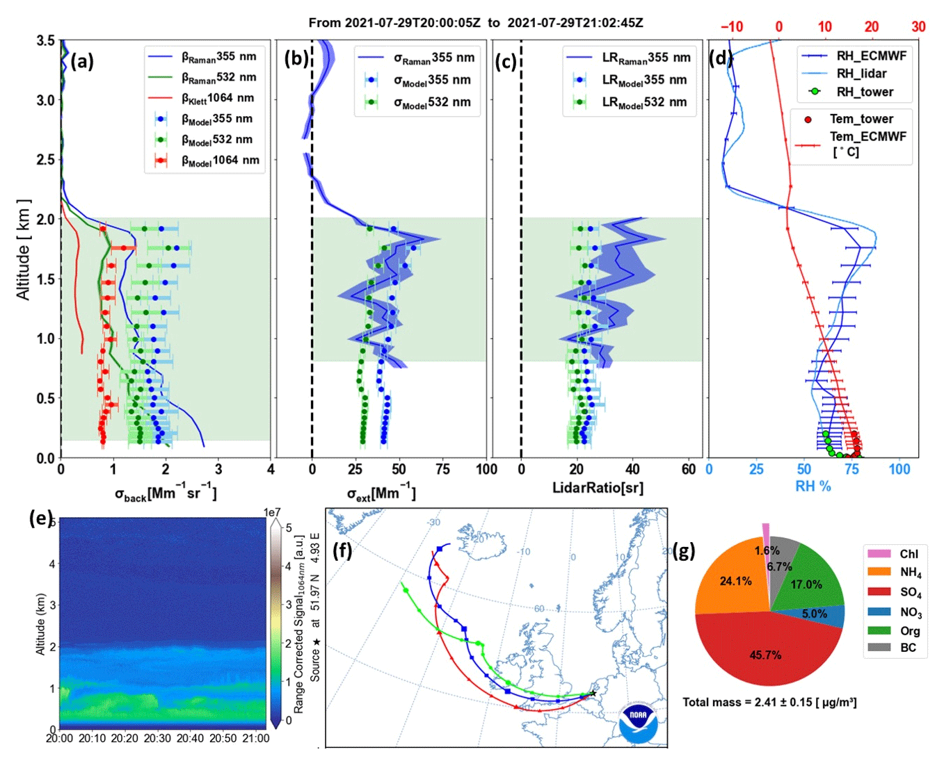
Figure 8 Corresponding to Fig. 6 for the period from 20:00:05 to 21:02:45 UTC on 29 July 2021.

It is noticeable that the calculated backscatter values have larger uncertainties in this clean case than in the polluted cases. The main reason is that, in the clean case, the contribution of the coarse mode to the backscatter coefficient is larger; thus the extreme assumptions regarding the chemical composition (pure sea salt vs. pure mineral dust) start to affect the results. Since sea salt has a much higher growth factor than mineral dust, the ambient size distribution of the coarse mode differs considerably, especially at high RH. Nevertheless, the resulting uncertainties of the backscatter coefficient are still in a reasonable range.

The agreement between the modelled and retrieved values of extinction coefficient (Fig. 8b) and lidar ratio profiles (Fig. 8c) within the altitude range of 800 to 1800 m suggests a reasonable representation of aerosol properties by the ground-based measurements throughout the boundary layer. In particular, the lidar ratio obtained from the Raman lidar measurements at 355 nm was 31.8 ± 6.8 sr⁻¹, while the model-estimated values were 25.0 ± 1.3 sr⁻¹ at 355 nm and 21.5 ± 1.1 sr⁻¹ at 532 nm. These lidar ratios are typical for marine aerosols (around 5 to 30 sr⁻¹) (Bohlmann et al., 2018; Illingworth et al., 2015; Groß et al., 2013). Results are consistent with aerosols originating from marine sources during the observed period, which is supported by the back trajectory shown in Fig. 8f. Additionally, the low aerosol mass concentration (2.41 ± 0.51 µg m⁻³) shown in Fig. 8g with a significantly higher fraction of sulfate (45.7 %) further supports this result.

All remaining profiles marked in Fig. 2 have been stored in a publicly accessible repository (https://doi.org/10.5281/zenodo.11174465; Liu, 2024), available for interested readers. The results show that extinction and backscatter coefficients are sometimes considerably under- or overestimated by the ground-based calculations. However, it is worth emphasising that the lidar ratios are much better predicted. We speculate that the main reasons for this phenomenon are as follows: (i) the upper-level aerosols may have similar chemical composition and size distribution to surface-level aerosols but are present at different concentrations. Thus, the backscatter or extinction coefficients of aerosols may be overestimated or underestimated by the same factor, resulting in a similar lidar ratio. (ii) Alternatively, the meteorological data may not be sufficiently accurate. This has a more significant influence on extinction and backscatter coefficients, especially when the RH is overestimated or underestimated, but its impact on the lidar ratio is less pronounced. (iii) Another crucial factor may be the influence of shape effects, which normally become more significant for the larger particles. Previous studies show that the backscatter cross-section and the extinction cross-section may be underestimated or overestimated by a factor ranging from −2 to +5, depending on the particle shapes and size ranges (Potenza et al., 2016; Geisinger et al., 2017).

3.3 Summary of the lidar ratio comparison

Figure 9a shows the time series of the average lidar ratios (at 355 and 532 nm) for each period retrieved from lidar measurements and calculated by the model for the corresponding valid retrieval levels of each profile. The error bars correspond to the standard deviation of each effective lidar ratio profile. For the most part, the predicted lidar ratios are comparable to the lidar ratios measured by Raman lidar; however, for retrieved lidar ratios above 50 sr, the predictions seem systematically lower. Significant standard deviations in Fig. 9a illustrate that the measured lidar ratios were quite variable across the planetary boundary layer, which might indicate different aerosol layers at various altitudes. This cannot be taken into account for the calculations. Consequently, the model-generated lidar ratios tend to remain relatively stable with altitude for the majority of cases. Nevertheless, the predicted lidar ratios are within the range of retrieved lidar ratios, with differences from case to case usually being smaller than ±30 % for the wavelength at 355 nm as shown in Fig. 9b. On the whole, the calculated lidar ratios were in the range of 16–43 sr at 355 nm and 18–41 sr at 532 nm on average, indicating a relatively low-pollution environment. Furthermore, the calculations show that the lidar ratio has a small wavelength dependence, with a higher lidar ratio on average at 355 nm (slope of 0.64 and R² of 0.94 between the lidar ratio at 355 and 532 nm). This is consistent with findings from Mattis et al. (2004), which summarised long-term Raman lidar measurements with the lidar ratio from 2000 to 2003 for central European haze, specifically the anthropogenic aerosol particles, with values of 58 ± 12 sr for 355 nm, 53 ± 11 sr for 532 nm, and 45 ± 15 sr for 1064 nm wavelengths in the upper part of the PBL. In the free tropospheric and stratospheric layers, the lidar ratio possibly has a different wavelength dependence, where Haarig et al. (2018) reported that the lidar ratios were 40–45 sr for 355 nm, 65–80 sr for 532 nm, and 80–95 sr for 1064 nm.

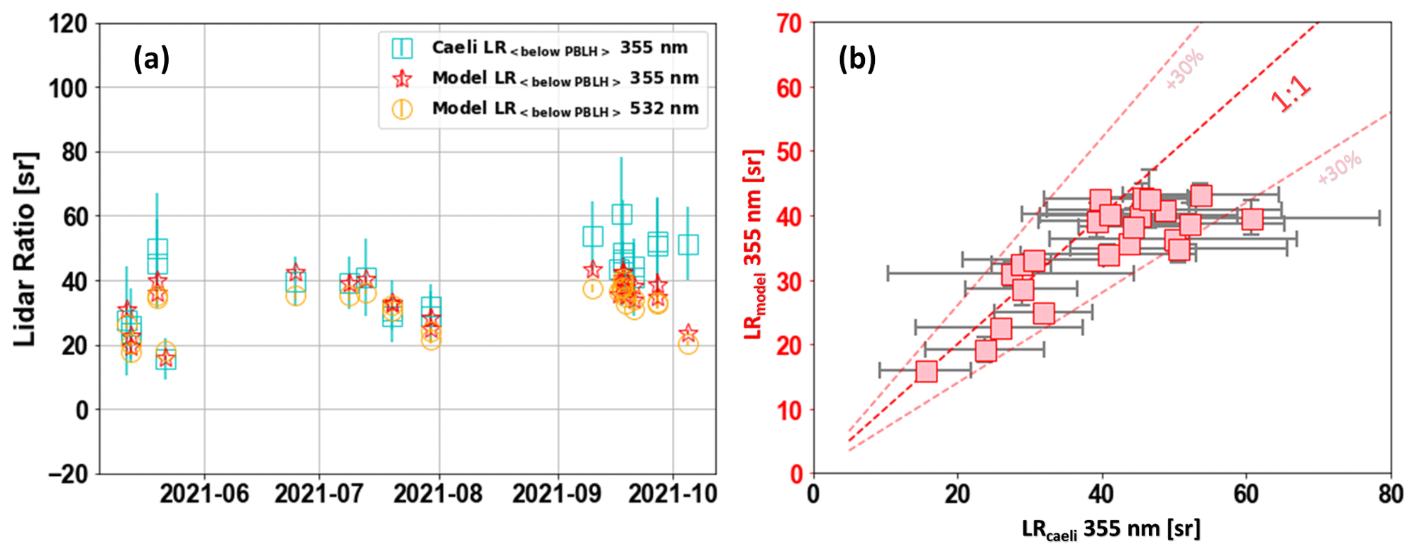
Figure 9 (a) Time series of the mean lidar ratio and its uncertainty (at 355 and 532 nm) from the valid lidar retrievals and the calculations. (b) Scatter plot of the lidar ratios (LRs) from Raman lidar measurements (x axis) and from calculations (y axis) at 355 nm.

In summary, by integrating data from in situ measurements with the readily accessible ECMWF data, we can predict aerosol optical properties to a certain extent when the aerosol mixing is homogeneous below the boundary layer. Such conditions are more likely during the day but occur less often during the evening and night, when Raman lidar data are typically available. While not as sensitive as the retrievals, the calculations are capable of capturing significant shape changes in the vertical distribution. Despite occasional overestimations and underestimations of backscatter and extinction values when assumptions deviate from actual conditions (i.e. homogeneous aerosol mixing), our predictions for the lidar ratio are very effective up to heights of about 2 km. This would allow the estimation of lidar ratios applicable to simple backscatter lidars from ground-based in situ measurements. For such calculations, it is crucial for the model to be furnished with an accurately measured particle size distribution including the coarse mode. Therefore, if the sampling site contains a higher concentration of coarse-mode particles, particularly those larger than 10 µm, the particle loss effects during the sampling process by the in situ measurements could potentially become significant. While possessing chemical insights into the coarse mode is an advantage, it is not absolutely necessary, as long as a typical composition can be assumed. In our case studies, we showed that the extreme assumptions of pure sea salt aerosols vs pure mineral dust aerosols for the coarse mode resulted in reasonable uncertainties in the predicted optical properties for coarse-mode mass fractions about 49 % on average (range from 14 %–81 %). This, however, does not take into account the uncertainties regarding the shape of pure mineral dust aerosols, which could be considerable. Therefore, in regions dominated by dust aerosols, the simple assumption of spherical particle shape might not be appropriate and could result in much larger bias. Within the mixed layer, our results show that the enhancement of the backscatter coefficient and extinction coefficient strongly depends on the particle hygroscopic growth. Consequently, the availability of an accurate and high-vertical-resolution RH profile is important for constructing a robust model input, but even 1-hourly ECMWF humidity fields give reasonable results.

4 Conclusions

In this study, a Mie theory-based model was applied to ground-based in situ measurements to predict ambient aerosol optical properties, including scattering coefficient, backscatter coefficient, extinction coefficient, and lidar ratio. The input data are (i) aerosol chemical composition and (ii) particle size distribution measured at the surface and (iii) meteorological data from the European Centre for Medium-Range Weather Forecasts (ECMWF). The data were collected during the Ruisdael Land–Atmosphere Interactions Intensive Trace-gas and Aerosol (RITA) campaign at the CESAR site in the Netherlands with a total time span of 5 months (from May to October in 2021). The calculations were first validated by comparison to observations from the TSI integrating nephelometer at dry conditions for the entire period. The calculations and measurements took place across multiple wavelengths, with slopes of 0.84–0.96 (R²≥0.90) for the scattering coefficients and slopes of 1.01–1.18 (R²≥0.67) for the backscatter coefficients. Furthermore, the model was compared with aerosol optical vertical profiles retrieved by a multi-wavelength Raman lidar. The results showed that, for a homogeneously distributed aerosol within the mixing layer, the model could effectively simulate the vertical profile of the aerosol backscatter coefficient as a function of RH, which varies with altitude. The comparison of extinction coefficients posed challenges due to the limited overlap between the lower layer of retrievals and the mixed layer. However, the profiles at the shared levels exhibited a reasonable connection, suggesting a meaningful comparison could still be made. The simulated lidar ratio can predict the measured lidar ratio within ±30 % for the average values below the height of the planetary boundary layer. In summary, our research demonstrates that a full measurement of particle size distribution, encompassing both fine and coarse particle modes, along with chemical composition and relative humidity, are crucial inputs for the model to generate accurate backscatter and extinction coefficient profiles. Nevertheless, in the well-mixed boundary layer, it is usually possible to approximate the lidar ratio using ground-based measurements. This approach allows the extension of extinction profiles to lower altitudes that are typically challenging to retrieve, or it can be employed alongside basic backscatter lidar systems to calculate the extinction and then the aerosol optical depth, which could potentially extend to forecasting aerosol optical depth and could offer advantages in extensive-scale or worldwide radiation simulations.