the Creative Commons Attribution 4.0 License.
the Creative Commons Attribution 4.0 License.
 | 22 Aug 2024
Exploring aerosol–cloud interactions in liquid-phase clouds over eastern China and its adjacent ocean using the WRF-Chem–SBM model
Jianqi Zhao
Johannes Quaas
Hailing Jia
In this study we explore aerosol–cloud interactions in liquid-phase clouds over eastern China (EC) and its adjacent ocean (ECO) using the WRF-Chem–SBM model with four-dimensional assimilation. The results show that our simulations and analyses based on each vertical layer provide a more detailed representation of the aerosol–cloud relationship compared to the column-based analyses which have been widely conducted previously. For aerosol activation, cloud droplet number concentration (Nd) generally increases with aerosol number concentration (Naero) at low Naero and decreases with Naero at high Naero. The main difference between EC and ECO is that Nd increases faster in ECO than EC at low Naero due to abundant water vapor, whereas at high Naero, when aerosol activation in ECO is suppressed, Nd in EC shows significant fluctuation due to strong surface effects (longwave radiation cooling and terrain uplift) and intense updrafts. Cloud liquid water content (CLWC) increases with Nd, but the increase rate gradually slows down for precipitating clouds, while CLWC increases and then decreases in non-precipitating clouds. Higher Nd and CLWC can be found in EC than in ECO, and the transition-point Nd value at which CLWC in non-precipitating clouds changes from increasing to decreasing is also higher in EC. Aerosol activation is strongest at moderate Naero, but CLWC increases relatively fast at low Naero. ECO cloud processes are more limited by cooling and humidification, whereas strong and diverse surface and atmospheric processes in EC allow intense cloud processes to occur under significant warming or drying conditions.
- Article
(14385 KB) - Full-text XML
-
Supplement
(1676 KB) - BibTeX
- EndNote


Atmospheric aerosols have significant effects on the Earth's radiation balance, water cycle, and climate system through direct absorption and scattering of solar radiation, and they also have indirect effects on cloud formation and development by acting as cloud condensation nuclei (CCN) and ice nuclei (IN) (Carslaw et al., 2010; Wilcox et al., 2013; Tian et al., 2021). The latter, known as the aerosol indirect effect, or more recently defined by the Intergovernmental Panel on Climate Change (2013) as effective radiative forcing due to aerosol–cloud interactions (RFaci), remains a challenging scientific topic in climate assessment and prediction because of its complex mechanisms and high uncertainties (Church et al., 2013; Jia et al., 2019a; Arias et al., 2021). Liquid-phase clouds offer great opportunities to untangle the aerosol indirect effect due to their sheer abundance and impact on cloud radiative forcing (Christensen et al., 2016).
Twomey (1977) pointed out that, under a constant cloud water content, the activation of atmospheric aerosol particles entering into clouds leads to an increase in cloud droplet number concentration (Nd), a decrease in droplet size, and an increase in cloud albedo. This mechanism, termed the aerosol first indirect effect, is revealed to be the key driver of the aerosol indirect effect; besides, the rapid adjustments also contribute significantly (Quaas et al., 2020). Two key competing mechanisms exist in the latter, one of which is that an increase in Nd causes a decrease in precipitation efficiency and, with this, a co-increase in cloud liquid water path (CLWP) and cloud fraction (CF). This mechanism dominates in precipitation clouds (Albrecht, 1989). The other mechanism dominates in non-precipitating clouds; i.e., with limited water content, the decrease in droplet size reduces sedimentation velocity and increases cloud-top liquid water content, resulting in additional cloud-top cooling and pushing further entrainment and evaporation (Bretherton et al., 2007). Moreover, as cloud droplets decrease in size, their ratio of surface area to volume is higher and evaporation is faster, resulting in further enhancement of the negative buoyancy at cloud top (Small et al., 2009). Numerous studies have been conducted to assess the contribution of these three mechanisms. Statistical analysis based on satellite-retrieved data indicates that the CLWP of marine low clouds exhibits a weak decreasing trend with rising Nd caused by aerosol increase (Michibata et al., 2016; Rosenfeld et al., 2019). Gryspeerdt et al. (2019) found that CLWP is positively correlated with Nd at low Nd and droplet size greater than the precipitation threshold; i.e., delayed precipitation leads to increased CLWP. In contrast, for the clouds with high Nd and a low possibility of precipitation, CLWP shows a negative correlation with Nd. In this case, the increase in aerosol leads to the decrease in cloud droplet size and the increase in Nd, which in turn accelerates the mixing and evaporation process and makes CLWP decrease. The CLWP response to aerosols differs clearly between precipitation and non-precipitating clouds because of the significant influence of the precipitation process on CLWP (Christensen and Stephens, 2012). CLWP has a significant positive correlation with the aerosol index (AI) in precipitation clouds and the opposite in non-precipitating clouds (Chen et al., 2014). Furthermore, the response of CLWP to aerosols highly depends on meteorological conditions. Chen et al. (2014) indicated that CLWP and aerosol concentration show a negative correlation when entrainment mixing exerts a marked impact on the cloud-side evaporation process (which usually occurs under free troposphere with dry and unstable atmosphere), and this relationship shifts to positive as the atmosphere becomes moist and stable. Such statistical analysis, however, suffers severely from retrieval uncertainties (Arola et al., 2022). In turn, “opportunistic experiments”, such as the analysis of ship and pollution tracks, also hint at a decrease in CLWP but an increase in cloud horizontal extent in response to aerosol increases (Toll et al., 2019; Christensen et al., 2022). In spite of considerable efforts in recent research to unravel aerosol–cloud interactions, it remains challenging to distinguish and quantify underlying mechanisms of aerosol–cloud interactions under diverse air pollution and meteorological conditions.
In order to further resolve the mechanisms of aerosol–cloud interactions, the proper use of numerical simulations is necessary. Current global climate models (GCMs) have difficulties in accurately representing the response of clouds to aerosols, which is mainly due to (1) the limitation of coarse model resolution, (2) the absence of sufficient consideration of cloud droplet spectral characteristics, and (3) the fact that most current GCMs parameterize the precipitation mechanism through the autoconversion process as an inverse function of Nd without accurate representation of entrainment–mixing processes (Quaas et al., 2009; Bangert et al., 2011; Michibata et al., 2016; Zhou and Penner, 2017). Regional climate models (RCMs) with higher resolution and finer physical parameterization can effectively compensate for at least some of these shortcomings and better reproduce the physical processes, which help to further distinguish and quantify the aerosol–cloud interaction mechanisms (Li et al., 2008; Bao et al., 2015). The Weather Research and Forecasting (WRF) model has been widely used in regional numerical simulation studies because of its advanced technology in numerical calculation, model framework, and program optimization, which has many advantages in portability, maintenance, expandability, and efficiency (Maussion et al., 2011; Islam et al., 2015; Xu et al., 2021). The chemistry-coupled version of the WRF model (WRF-Chem) allows us to simulate the spatial and temporal distributions of reactive gases and aerosols, spatial transport, and their interconversion while simulating meteorological fields and atmospheric physical processes (Tuccella et al., 2012; Sicard et al., 2021). Bulk and bin approaches are commonly utilized to simulate regional cloud microphysical processes. Bulk schemes diagnose the size distribution of hydrometeors based on different predicted bulk mass (one-moment schemes) or number- and mass mixing ratios (double-moment schemes) and assumed size distribution, showing significant limitations in reproducing processes such as condensation, deposition, and evaporation (Lebo et al., 2012; Wang et al., 2013; Fan et al., 2015). Bin schemes predict the size distribution of hydrometeors based on a number of discrete bins, enabling better representation of cloud microphysical processes. As stated by Khain et al. (2015), previous studies have demonstrated that bin schemes outperform bulk schemes in simulations. The evaluation of WRF-Chem cloud microphysics by Zhang et al. (2021a) also showed that the bin scheme using the explicit approach reproduced the aerosol-induced convection and precipitation enhancement that the bulk scheme using the saturation-adjusted approach failed to model. In this study, the WRF-Chem–SBM model (Gao et al., 2016) is used, in which the Model for Simulating Aerosol Interactions and Chemistry (MOSAIC) in WRF-Chem (Fast et al., 2006) is coupled with a spectral-bin microphysics (SBM) scheme (Khain et al., 2004). In WRF-Chem–SBM, aerosol information is provided for cloud microphysical simulations, and cloud microphysical parameters are offered to aerosol chemistry simulations, which are of great help in reproducing accurate aerosol and cloud conditions and in distinguishing and quantifying aerosol–cloud interaction mechanisms.
Eastern China (EC) is one of the most human-active regions worldwide, resulting in numerous anthropogenic aerosol emissions. The contrast between the high-aerosol-content air masses of EC and the relatively clean air masses of the Pacific Ocean makes EC and its adjacent ocean (ECO) ideal regions for exploring aerosol–cloud interactions (Fan et al., 2012; Wang et al., 2015; Zhang et al., 2021b). It is shown that low clouds contribute the most to the Earth's energy balance due to their broad coverage and the albedo effect governing their impact on emitted thermal radiation (Hartmann et al., 1992). The statistics of Niu et al. (2022) using the satellite data from 2007–2016 show that low clouds in EC and ECO occur most frequently in winter, reaching more than 50 %, with stratocumulus clouds, which are persistent and sensitive to aerosol variations (Jia et al., 2019b), constituting more than 70 % of the low clouds. Therefore, the EC and ECO aerosol–cloud response in winter is an ideal condition to investigate aerosol–cloud interactions in liquid-phase clouds. Based on the WRF-Chem–SBM model, we investigate the aerosol–cloud interaction mechanisms of EC and ECO in winter by obtaining detailed and high-resolution aerosol and cloud parameters along with meteorological information through the reproduction of real scenarios.
The paper is structured as follows: Sect. 2 introduces the model configuration and observational data used in the study, Sect. 3 presents the evaluation of simulated results and the analysis of aerosol–cloud responses presented in the simulations, and the summary is given in Sect. 4.
2.1 Simulation setup
We performed model simulations using the WRF-Chem–SBM (Gao et al., 2016), in which the four-bin MOSAIC aerosol module treats the mass and number of nine major aerosol species, including sulfate, nitrate, sodium, chloride, ammonium, black carbon, primary organics, other inorganics, and liquid water (Zaveri et al., 2008). The diameters of the four bins are 0.039–0.156, 0.156–0.624, 0.624–2.5, and 2.5–10.0 µm, respectively, and aerosol particles are assumed to be internally mixed. This module is capable of treating processes such as emissions, new particle formation, particle growth/shrinkage due to uptake/loss of trace gases, coagulation, and dry and wet deposition (Sha et al., 2019). In addition, this model incorporates the fast version of SBM, which solves a system of prognostic equations for three hydrometeor types (liquid drops, ice/snow, and graupel) and CCN size distribution functions (Khain et al., 2010). Each size distribution is structured by 33 mass-doubling bins (i.e., the mass of the particle in the kth bin is twice that of the k−1th bin). The cloud microphysical processes described in SBM contain aerosol activation, freezing, melting, diffusion growth/evaporation of liquid drops, deposition/sublimation of ice particles, and drop and ice collisions.
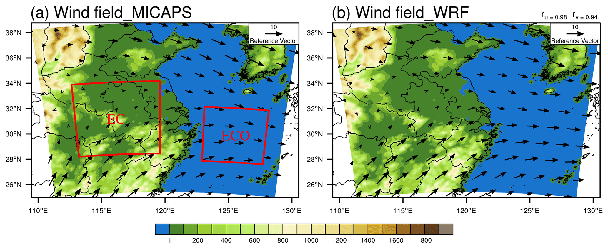
Figure 1Topography (unit: m) of the model domain, MICAPS (a), and assimilated simulated (b) 850 hPa wind fields (unit: m s−1) during the simulation period, with their correlation coefficients of u and v components (ru, rv) given in the upper-right corner.
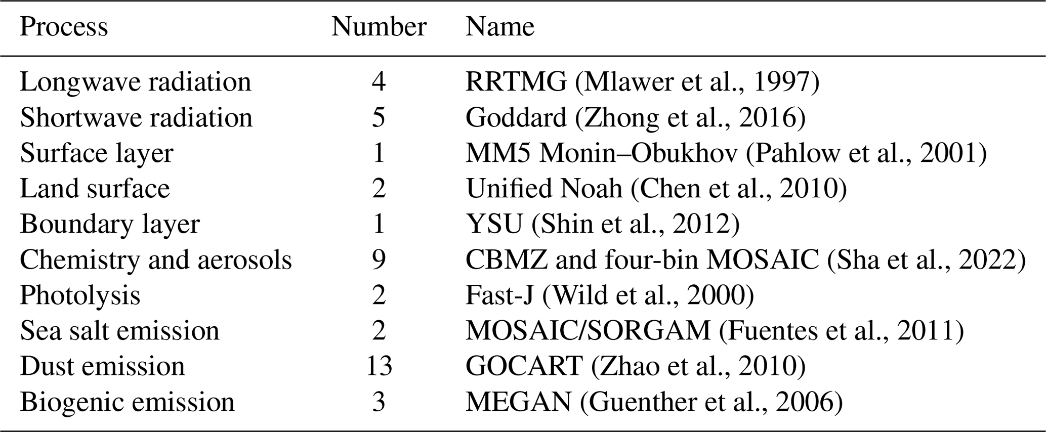
The model domain is shown in Fig. 1, and two-layer nested grids are employed. The parent domain (12 km resolution) has centroids and grid points of (32° N, 120° E) and 151×125, while the nested domains (4 km resolution) represent EC (160×160 grid points) and ECO (121×121 grid points), respectively. There are 48 vertical layers up to 50 hPa, with layer spacing extending from 40 m near the surface to 200 at 3000 m altitude and over 1000 above 10 000 m altitude. The simulations run from 00:00:00 UTC on 1 February 2019 to 00:00:00 UTC on 13 February 2019, where the first 24 h are disregarded as spin-up and are not involved in subsequent analyses. The model outputs once per hour. Meteorological initial and boundary conditions are obtained from the National Centers for Environmental Prediction (NCEP) FNL global reanalysis data with 0.25° resolution and are available every 6 h (NCEP et al., 2015), chemical initial and boundary conditions are obtained from the Community Atmosphere Model with Chemistry (Buchholz et al., 2019; Emmons et al., 2020), and anthropogenic emission sources come from the Multi-resolution Emission Inventory for China (MEIC) 2016 version developed by Tsinghua University (http://meicmodel.org.cn, last access: 19 March 2023). As presented in Fig. 1, the anthropogenic aerosols of EC and ECO are dominated by EC under winter monsoon, and, although the model domain contains countries and regions other than China, MEIC can satisfy the anthropogenic aerosol simulation of the region concerned in this study. The model parameterization settings are listed in Table 1. Using these configurations, EC and ECO simulations require around 15 000 and 10 000 CPU core hours, respectively.
2.2 Four-dimensional data assimilation
The accuracy of the meteorological field is crucial to reproduce realistic aerosol–cloud interaction; thus a four-dimensional data assimilation approach is used in both the parent domain and nested domains to improve the simulated meteorological field. This approach utilizes relaxation terms based on the model error at observational stations to make the simulated meteorological fields closer to reality (Liu et al., 2005), thus exerting positive effects on the simulation of atmospheric physical and chemical processes (Rogers et al., 2013; Li et al., 2016; Ngan and Stein, 2017; Zhao et al., 2020; Hu et al., 2022). The data used for assimilation are obtained from the NCEP operational global surface (NCEP et al., 2004) and upper-air (Satellite Services Division et al., 2004) observation subsets, which contain meteorological elements such as altitude, wind direction, wind speed, air pressure, temperature, and dew point.
2.3 Observational data
We use multiple observational data to assess the ability of the model to reproduce meteorological fields and aerosol and cloud parameters. Precipitation data are taken from the Integrated Multi-satellitE Retrievals for GPM (IMERG) dataset (Huffman et al., 2019), of which the daily accumulated high-quality precipitation product (0.1° resolution) is used in this study (https://disc.gsfc.nasa.gov/datasets/GPM_3IMERGDF_06/summary?keywords=Precipitation, last access: 30 May 2023). Other meteorological variables are obtained from the Meteorological Information Comprehensive Analysis and Process System (MICAPS) developed by the National Meteorological Center (NMC) of China (http://www.nmc.cn, last access: 19 March 2023), with 12 h temporal resolution and 11 vertical layers, containing meteorological elements such as wind field, height, temperature, and temperature dew point difference. Near-surface PM2.5 data are obtained from the National Urban Air Quality Real-time Publishing Platform of the China National Environmental Monitoring Center with 1 h temporal resolution (https://air.cnemc.cn:18007, last access: 19 March 2023). The aerosol optical depth (AOD) data are obtained from the Moderate Resolution Imaging Spectrometer (MODIS) MOD04_L2 dataset (Levy et al., 2017), of which the AOD product combining the “Dark Target” and “Deep Blue” algorithms with 10 km resolution is used in this study (https://ladsweb.modaps.eosdis.nasa.gov/search/order/1/MOD04_L2-61, last access: 19 March 2023). The cloud parameters, including cloud droplet effective radius (CER), cloud optical thickness (COT), CLWP, and cloud phase data at 1 km resolution, as well as cloud-top temperature (CTT) at 5 km resolution (https://ladsweb.modaps.eosdis.nasa.gov/search/order/1/MOD06_L2-61, last access: 19 March 2023), are obtained from the MODIS Level-2 Cloud (MOD06_L2) product (Platnick et al., 2017). The CER, COT, and CLWP are retrieved from 2.1 µm wavelength, which is the default value in the product (1.6 and 3.7 µm wavelength retrievals are also available).
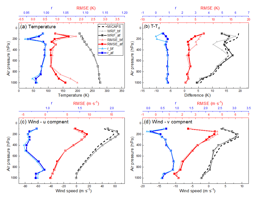
Figure 2MICAPS and simulated average temperature (a), dew point depression (b), and u (c) and v (d) components of wind during the simulation period (black lines), as well as RMSE (red lines) and spatial correlation coefficients (blue lines) between observations and simulations before and after assimilation for each vertical layer (subscripts “_bf” and “_af” represent simulation before and after assimilation).
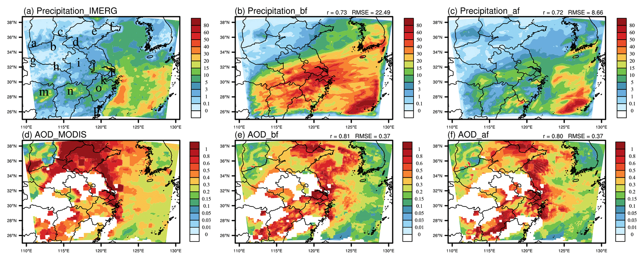
Figure 3Distributions of accumulated precipitation (unit: mm, a–c) and average AOD (dimensionless, d–f) during the simulation period from the observation and before and after assimilation of the meteorological fields. r and RMSE in the upper-right corner represent the spatial correlation coefficient and root-mean-square error of the observed and the simulated data, respectively, where RMSE is in the same unit as the variable in the figure. The subscripts “_bf” and “_af” in the subfigure captions have the same meaning as in Fig. 2. The markers a–p in Fig. 3a represent the locations of the stations in Fig. 4.
Spatial correlation analysis (Pearson product-moment coefficient), Pearson linear correlation analysis, and root-mean-square error (RMSE) are used to assess the spatial and temporal correlations of the simulated and observed values and to assess the error of the simulated values relative to the observations, respectively. To calculate these parameters, it is necessary to unify the spatiotemporal coordinates of the simulated and observed data. Specifically, MODIS (1–10 km resolution) and IMERG (0.1° resolution) data are interpolated to the WRF grid (12 km resolution) when comparing the model to satellite data, and WRF simulations are interpolated to the MICAPS grid (2.5° resolution) when comparing the model to MICAPS data.
Some screening criteria are applied to MODIS-retrieved cloud variables to make sure liquid clouds are selected (Saponaro et al., 2017), i.e., (1) selecting only liquid-phase cloud parameters and (2) filtering out transparent–cloudy pixels (COT < 5) to limit uncertainties (Zhang et al., 2012). The same filtering also applies to WRF-Chem model results when we evaluate the simulations against MODIS data. Cloud droplet number concentration (Nd) is calculated according to the approach of Brenguier et al. (2000) and Quaas et al. (2006):
where γ is an empirical constant with the value of m−5 and where COT and CER are obtained from MODIS. Moreover, due to the discontinuity of MODIS data, we matched the simulated data with MODIS data in spatiotemporal coordinates for evaluation (i.e., the simulated value is valid only when the MODIS data are valid in that spatiotemporal coordinate, otherwise the simulated value is set as missing and does not participate in the calculation). Due to the differences in satellite retrievals and model parameterization, the simulated liquid-phase clouds are often defined based on certain thresholds when being compared with satellite-retrieved data; e.g., Roh et al. (2020) classified the clouds with cloud liquid water content (CLWC) > 1 mg m−3 and cloud ice water content (CIWC) < 1 mg m−3 as liquid-phase clouds. In this study, based on the selection of column COT ≥ 5 that matched with MODIS filtering, the vertical layers (48 layers in total) with cloud optical thickness for water (COTW) > 0.1 and cloud optical thickness for ice (COTI) < 0.01 at each grid point and each time are selected as liquid-phase cloud layers, and the highest layer meeting this condition is defined as the simulated cloud top. This filtering is only used for comparison with MODIS data, and the analysis of aerosol–cloud interactions in liquid-phase clouds in this study is strictly limited to CLWC > 0 and CIWC = 0.
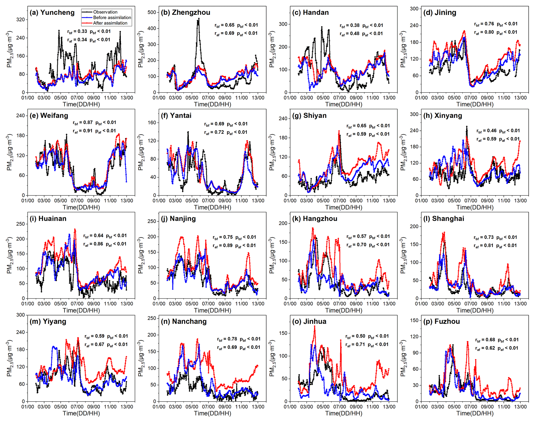
Figure 4Temporal variations in near-surface PM2.5 at each site, observed (black line) and simulated before (blue line) and after (red line) the assimilation of meteorological fields. The r and p values represent the correlation and significance of the observation and simulation, respectively, and subscripts “_bf” and “_af” have the same meaning as in the previous figures.
3.1 Evaluation of simulation result
Due to limitations in the resolution of observational data (e.g., MICAPS gridded upper-air meteorological field data with a resolution of 2.5°) and data availability (e.g., only terrestrial near-surface observations of PM2.5 are available), we utilized outer-domain simulations when evaluating the model results. For aerosol–cloud analysis in Sect. 3.3 and beyond, we employed finer inner-domain simulations.
Four-dimensional data assimilation directly impacts the simulations of meteorological fields (temperature, pressure, humidity, and wind) and thereby aerosols and clouds. Figure 2 presents the vertical distribution of meteorological variables from the simulations and observations along with the RMSE and spatial correlation coefficients of the simulations relative to observations at each layer. As the complexity of atmospheric physical and chemical processes and data errors resulted from processes such as observation and interpolation, the assimilation exerts some positive effects on the simulated meteorological field but also increases the difference between some of the simulated variables and the observations. Assimilation effectively improves the correlation between simulated and observed temperatures, dew point depression, middle-level zonal wind, and meridional wind, while it reduces the RMSE of simulated and observed temperatures, upper-level dew point depression, and lower- and upper-level meridional winds. At the same time, however, it also weakens the correlation between the simulated and observed low-level zonal winds and increases the RMSE of the simulated and observed mid-level dew point depression, upper-level zonal winds, and mid-level meridional winds. However, the assimilation is positive overall and provides effective help in exploring aerosol–cloud interactions.
Assimilation exerts indirect influences on precipitation, aerosol emission (mainly natural aerosols such as dust and sea salt), transport, and deposition. The RMSE of simulated and observed precipitation (Fig. 3a–c) is reduced by 61.5 % after assimilation. In terms of aerosol spatial distribution (Fig. 3d–f), the model reasonably reproduces the MODIS AOD distribution, and there is no significant difference in the simulated average AOD before and after assimilation. To further evaluate the effect of assimilation on the simulation of aerosol temporal variations, 16 stations with relatively continuous observation (Fig. 3a) are selected evenly from the model domain (Fig. 4). In general, the simulations before and after assimilation both reasonably reproduce the temporal variation in near-surface PM2.5, and the correlation between simulated and observed PM2.5 at all stations passes the test at 99 % significance. However, with assimilation, the simulated PM2.5 concentrations are generally closer to the observations, and the correlation coefficients between the simulated and the observed increase in 13 of the 16 stations, while the average correlation coefficient of the 16 stations increases from 0.63 to 0.69.
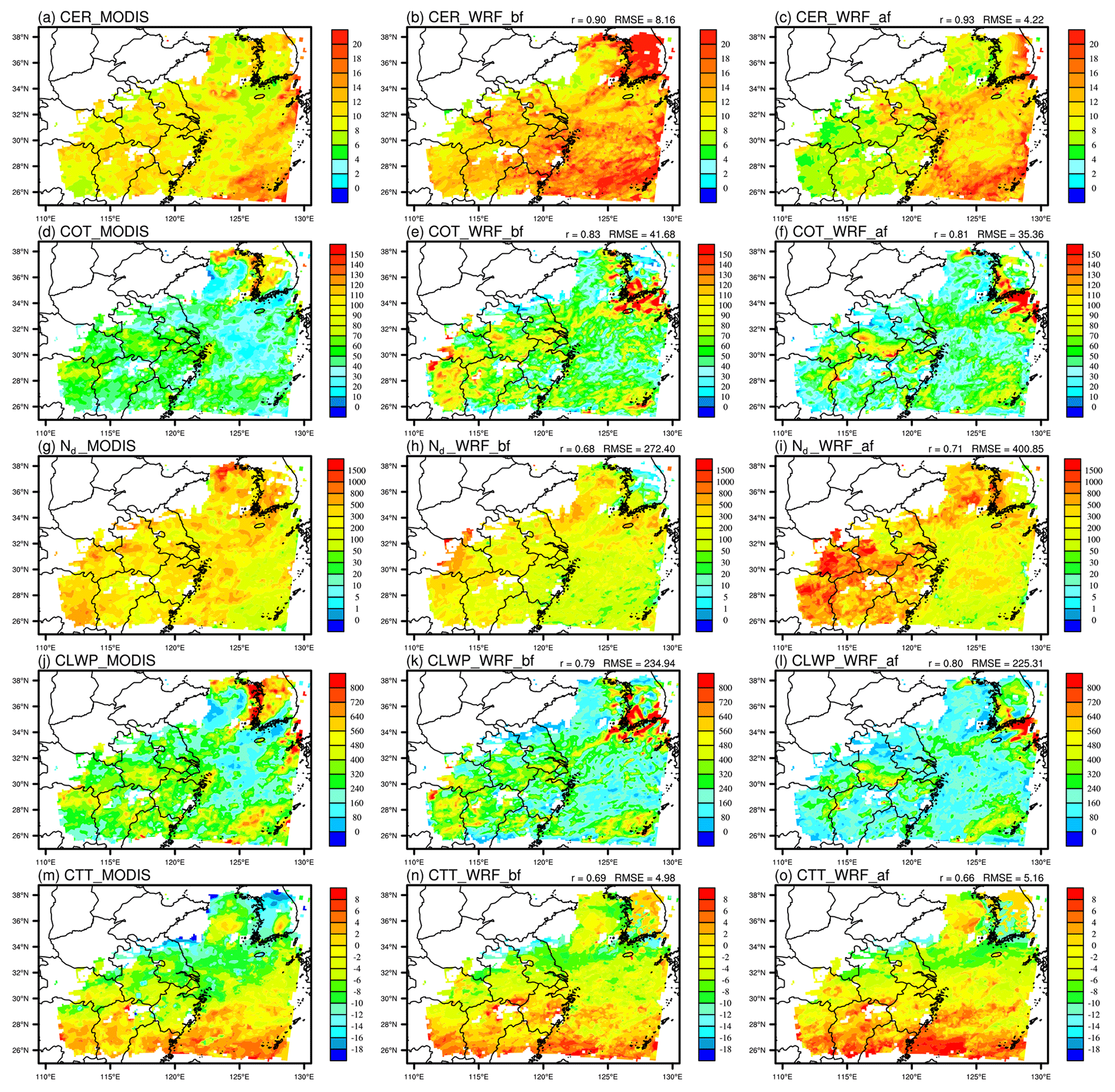
Figure 5Spatial distribution of average CER (a–c, in µm), COT (d–f, dimensionless), Nd (g–i, in cm−3), CLWP (j–l, in g m−2), and CTT (m–o, in °C) from MODIS and WRF simulation before and after assimilations. The r and RMSE in the upper-right corner and the subscripts “_bf” and “_af” in the subfigure captions have the same meaning as in the previous figures.
Figure 5 presents the simulated cloud parameters before and after assimilation and compared with MODIS. It is seen that the model without assimilation generally reproduces the spatial distribution of MODIS cloud parameters but with some overestimation for CER and COT and with some underestimation for Nd. Compared with MODIS, the simulation with assimilation produces overall higher Nd and lower CLWP over land but more reasonable CER and the distribution thereof. The model also reasonably reproduces the spatial distribution of MODIS-retrieved COT and CTT, which is important to our analysis presented below.
Based on the model samples matched with the spatiotemporal coordinates of MODIS valid values, we further evaluate the ability of the model to reproduce the satellite-retrieved CLWP–Nd relationship (Fig. 6). It is found that the simulation with assimilation generally reproduces the increase–decrease–increase variation in CLWP with Nd, although the model underestimates CLWP at low Nd, as shown by MODIS. The correlation between the simulation and the MODIS CLWP passes the test at the 99 % significance level (p<0.01). In contrast, the simulation before assimilation fails to reproduce the abovementioned CLWP-Nd relationship.
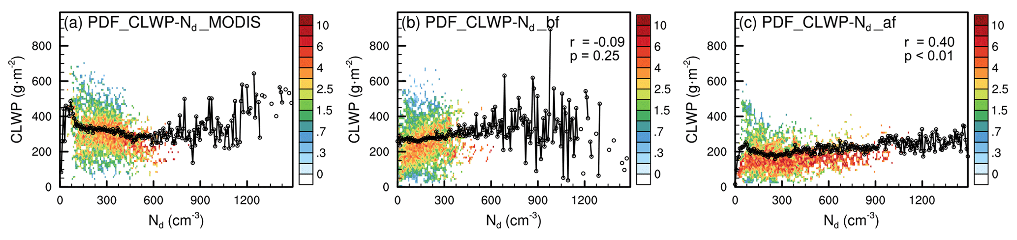
Figure 6CLWP–Nd relationship of MODIS (a) and simulated before (b) and after (c) assimilation. All samples are assigned into 200×100 bins, with each Nd value corresponding to 100 CLWP bins, and the colored dots in the figure represent the number of samples in that CLWP bin as a percentage of all the samples corresponding to that Nd value; i.e., each Nd value corresponds to a total of 100 % of the colored dot values. The black line in the figure represents the average of all samples corresponding to each Nd value.
3.2 Aerosol and cloud droplet distribution in EC and ECO
The aerosol physical and chemical processes, aerosol–cloud interactions, and consequent aerosol and cloud droplet distribution in EC and ECO (Fig. 7) exhibit distinct discrepancies due to the differences in aerosol properties, topography, and meteorological fields. EC aerosols are mainly primary and secondary aerosols produced by anthropogenic emissions (Fig. 8a), with small initial particle size. Under the influence of strong surface effects (surface longwave radiation cooling and terrain uplift) and intense updrafts, these small particles can be activated into cloud droplets, but the limited water vapor hinders further growth of cloud droplets. ECO aerosols are mainly transported from EC (as shown in Fig. 8b, ECO's locally emitted chloride and sodium aerosols contribute less than 20 % of the total aerosol mass) so that most aerosols in ECO are anthropogenic aerosols with mostly easily transportable small particles but with relatively more large particles compared to EC due to sea salt contribution. In addition, the abundant water vapor in ECO provides favorable conditions for aerosol activation and cloud droplet growth, with many more cloud droplets above 8 µm radius than in EC, though the total cloud droplet number is lower than in EC.
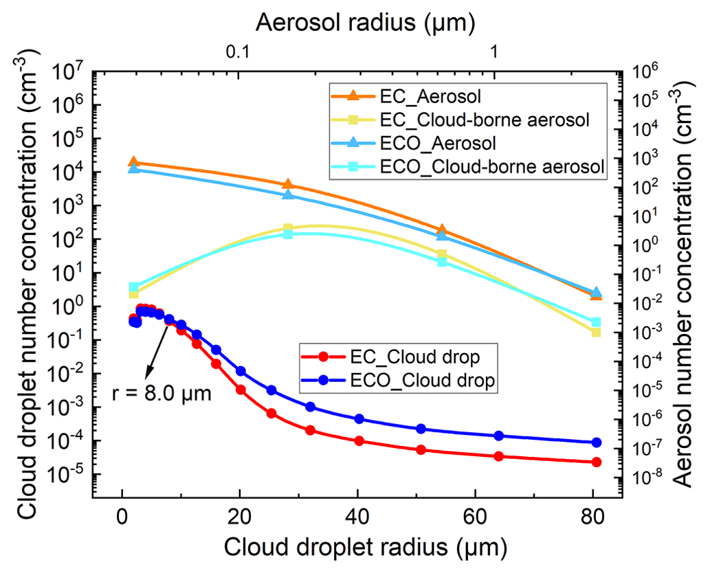
Figure 7Size distributions of cloud droplets, total aerosols, and activated (cloud-borne) aerosols in liquid-phase clouds of EC and ECO. In order to obtain the spectral distributions, the vertically weighted averages of the aerosol and cloud droplet number concentrations of each bin were first calculated as three-dimensional data containing only time, longitude, and latitude, and only the weighted averages of vertical layers of the liquid-phase cloud were calculated; i.e., the layers with CIWC > 0 were excluded from the calculations. Subsequent direct averaging of the three-dimensional number concentrations in each bin yielded the values in the figure.
EC aerosols mainly originate from surface emissions, so their number concentration (Naero) gradually decreases from the surface layer to the upper layer (Fig. 9a), while ECO aerosols are mainly transported from EC, so the Naero hotspot in ECO is located at the transport altitude near 1800 m above sea level (Fig. 9b). In addition to aerosol number and size, atmospheric supersaturation is a determinant of aerosol activation. In EC, the main contributing factors to supersaturation include (1) atmospheric convection, which acts mainly in the areas with relatively strong updrafts and high water vapor content below 4000 m altitude. Above 4000 m, the lack of water vapor makes it difficult to supersaturate even with strong updrafts (Fig. 9e, i, and k). (2) Water vapor and temperature changes caused by advection mainly work in the region of high water vapor content at tens of meters to 1000 m above the surface. (3) Long-wave radiative cooling at the surface, which acts mainly at night or in the early morning (Fig. S1 in the Supplement), leads to a high supersaturation of the atmosphere (the disappearance of this effect during the daytime makes the temporal average supersaturation near the surface relatively low). The high aerosol concentration and supersaturation makes the high Nd near the surface (Fig. 9c). (4) Topographic uplift, the forced uplift of topography, makes the atmosphere more susceptible to becoming supersaturated. In ECO, convection and advection are the main influencing factors for supersaturation. Due to the abundant water vapor content, even though vertical convection is weak, the relatively strong updraft area near 28° N at 2000–4000 m elevation generates much higher supersaturation than the EC does (Fig. 9e–f and i–l).
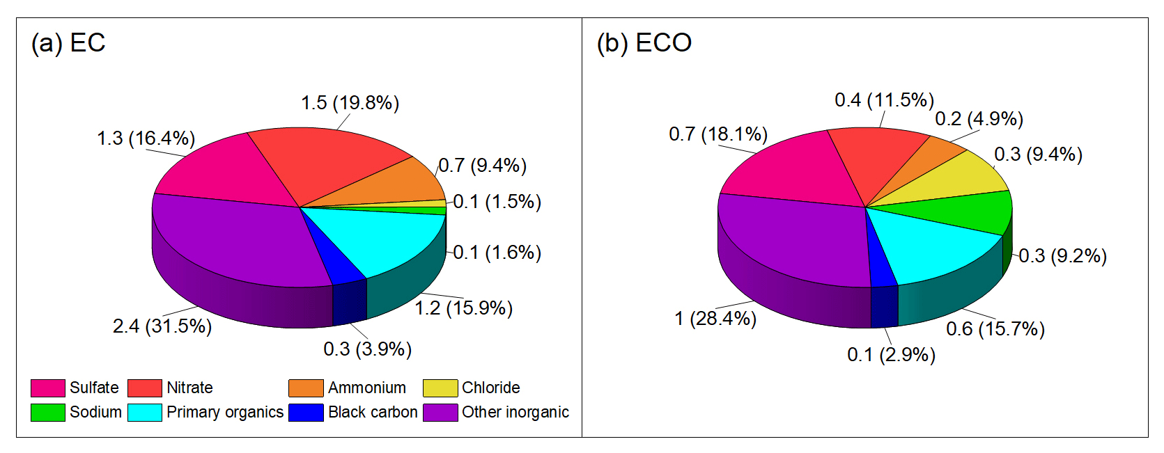
Figure 8Average concentration (in µg m−3) and percentage of each type of aerosol in EC and ECO during the simulation period (the concentration is a vertically weighted average of each type of aerosol).
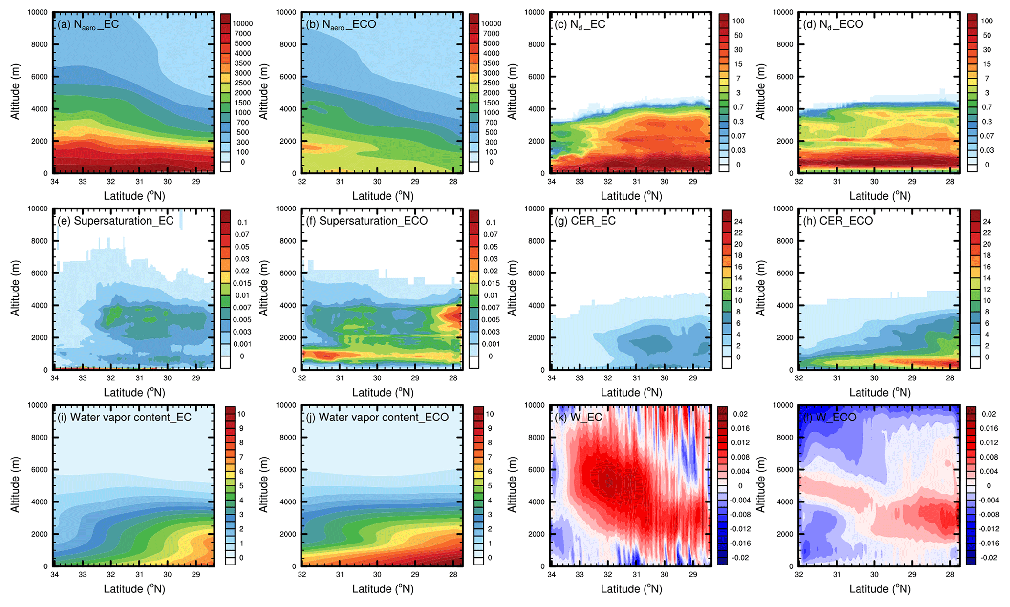
Figure 9EC and ECO aerosol number concentration (in cm−3, a–b), Nd in liquid-phase clouds (in cm−3, c–d), atmospheric supersaturation (in %, e–f), CER (in µm, g–h), water vapor content (in g m−3, i–j), and vertical wind speed (in m s−1, k–l) distributions. This figure presents how the latitude-averaged variables vary with the height. For Nd, supersaturation, and CER, we first filtered out the grid points with CIWC higher than 0. The lower limit of supersaturation value used in this study is 0. Even if the atmosphere is not saturated, the supersaturation value is 0 rather than a negative value. The average supersaturation characterizes the overall intensity of supersaturation in EC and ECO during the simulation period).
3.3 Aerosol activation of liquid-phase clouds in EC and ECO
To explore the responses of clouds to aerosols and their influencing factors, we perform a statistical analysis on aerosols, clouds, and meteorological elements for the grid points with liquid-phase clouds (i.e., Nd>1 cm−3, CIWC = 0, and supersaturation > 0) at each time. The statistics are based on each vertical layer and on the column (vertical integration of layers with liquid-phase clouds), respectively, with the former providing abundant samples and more immediate and detailed aerosol–cloud relationships and the latter facilitating relevant studies to compare it directly with information such as satellite retrievals.
Aerosol activation is the first step of aerosol–cloud interaction, and we analyze the variation in Nd with aerosol (Fig. 10) based on the statistics for each vertical layer and for the column, respectively. At low Naero, aerosols promote cloud droplet increase by acting as CCN (Fig. 10a–b). As aerosols and cloud droplets increase, more small aerosols (Fig. 10e–f) heighten the requirement of atmospheric supersaturation for aerosol activation, and the consumption of water vapor from cloud droplet growth makes it more difficult for the atmosphere to reach supersaturation, thus suppressing aerosol activation. As shown in Fig. 10a–b, Nd in both EC and ECO exhibit the general trend of increasing first and then decreasing with increasing Naero, but there are some differences between EC and ECO. In EC (Fig. 10a), strong surface effects and updrafts, as well as abundant aerosols, allow Nd to maintain a more persistent trend. In addition, aerosol activation is not suppressed in the near-surface areas with high aerosol concentration, and aerosols can still be activated at high supersaturation (Fig. 10i) caused by the effects of longwave radiative cooling (the diurnal variation in this effect is also one of the main reasons for the fluctuation of Nd with Naero), terrain uplift (the high-topographic-gradient areas where this action takes effect are usually also characterized by aerosol accumulation), and relatively high water vapor content (Fig. 10m) near the surface. In ECO, weaker updrafts and the absence of surface effects (as in EC) limit its supersaturated water supply, and the supersaturation (Fig. 10f) shows a more pronounced and synchronized variation with variation in ambient water vapor content (Fig. 10n) and decreases rapidly with increasing Naero after the Nd peak. After Nd reaches its peak, the increase in small aerosols and the decrease in supersaturation prevent Nd from continuing to increase and Nd starts to show a decreasing trend, without fluctuations like in EC. Unlike the statistics for each vertical layer, the statistics for the column show that Nd exhibits an increase with AOD followed by a general maintenance (Fig. 10c–d). In EC, the maintenance is mainly due to a higher percentage of easily activated large particles at high AOD (Fig. 10g), while in ECO it is mainly due to an overall higher supersaturation (Fig. 10l) associated with the abundant water vapor. Because column sampling cannot accurately match aerosol–cloud-related variables in vertical coordinates based on the intensity of cloud processes, column sampling exhibits a less immediate and precise relationship between supersaturation and water vapor content than the sampling of each vertical layer does. So, in terms of column statistics, although ECO water content is close to EC, its average supersaturation is much higher than that of EC.
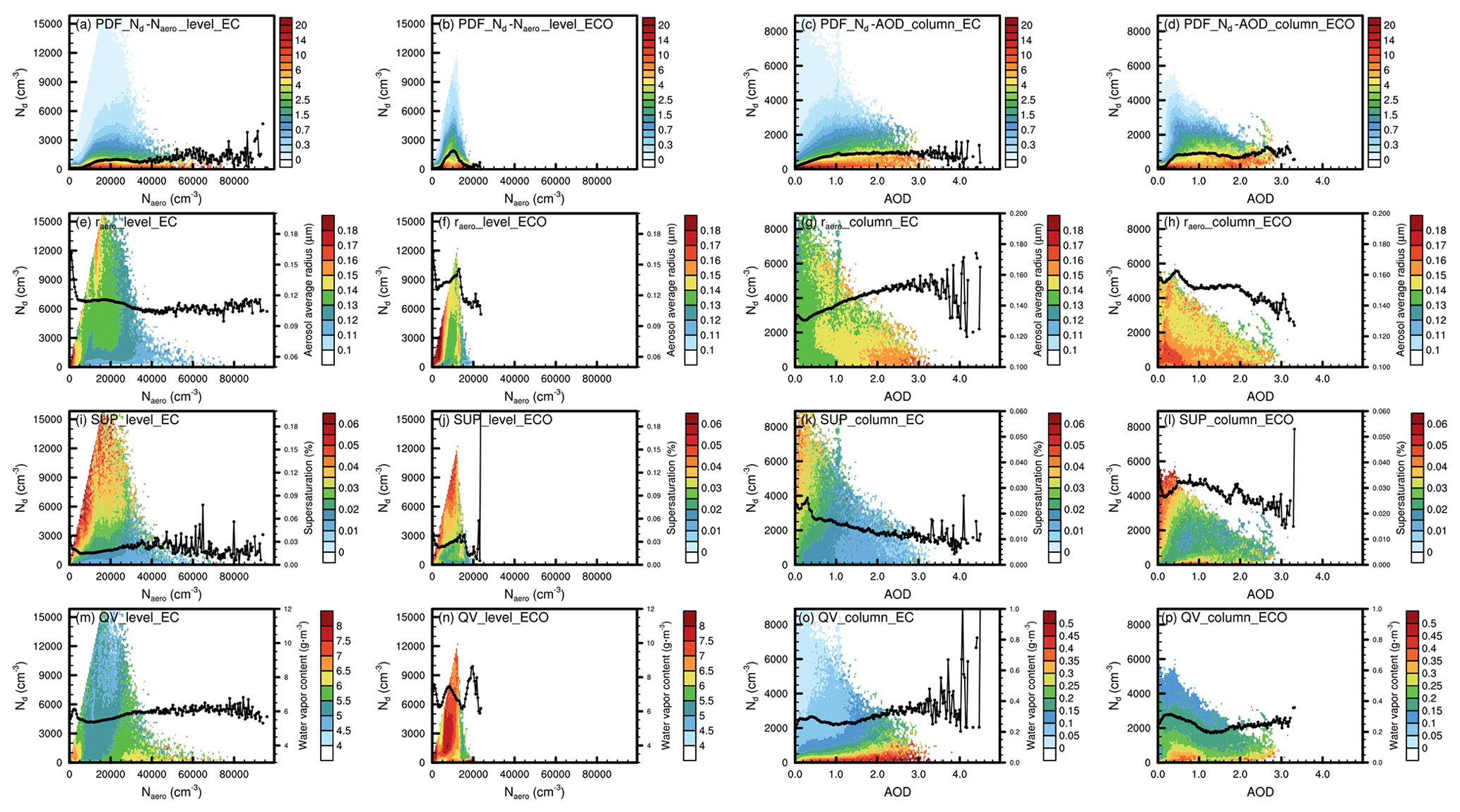
Figure 10Nd varies with aerosols (a–d; the unit for colored dots is %, while the unit for the black lines is the unit on the left vertical axis) and with the aerosol volume average radius (e–h; the colored dots and black lines of these figures and all subsequent figures correspond to the units on the right vertical axis). Supersaturation (i–l) and water vapor content (m–p) vary with Nd and aerosols in EC and ECO based on statistics at each vertical layer (two columns on the left) and column (two columns on the right), respectively. Samples were taken from each time and each grid point, and each sample contained Naero or AOD, Nd, aerosol volume mean radius, supersaturation, and water vapor content values. These samples were placed into 200 aerosol ×100 Nd bins according to the interval in which their Naero or AOD values and Nd values were located. The colored dots in panels (a)–(d) represent the proportion of that bin's sample number to the total number of samples of the 100 bins corresponding to the Naero or AOD interval; i.e., the total value of all colored dots corresponding to each Naero or AOD interval is 100 %. The black lines in panels (a)–(d) represent the average Nd of all samples at the corresponding Naero or AOD intervals. The colored dots in panels (e)–(p) represent the average values of the variable for all samples in the bin corresponding to the aerosol and Nd intervals. The black lines in panels (e)–(p) represent the average value of this variable in all samples corresponding to this aerosol interval.
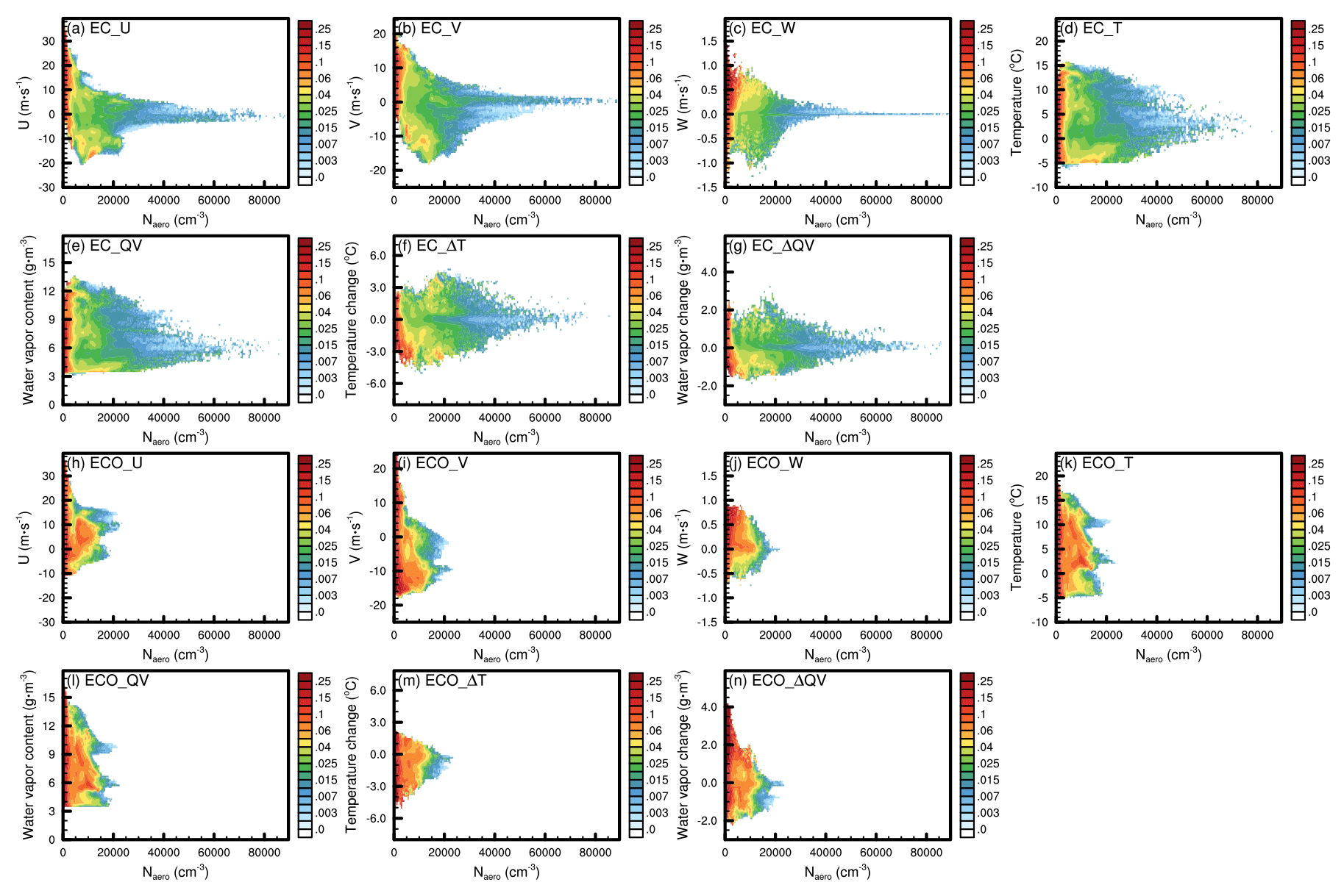
To investigate the influence of meteorological conditions on aerosol activation, a statistical analysis is presented in Fig. 11 on the variation in the Nd-to-Naero ratio (characterizing the intensity of aerosol activation) with Naero for different zonal wind speed (U), meridional wind speed (V), vertical wind speed (W), temperature, and water vapor content, as well as changes in temperature and water vapor per hour. In EC, a high Nd-to-Naero ratio occurs when the zonal wind speed is < −6 m s−1 or the meridional wind speed is < −7 m s−1, with the former due to large amounts of water vapor from the ocean brought by easterly winds (Fig. S2b) and the latter due to cold air brought by northerly winds (Fig. S2a) and uplift caused by the south high and north low topography in EC (Fig. 1). The overall high ratio is exhibited at relatively high vertical wind speeds, but aerosol activation is also found when the vertical airflow is weak or dominated by downdraft due to the influence of advection at tens of meters to 1000 m above the surface, topographic uplift, and long-wave radiative cooling at the surface. A high Nd-to-Naero ratio in EC mainly occurs at low temperatures and in low-humidity conditions, which is due to the fact that the temperature and humidity horizontal gradients are essentially the same (Fig. S2), and EC with low overall water vapor content is more likely to reach supersaturation at both low temperatures and low water vapor content, and it becomes increasingly difficult to reach supersaturation when the temperature and humidity are simultaneously increased. The increase in water vapor and decrease in temperature contribute to EC aerosol activation, but the strong surface effects and updrafts enable aerosol activation to occur even at significant warming or humidity reduction.
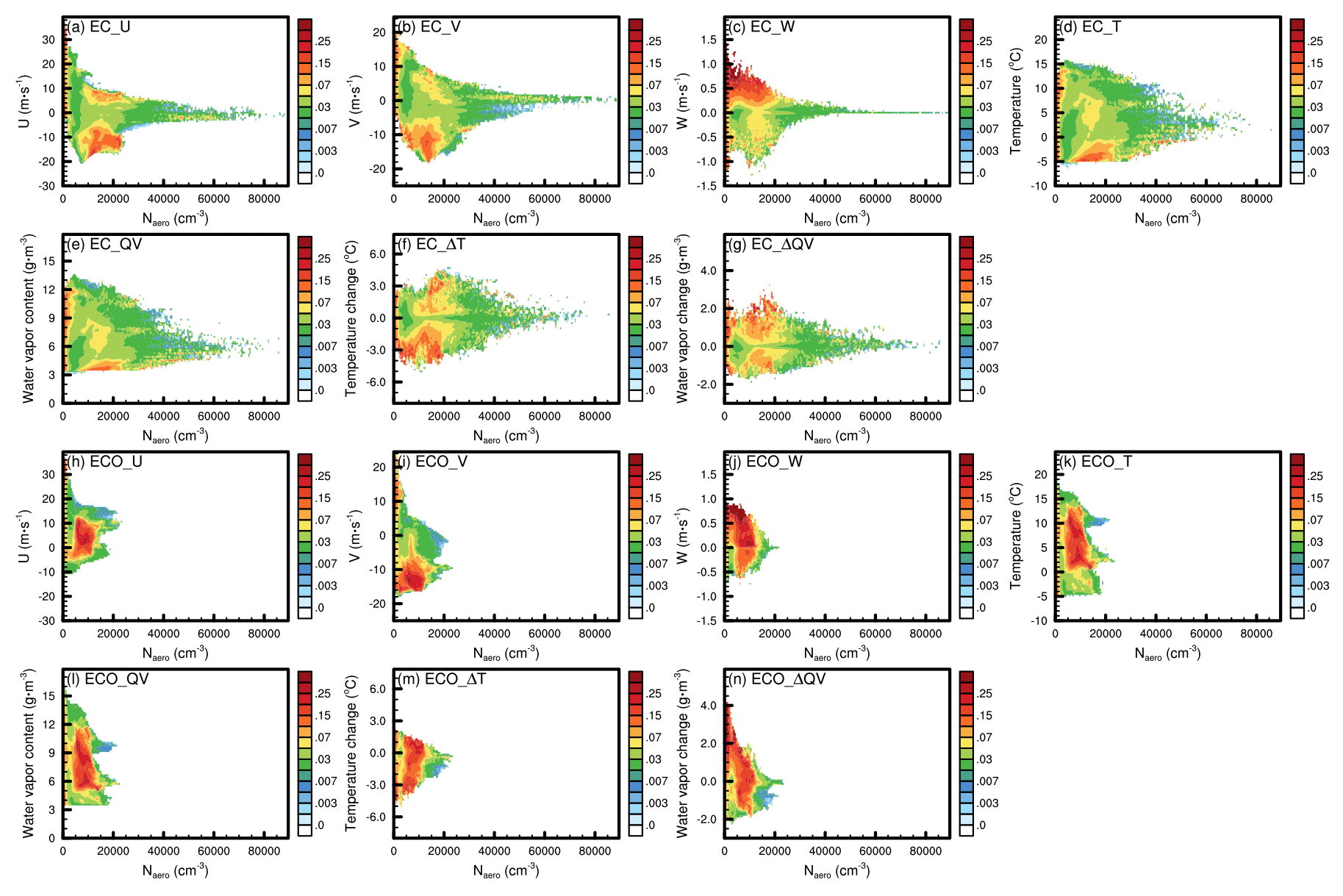
Figure 11Variation in EC (a–g) and ECO (h–n) Nd-to-Naero ratio (unit: cm−3 cm3) with Naero at different U (a and h), V (b and i), W (c and j), temperature (d and k), water vapor content (e and l), temperature change (f and m), and water vapor change (g and n). This figure is sampled at each vertical layer and is calculated in the same way as in Fig. 10 except that the bin of Nd is replaced by the bin of each meteorological element.
In ECO, the zonal wind speed favorable to aerosol activation is below 0 or 0–13 m s−1, with the former ensuring the supply of water vapor and the latter providing more abundant aerosols, while, at zonal wind speed above 13 m s−1, the excessively dry air from land makes the atmosphere difficult to reach supersaturation, despite the large aerosol amounts brought by the westerly wind. The meridional wind speed suitable for ECO activation is mainly below −8 m s−1, with the cold air brought by strong northerly winds making it easier for the atmosphere to reach supersaturation. The abundance of water vapor makes ECO more susceptible to reaching supersaturation by updrafts, making its activation exhibit a high sensitivity to vertical wind speeds. Compared to EC, ECO's more abundant water vapor content generates a higher Nd-to-Naero ratio at higher temperatures and in high-humidity conditions. In addition, ECO aerosol activation is more limited by cooling and humidification due to atmospheric motion (no strong surface effects like in EC), and its high Nd-to-Naero ratio is clearly skewed toward high-humidification and high-cooling conditions compared to EC.
3.4 Impact of aerosols on development of liquid-phase clouds
Aerosol activation alters cloud droplet size distribution and consequent changes in cloud microphysical and dynamical processes, which is also known as rapid adjustment (Heyn et al., 2017; Mulmenstadt and Feingold, 2018). We discuss the variations in CLWC and CER with increasing Nd (Fig. 12) for precipitation clouds (rainwater content above 1 mg m−3 for each vertical layer and above 1 g m−2 for the column) and non-precipitating clouds (rainwater content below 0.001 mg m−3 for each vertical layer and below 0.001 g m−2 for the column). For precipitation clouds, CLWC in both EC and ECO shows a trend of rapid increase followed by a gradual slowdown (the net influence of water content limitation, evaporation, and precipitation effects, accompanied by the decrease in CER) in Nd. The difference lies in the fact that the abundant water vapor in ECO makes its CLWC increase much faster than in EC when Nd is very low, whereas the higher aerosol concentration, strong surface effects, and strong updrafts in EC enable it to have a wider Nd range and produce higher CLWC. For non-precipitating clouds, the consumption of limited supersaturated water by aerosol activation and cloud droplet growth causes clear decreasing trends in CLWC with Nd after CLWC increasing to a certain level. The difference between the two regions is that more limited supersaturated water supply in ECO causes its CER to decrease faster and CLWC to start decreasing earlier.
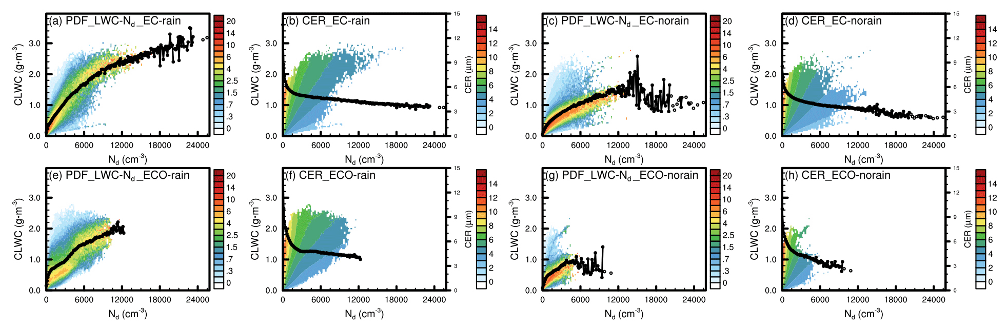
Figure 12CLWC varies with Nd (a, c, e, g), and CER varies with CLWC and Nd (b, d, f, h) for precipitating (two columns on the left) and non-precipitating (two columns on the right) clouds in EC (a–d) and ECO (e–h), based on statistics at each vertical layer. The interpretation of this figure is the same as for Fig. 10.
We further examine the variations in CLWP and its related elements with AOD based on the statistics of the column (Fig. 13). For the precipitation clouds, with the increase in AOD, CLWP remains generally stable (the combined effects of cloud droplets and precipitation changes), while Nd increases initially and then decreases (the decrease in Nd of ECO at AOD 1.5–2.0 is due to a decrease in water vapor content caused by individual processes as shown in Fig. 10p, and simulations and statistical analyses for longer time periods can attenuate the effect of such individual processes), and both CER and rainwater path (RWP; i.e., rainwater column content) decrease. There is a bi-directional interaction between RWP and aerosols (i.e., low AOD is largely resulted from the washout of aerosols by precipitation), whereas increasing Nd and decreasing CER due to increasing aerosols also decrease the RWP. For non-precipitation clouds, CLWP increases with AOD, while Nd firstly increases and then shows a weak decreasing trend.
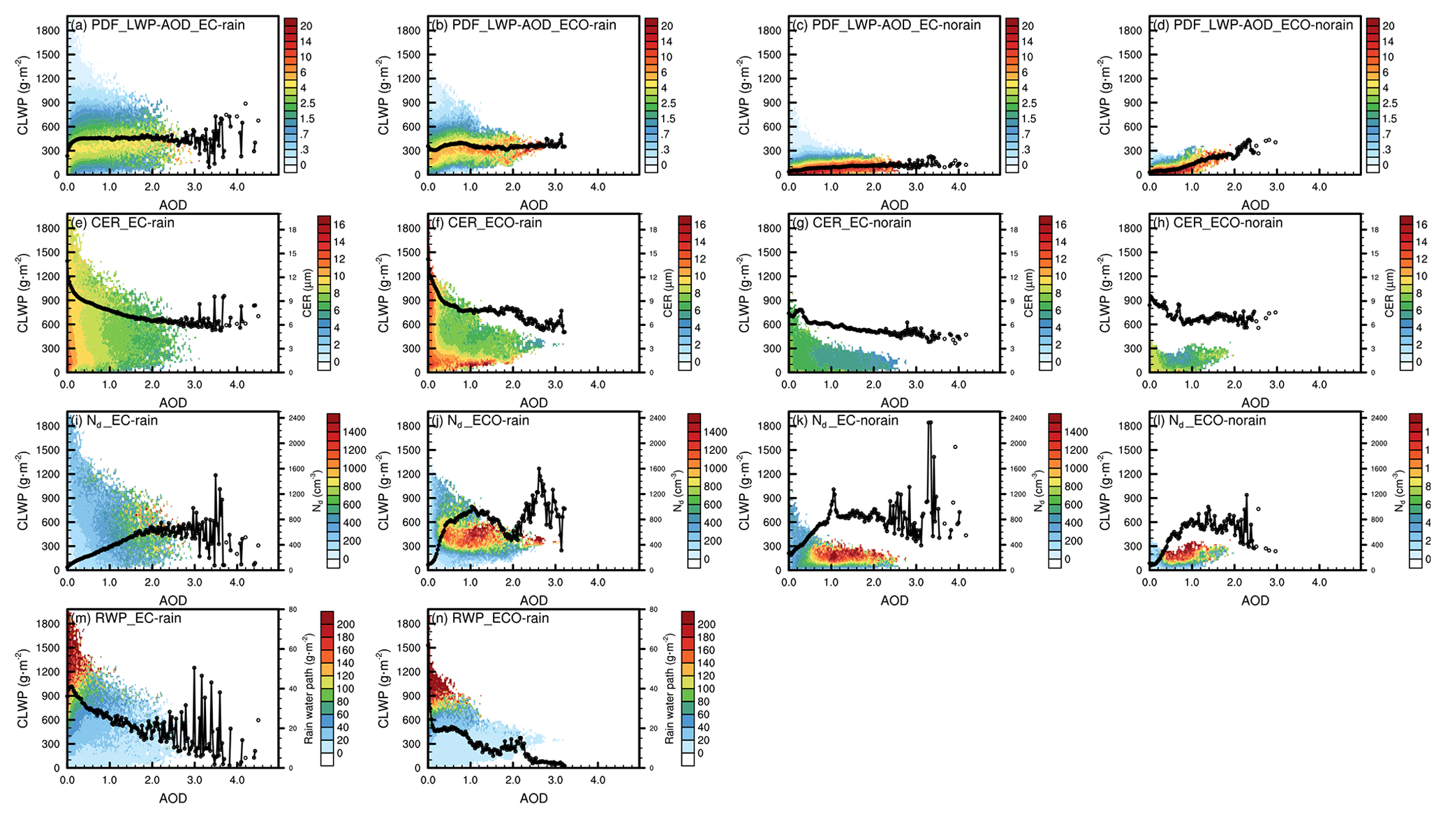
Figure 13CLWP varies with AOD (a–d) and CER (e–h). Nd (i–l) and RWP (m–n) vary with CLWP and AOD for precipitation clouds (two columns on the left) and non-precipitating clouds (two columns on the right) in EC and ECO. The interpretation of this figure is the same as for Fig. 10).
Figure 14 exhibits the effects of different meteorological and aerosol conditions on CLWC. The CLWC and Naero ratio (characterizing the speed of cloud development) under different meteorological and Naero conditions shows generally similar variation to the Nd and Naero ratio in Fig. 11, with only some minor differences. Compared to the high Nd and Naero ratios exhibited in Fig. 10, which tend to occur at medium Naero, the high CLWC and Naero ratios at low Naero are more heavily weighted due to the more abundant water vapor supply and weaker evaporation when there are fewer but larger cloud droplets.
In this study, aerosol–cloud interactions in liquid-phase clouds over eastern China (EC) and its adjacent ocean region (ECO) in winter are explored based on the WRF-Chem–SBM model in which a spectral-bin microphysics (SBM) scheme and an online aerosol module (MOSAIC) are coupled.
The impact of four-dimensional data assimilation on the simulation and performance of the coupling system is firstly evaluated using multiple observations. With assimilation, the simulated meteorological field is generally closer to the observations both in values and in spatial distribution. The simulations of precipitation and aerosols are effectively improved by optimizing the meteorological field, the RMSE of simulated precipitation versus observation is reduced by 61.5 %, and the temporal correlation of simulated PM2.5 with observations at each site is improved by 9.5 % on average.
We explore the responses of clouds to aerosols and their influencing factors through the statistics of liquid-phase cloud samples. Statistics on each vertical layer show that, in both EC and ECO, Nd exhibits an overall increasing and then decreasing trend with Naero. The difference is that the strong surface effects (surface longwave radiation cooling and terrain uplift) in EC induce high Nd near the surface with high Naero, whereas, in ECO, Nd increases faster at low Naero due to abundant water vapor and decreases rapidly after the peak of Nd. However, the statistics on the entire column show that Nd increases with AOD and then generally remains unchanged (there is no clear decrease as in the statistics on each vertical layer), partly because high AOD does not correspond to high Naero and also because the statistics on column are not as detailed and immediate as those on each vertical layer.
Statistics on each vertical layer show that, in precipitation clouds, CLWC increases with Nd and its increase rate gradually slows down, whereas, in non-precipitation clouds with lower water content, CLWC decreases with Nd after its increase to the peak. The difference between EC and ECO precipitation clouds lies in the fact that the abundant aerosols, strong surface effects, and strong updrafts allow EC to produce higher Nd and CLWC, and the more abundant water vapor in ECO enables its CLWC to increase faster at low Nd. The difference between the non-precipitating clouds in the two regions is that the insufficient supply of supersaturated water due to fewer and less intense processes affecting supersaturation in ECO leads to its CER decreasing rapidly, and the CLWC begins to decrease at lower Nd than in EC. We further analyze the variation in CLWP with AOD based on the statistics of the column. For precipitation clouds, CLWP remains generally stable with AOD without significant variation due to the combined effect of precipitation and aerosols, while in non-precipitating clouds, which are almost unaffected by precipitation, CLWP increases gradually with AOD.
We explore the effects of different meteorological and aerosol conditions on the Nd-to-Naero ratio (characterizing the intensity of aerosol activation) and on the CLWC-to-Naero ratio (characterizing the speed of cloud development). In EC, favorable meteorological conditions for aerosol activation include (1) moist air brought by strong easterly winds, (2) cooling and topographic uplift due to strong northerly winds, and (3) strong updraft. In ECO, the meteorological conditions suitable for aerosol activation include (1) aerosol-rich and not excessive dry airflow from moderate westerly winds, (2) cooling due to strong northerly winds, and (3) strong updraft. ECO's abundant water vapor allows it to produce a high Nd-to-Naero ratio in higher-temperature environments than EC, but fewer and less intense processes affecting supersaturation make its activation more dependent on strong humidification and cooling (whereas EC's strong surface effects can enable a high Nd-to-Naero ratio to occur even under significant warming or humidity reduction). Meteorological conditions suitable for CLWC increase are close to aerosol activation, while high CLWC-to-Naero ratios occur more often in low-Naero conditions compared to moderate-Naero conditions where a high Nd-to-Naero ratio appears.
The WRF-Chem model code can be downloaded from https://www2.mmm.ucar.edu/wrf/users/download/get_sources.html (University Corporation for Atmospheric Research, 2024). The WRF-Chem–SBM model code can be obtained by contacting Jiwen Fan of Argonne National Laboratory. The model outputs are available upon request (the namelist file of the model simulation is attached as Supplement A). NCEP data sets (https://doi.org/10.5065/39C5-Z211, Satellite Services Division et al., 2004; https://doi.org/10.5065/4F4P-E398, NCEP et al., 2004; https://doi.org/10.5065/D65Q4T4Z, NCEP et al., 2015), CAM-chem model output (https://doi.org/10.5065/NMP7-EP60, Buchholz et al., 2019; https://doi.org/10.1029/2019MS001882, Emmons et al., 2020), MICAPS meteorological fields (http://www.nmc.cn, National Meteorological Centre of China, 2009), near-surface PM2.5 observations (https://air.cnemc.cn:18007, China National Environmental Monitoring Center, 2023), IMERG precipitation (https://doi.org/10.5067/GPM/IMERGDF/DAY/06, Huffman et al., 2019), and MODIS aerosol (https://doi.org/10.5067/MODIS/MOD04_L2.061, Levy et al., 2017) and cloud (https://doi.org/10.5067/MODIS/MOD06_L2.061, Platnick et al., 2017) data can be accessed from the corresponding websites or references.
The supplement related to this article is available online at: https://doi.org/10.5194/acp-24-9101-2024-supplement.
JZ and XM designed and conducted the model experiments, analyzed the results, and wrote the paper. XM developed the project idea and supervised the project. XM, JQ, and HJ proposed scientific suggestions and revised the paper.
At least one of the (co-)authors is a member of the editorial board of Atmospheric Chemistry and Physics. The peer-review process was guided by an independent editor, and the authors also have no other competing interests to declare.
Publisher's note: Copernicus Publications remains neutral with regard to jurisdictional claims made in the text, published maps, institutional affiliations, or any other geographical representation in this paper. While Copernicus Publications makes every effort to include appropriate place names, the final responsibility lies with the authors.
This study is supported by the Second Tibetan Plateau Scientific Expedition and Research (STEP) program (grant no. 2019QZKK0103), the National Natural Science Foundation of China (grant nos. 42061134009 and 41975002), and the Postgraduate Research and Practice Innovation Program of Jiangsu Province (grant no. KYCX22_1151). The numerical calculations in this paper were conducted in the High-Performance Computing Center of Nanjing University of Information Science & Technology. We express our gratitude to Dr. Jiwen Fan of Argonne National Laboratory for providing the code for the WRF-Chem–SBM model and Prof. Qian Chen of Nanjing University of Information Science & Technology for providing advice on this study. We are grateful to the National Aeronautics and Space Administration, the National Centers for Environmental Prediction, the MEIC support team, the Chinese National Meteorological Center, and the China National Environmental Monitoring Center for providing the MODIS and GPM data, FNL and observation subsets, MEIC emission inventory, MICAPS data, and PM2.5 data, respectively.
This research has been supported by the Second Tibetan Plateau Scientific Expedition and Research (STEP) program (grant no. 2019QZKK0103), the National Natural Science Foundation of China (grant nos. 42061134009 and 41975002), and the Postgraduate Research and Practice Innovation Program of Jiangsu Province (grant no. KYCX22_1151).
This paper was edited by Xiaohong Liu and reviewed by two anonymous referees.
Albrecht, B. A.: Aerosols, cloud microphysics, and fractional cloudiness, Science 245, 1227–1230, https://doi.org/10.1126/science.245.4923.1227, 1989.
Arias, P., Bellouin, N., Coppola, E., Jones, R., Krinner, G., Marotzke, J., Naik, V., Palmer, M., Plattner, G.-K., Rogelj, J., Rojas, M., Sillmann, J., Storelvmo, T., Thorne, P., Trewin, B., Achutarao, K., Adhikary, B., Allan, R., Armour, K., Bala, G., Barimalala, R., Berger, S., Canadell, J. G., Cassou, C., Cherchi, A., Collins, W. D., Collins, W. J., Connors, S., Corti, S., Cruz, F., Dentener, F. J., Dereczynski, C., Di Luca, A., Diongue Niang, A., Doblas-Reyes, P., Dosio, A., Douville, H., Engelbrecht, F., Eyring, V., Fischer, E. M., Forster, P., Fox-Kemper, B., Fuglestvedt, J., Fyfe, J., Gillett, N., Goldfarb, L., Gorodetskaya, I., Gutierrez, J. M., Hamdi, R., Hawkins, E., Hewitt, H., Hope, P., Islam, A. S., Jones, C., Kaufmann, D., Kopp, R., Kosaka, Y., Kossin, J., Krakovska, S., Li, J., Lee, J.-Y., Masson-Delmotte, V., Mauritsen, T., Maycock, T., Meinshausen, M., Min, S.-K., Ngo Duc, T., Otto, F., Pinto, I., Pirani, A., Raghavan, K., Ranasighe, R., Ruane, A., Ruiz, L., Sallée, J.-B., Samset, B. H., Sathyendranath, S., Monteiro, P. S., Seneviratne, S. I., Sörensson, A. A., Szopa, S., Takayabu, I., Treguier, A.-M., van den Hurk, B., Vautard, R., Von Schuckmann, K., Zaehle, S., Zhang, X., and Zickfeld, K.: Climate Change 2021: The Physical Science Basis. Contribution of Working Group I to the Sixth Assessment Report of the Intergovernmental Panel on Climate Change; Technical Summary, The Intergovernmental Panel on Climate Change AR6, Remote, 33–144, https://doi.org/10.1017/9781009157896.002, 2021.
Arola, A., Lipponen, A., Kolmonen, P., Virtanen, T. H., Bellouin, N., Grosvenor, D. P., Gryspeerdt, E., Quaas, J., and Kokkola, H.: Aerosol effects on clouds are concealed by natural cloud heterogeneity and satellite retrieval errors, Nat. Commun., 13, 1–8, https://doi.org/10.1038/s41467-022-34948-5, 2022.
Bangert, M., Kottmeier, C., Vogel, B., and Vogel, H.: Regional scale effects of the aerosol cloud interaction simulated with an online coupled comprehensive chemistry model, Atmos. Chem. Phys., 11, 4411–4423, https://doi.org/10.5194/acp-11-4411-2011, 2011.
Bao, J. W., Feng, J. M., and Wang, Y. L.: Dynamical downscaling simulation and future projection of precipitation over China, J. Geophys. Res.-Atmos., 120, 8227–8243, https://doi.org/10.1002/2015jd023275, 2015.
Brenguier, J. L., Pawlowska, H., Schüller, L., Preusker, R., Fischer, J., and Fouquart, Y.: Radiative properties of boundary layer clouds: Droplet effective radius versus number concentration, J. Atmos. Sci., 57, 803–821, https://doi.org/10.1175/1520-0469(2000)057<0803:RPOBLC>2.0.CO;2, 2000.
Bretherton, C. S., Blossey, P. N., and Uchida, J.: Cloud droplet sedimentation, entrainment efficiency, and subtropical stratocumulus albedo, Geophys. Res. Lett., 34, L03813, https://doi.org/10.1029/2006gl027648, 2007.
Buchholz, R. R., Emmons, L. K., Tilmes, S., and The CESM2 Development Team: CESM2.1/CAM-chem Instantaneous Output for Boundary Conditions, UCAR/NCAR – Atmospheric Chemistry Observations and Modeling Laboratory [data set], https://doi.org/10.5065/NMP7-EP60, 2019.
Carslaw, K. S., Boucher, O., Spracklen, D. V., Mann, G. W., Rae, J. G. L., Woodward, S., and Kulmala, M.: A review of natural aerosol interactions and feedbacks within the Earth system, Atmos. Chem. Phys., 10, 1701–1737, https://doi.org/10.5194/acp-10-1701-2010, 2010.
Chen, Y. C., Christensen, M. W., Stephens, G. L., and Seinfeld, J. H.: Satellite-based estimate of global aerosol-cloud radiative forcing by marine warm clouds, Nat. Geosci., 7, 643–646, https://doi.org/10.1038/ngeo2214, 2014.
Chen, Y. Y., Yang, K., Zhou, D. G., Qin, J., and Guo, X. F.: Improving the Noah Land Surface Model in Arid Regions with an Appropriate Parameterization of the Thermal Roughness Length, J. Hydrometeorol., 11, 995–1006, https://doi.org/10.1175/2010jhm1185.1, 2010.
China National Environmental Monitoring Center: National Urban Air Quality Real-time Publishing Platform, https://air.cnemc.cn:18007 (last access: 19 March 2023), 2023.
Christensen, M. W. and Stephens, G. L.: Microphysical and macrophysical responses of marine stratocumulus polluted by underlying ships: 2. Impacts of haze on precipitating clouds, J. Geophys. Res.-Atmos., 117, D11203, https://doi.org/10.1029/2011jd017125, 2012.
Christensen, M. W., Chen, Y. C., and Stephens, G. L.: Aerosol indirect effect dictated by liquid clouds, J. Geophys. Res.-Atmos., 121, 14636–614650, https://doi.org/10.1002/2016JD025245, 2016.
Christensen, M. W., Gettelman, A., Cermak, J., Dagan, G., Diamond, M., Douglas, A., Feingold, G., Glassmeier, F., Goren, T., Grosvenor, D. P., Gryspeerdt, E., Kahn, R., Li, Z., Ma, P.-L., Malavelle, F., McCoy, I. L., McCoy, D. T., McFarquhar, G., Mülmenstädt, J., Pal, S., Possner, A., Povey, A., Quaas, J., Rosenfeld, D., Schmidt, A., Schrödner, R., Sorooshian, A., Stier, P., Toll, V., Watson-Parris, D., Wood, R., Yang, M., and Yuan, T.: Opportunistic experiments to constrain aerosol effective radiative forcing, Atmos. Chem. Phys., 22, 641–674, https://doi.org/10.5194/acp-22-641-2022, 2022.
Church, J., Clark, P., Cazenave, A., Gregory, J., and Unnikrishnan, A.: Climate Change 2013: The Physical Science Basis, Contribution of Working Group I to the Fifth Assessment Report of the Intergovernmental Panel on Climate Change, Computational Geometry, https://doi.org/10.1016/S0925-7721(01)00003-7, 2013.
Emmons, L. K., Schwantes, R. H., Orlando, J. J., Tyndall, G., Kinnison, D., Lamarque, J., Marsh, D., Mills, M. J., Tilmes, S., and Bardeen, C.: The chemistry mechanism in the community earth system model version 2 (CESM2), J. Adv. Model. Earth Syst., 12, e2019MS001882, https://doi.org/10.1029/2019MS001882, 2020.
Fan, J. W., Leung, L. R., Li, Z. Q., Morrison, H., Chen, H. B., Zhou, Y. Q., Qian, Y., and Wang, Y.: Aerosol impacts on clouds and precipitation in eastern China: Results from bin and bulk microphysics, J. Geophys. Res.-Atmos., 117, D00K36, https://doi.org/10.1029/2011jd016537, 2012.
Fan, J. W., Liu, Y. C., Xu, K. M., North, K., Collis, S., Dong, X. Q., Zhang, G. J., Chen, Q., Kollias, P., and Ghan, S. J.: Improving representation of convective transport for scale-aware parameterization: 1. Convection and cloud properties simulated with spectral bin and bulk microphysics, J. Geophys. Res.-Atmos., 120, 3485–3509, https://doi.org/10.1002/2014jd022142, 2015.
Fast, J. D., Gustafson, W. I., Easter, R. C., Zaveri, R. A., Barnard, J. C., Chapman, E. G., Grell, G. A., and Peckham, S. E.: Evolution of ozone, particulates, and aerosol direct radiative forcing in the vicinity of Houston using a fully coupled meteorology-chemistry-aerosol model, J. Geophys. Res.-Atmos., 111, D21305, https://doi.org/10.1029/2005jd006721, 2006.
Fuentes, E., Coe, H., Green, D., and McFiggans, G.: On the impacts of phytoplankton-derived organic matter on the properties of the primary marine aerosol – Part 2: Composition, hygroscopicity and cloud condensation activity, Atmos. Chem. Phys., 11, 2585–2602, https://doi.org/10.5194/acp-11-2585-2011, 2011.
Gao, W. H., Fan, J. W., Easter, R. C., Yang, Q., Zhao, C., and Ghan, S. J.: Coupling spectral-bin cloud microphysics with the MOSAIC aerosol model in WRF-Chem: Methodology and results for marine stratocumulus clouds, J. Adv. Model. Earth Syst., 8, 1289–1309, https://doi.org/10.1002/2016ms000676, 2016.
Gryspeerdt, E., Goren, T., Sourdeval, O., Quaas, J., Mülmenstädt, J., Dipu, S., Unglaub, C., Gettelman, A., and Christensen, M.: Constraining the aerosol influence on cloud liquid water path, Atmos. Chem. Phys., 19, 5331–5347, https://doi.org/10.5194/acp-19-5331-2019, 2019.
Guenther, A., Karl, T., Harley, P., Wiedinmyer, C., Palmer, P. I., and Geron, C.: Estimates of global terrestrial isoprene emissions using MEGAN (Model of Emissions of Gases and Aerosols from Nature), Atmos. Chem. Phys., 6, 3181–3210, https://doi.org/10.5194/acp-6-3181-2006, 2006.
Hartmann, D. L., Ockert-Bell, M. E., and Michelsen, M. L.: The Effect of Cloud Type on Earth's Energy Balance: Global Analysis, J. Climate, 5, 1281–1304, https://doi.org/10.1175/1520-0442(1992)005<1281:Teocto>2.0.Co;2, 1992.
Heyn, I., Block, K., Mulmenstadt, J., Gryspeerdt, E., Kuhne, P., Salzmann, M., and Quaas, J.: Assessment of simulated aerosol effective radiative forcings in the terrestrial spectrum, Geophys. Res. Lett., 44, 1001–1007, https://doi.org/10.1002/2016gl071975, 2017.
Hu, Y., Zang, Z., Ma, X., Li, Y., Liang, Y., You, W., Pan, X., and Li, Z.: Four-dimensional variational assimilation for SO2 emission and its application around the COVID-19 lockdown in the spring 2020 over China, Atmos. Chem. Phys., 22, 13183–13200, https://doi.org/10.5194/acp-22-13183-2022, 2022.
Huffman, G. J., Stocker, E. F., Bolvin, D. T., Nelkin, E. J., and Tan, J.: GPM IMERG Final Precipitation L3 1 day 0.1 degree × 0.1 degree V06, edited by: Savtchenko, A., Greenbelt, MD [data set], https://doi.org/10.5067/GPM/IMERGDF/DAY/06, 2019.
Islam, T., Srivastava, P. K., Rico-Ramirez, M. A., Dai, Q., Gupta, M., and Singh, S. K.: Tracking a tropical cyclone through WRF-ARW simulation and sensitivity of model physics, Nat. Hazard., 76, 1473–1495, https://doi.org/10.1007/s11069-014-1494-8, 2015.
Jia, H., Ma, X., Quaas, J., Yin, Y., and Qiu, T.: Is positive correlation between cloud droplet effective radius and aerosol optical depth over land due to retrieval artifacts or real physical processes?, Atmos. Chem. Phys., 19, 8879–8896, https://doi.org/10.5194/acp-19-8879-2019, 2019a.
Jia, H., Ma, X., and Liu, Y.: Exploring aerosol–cloud interaction using VOCALS-REx aircraft measurements, Atmos. Chem. Phys., 19, 7955–7971, https://doi.org/10.5194/acp-19-7955-2019, 2019b.
Khain, A., Pokrovsky, A., Pinsky, M., Seifert, A., and Phillips, V.: Simulation of Effects of Atmospheric Aerosols on Deep Turbulent Convective Clouds Using a Spectral Microphysics Mixed-Phase Cumulus Cloud Model. Part I: Model Description and Possible Applications, J. Atmos. Sci., 61, 2963–2982, https://doi.org/10.1175/jas-3350.1, 2004.
Khain, A., Lynn, B., and Dudhia, J.: Aerosol effects on intensity of landfalling hurricanes as seen from simulations with the WRF model with spectral bin microphysics, J. Atmos. Sci., 67, 365–384, https://doi.org/10.1175/2009JAS3210.1, 2010.
Khain, A. P., Beheng, K. D., Heymsfield, A., Korolev, A., Krichak, S. O., Levin, Z., Pinsky, M., Phillips, V., Prabhakaran, T., Teller, A., van den Heever, S. C., and Yano, J. I.: Representation of microphysical processes in cloud-resolving models: Spectral (bin) microphysics versus bulk parameterization, Rev. Geophys., 53, 247–322, https://doi.org/10.1002/2014rg000468, 2015.
Lebo, Z. J., Morrison, H., and Seinfeld, J. H.: Are simulated aerosol-induced effects on deep convective clouds strongly dependent on saturation adjustment?, Atmos. Chem. Phys., 12, 9941–9964, https://doi.org/10.5194/acp-12-9941-2012, 2012.
Levy, R., Hsu, C., Sayer, A., Mattoo, S., and Lee, J.: MODIS Atmosphere L2 Aerosol Product. NASA MODIS Adaptive Processing System, Goddard Space Flight Center, USA [data set], https://doi.org/10.5067/MODIS/MOD04_L2.061, 2017.
Li, G. H., Wang, Y., and Zhang, R. Y.: Implementation of a two-moment bulk microphysics scheme to the WRF model to investigate aerosol-cloud interaction, J. Geophys. Res.-Atmos., 113, D15211, https://doi.org/10.1029/2007jd009361, 2008.
Li, X., Choi, Y., Czader, B., Roy, A., Kim, H., Lefer, B., and Pan, S.: The impact of observation nudging on simulated meteorology and ozone concentrations during DISCOVER-AQ 2013 Texas campaign, Atmos. Chem. Phys., 16, 3127–3144, https://doi.org/10.5194/acp-16-3127-2016, 2016.
Liu, Y., Bourgeois, A., Warner, T., Swerdlin, S., and Hacker, J.: Implementation of observation-nudging based FDDA into WRF for supporting ATEC test operations, WRF/MM5 Users' Workshop, https://www2.mmm.ucar.edu/wrf/users/workshops/WS2005/abstracts/Session10/7-Liu.pdf, (last access: 7 August 2024), 2005.
Maussion, F., Scherer, D., Finkelnburg, R., Richters, J., Yang, W., and Yao, T.: WRF simulation of a precipitation event over the Tibetan Plateau, China – an assessment using remote sensing and ground observations, Hydrol. Earth Syst. Sci., 15, 1795–1817, https://doi.org/10.5194/hess-15-1795-2011, 2011.
Michibata, T., Suzuki, K., Sato, Y., and Takemura, T.: The source of discrepancies in aerosol–cloud–precipitation interactions between GCM and A-Train retrievals, Atmos. Chem. Phys., 16, 15413–15424, https://doi.org/10.5194/acp-16-15413-2016, 2016.
Mlawer, E. J., Taubman, S. J., Brown, P. D., Iacono, M. J., and Clough, S. A.: Radiative transfer for inhomogeneous atmospheres: RRTM, a validated correlated-k model for the longwave, J. Geophys. Res.-Atmos., 102, 16663–16682, https://doi.org/10.1029/97JD00237, 1997.
Mulmenstadt, J. and Feingold, G.: The Radiative Forcing of Aerosol-Cloud Interactions in Liquid Clouds: Wrestling and Embracing Uncertainty, Curr. Clim. Change Rep., 4, 23–40, https://doi.org/10.1007/s40641-018-0089-y, 2018.
National Meteorological Centre of China: National Meteorological Centre official website, http://www.nmc.cn (last access: 19 March 2023), 2009.
NCEP (National Centers for Environmental Prediction/National Weather Service/NOAA/U.S. Department of Commerce): NCEP ADP Global Surface Observational Weather Data, NCAR [data set], https://doi.org/10.5065/4F4P-E398, 2004.
NCEP (National Centers for Environmental Prediction/National Weather Service/NOAA/U.S. Department of Commerce): NCEP GDAS/FNL 0.25 Degree Global Tropospheric Analyses and Forecast Grids, Research Data Archive at the National Center for Atmospheric Research, Computational and Information Systems Laboratory, NCAR [data set], https://doi.org/10.5065/D65Q4T4Z, 2015.
Ngan, F. and Stein, A. F.: A Long-Term WRF Meteorological Archive for Dispersion Simulations: Application to Controlled Tracer Experiments, J. Appl. Meteorol. Climatol., 56, 2203–2220, https://doi.org/10.1175/jamc-d-16-0345.1, 2017.
Niu, X., Ma, X., and Jia, H.: Analysis of cloud-type distribution characteristics over major aerosol emission regions in the Northern Hemisphere by using CloudSat/CALIPSO satellite data, J. Meteorol. Sci., 42, 467–480, https://doi.org/10.12306/2021jms.0006, 2022.
Pahlow, M., Parlange, M. B., and Porté-Agel, F.: On Monin–Obukhov similarity in the stable atmospheric boundary layer, Bound. Lay. Meteorol., 99, 225–248, https://doi.org/10.1023/A:1018909000098, 2001.
Platnick, S., Ackerman, S., King, M., Wind, G., Meyer, K., Menzel, P., Frey, R., Holz, R., Baum, B., and Yang, P.: MODIS atmosphere L2 cloud product (06_L2), NASA MODIS Adaptive Processing System, Goddard Space Flight Center, USA [data set], https://doi.org/10.5067/MODIS/MOD06_L2.061, 2017.
Quaas, J., Boucher, O., and Lohmann, U.: Constraining the total aerosol indirect effect in the LMDZ and ECHAM4 GCMs using MODIS satellite data, Atmos. Chem. Phys., 6, 947–955, https://doi.org/10.5194/acp-6-947-2006, 2006.
Quaas, J., Boucher, O., Jones, A., Weedon, G. P., Kieser, J., and Joos, H.: Exploiting the weekly cycle as observed over Europe to analyse aerosol indirect effects in two climate models, Atmos. Chem. Phys., 9, 8493–8501, https://doi.org/10.5194/acp-9-8493-2009, 2009.
Quaas, J., Arola, A., Cairns, B., Christensen, M., Deneke, H., Ekman, A. M. L., Feingold, G., Fridlind, A., Gryspeerdt, E., Hasekamp, O., Li, Z., Lipponen, A., Ma, P.-L., Mülmenstädt, J., Nenes, A., Penner, J. E., Rosenfeld, D., Schrödner, R., Sinclair, K., Sourdeval, O., Stier, P., Tesche, M., van Diedenhoven, B., and Wendisch, M.: Constraining the Twomey effect from satellite observations: issues and perspectives, Atmos. Chem. Phys., 20, 15079–15099, https://doi.org/10.5194/acp-20-15079-2020, 2020.
Rogers, R. E., Deng, A. J., Stauffer, D. R., Gaudet, B. J., Jia, Y. Q., Soong, S. T., and Tanrikulu, S.: Application of the Weather Research and Forecasting Model for Air Quality Modeling in the San Francisco Bay Area, J. Appl. Meteorol. Climatol., 52, 1953–1973, https://doi.org/10.1175/jamc-d-12-0280.1, 2013.
Roh, W., Satoh, M., Hashino, T., Okamoto, H., and Seiki, T.: Evaluations of the thermodynamic phases of clouds in a cloud-system-resolving model using CALIPSO and a satellite simulator over the Southern Ocean, J. Atmos. Sci., 77, 3781–3801, https://doi.org/10.1175/JAS-D-19-0273.1, 2020.
Rosenfeld, D., Zhu, Y. N., Wang, M. H., Zheng, Y. T., Goren, T., and Yu, S. C.: Aerosol-driven droplet concentrations dominate coverage and water of oceanic low-level clouds, Science, 363, eaav0566, https://doi.org/10.1126/science.aav0566, 2019.
Saponaro, G., Kolmonen, P., Sogacheva, L., Rodriguez, E., Virtanen, T., and de Leeuw, G.: Estimates of the aerosol indirect effect over the Baltic Sea region derived from 12 years of MODIS observations, Atmos. Chem. Phys., 17, 3133–3143, https://doi.org/10.5194/acp-17-3133-2017, 2017.
Satellite Services Division: Office of Satellite Data Processing and Distribution/NESDIS/NOAA/U.S. Department of Commerce, and National Centers for Environmental Prediction/National Weather Service/NOAA/U.S. Department of Commerce: NCEP ADP Global Upper Air Observational Weather Data, NCAR [data set], https://doi.org/10.5065/39C5-Z211, 2004.
Sha, T., Ma, X. Y., Jia, H. L., Tian, R., Chang, Y. H., Cao, F., and Zhang, Y. L.: Aerosol chemical component: Simulations with WRF-Chem and comparison with observations in Nanjing, Atmos. Environ., 218, 116982, https://doi.org/10.1016/j.atmosenv.2019.116982, 2019.
Sha, T., Ma, X. Y., Wang, J., Tian, R., Zhao, J. Q., Cao, F., and Zhang, Y. L.: Improvement of inorganic aerosol component in PM2.5 by constraining aqueous-phase formation of sulfate in cloud with satellite retrievals: WRF-Chem simulations, Sci. Total Environ., 804, 150229, https://doi.org/10.1016/j.scitotenv.2021.150229, 2022.
Shin, H. H., Hong, S. Y., and Dudhia, J.: Impacts of the Lowest Model Level Height on the Performance of Planetary Boundary Layer Parameterizations, Mon. Weather Rev., 140, 664–682, https://doi.org/10.1175/mwr-d-11-00027.1, 2012.
Sicard, P., Crippa, P., De Marco, A., Castruccio, S., Giani, P., Cuesta, J., Paoletti, E., Feng, Z. Z., and Anav, A.: High spatial resolution WRF-Chem model over Asia: Physics and chemistry evaluation, Atmos. Environ., 244, 118004, https://doi.org/10.1016/j.atmosenv.2020.118004, 2021.
Small, J. D., Chuang, P. Y., Feingold, G., and Jiang, H. L.: Can aerosol decrease cloud lifetime?, Geophys. Res. Lett., 36, L16806, https://doi.org/10.1029/2009gl038888, 2009.
Tian, R., Ma, X., and Zhao, J.: A revised mineral dust emission scheme in GEOS-Chem: improvements in dust simulations over China, Atmos. Chem. Phys., 21, 4319–4337, https://doi.org/10.5194/acp-21-4319-2021, 2021.
Toll, V., Christensen, M., Quaas, J., and Bellouin, N.: Weak average liquid-cloud-water response to anthropogenic aerosols, Nature, 572, 51–55, https://doi.org/10.1038/s41586-019-1423-9, 2019.
Tuccella, P., Curci, G., Visconti, G., Bessagnet, B., Menut, L., and Park, R. J.: Modeling of gas and aerosol with WRF/Chem over Europe: Evaluation and sensitivity study, J. Geophys. Res.-Atmos., 117, D03303, https://doi.org/10.1029/2011jd016302, 2012.
Twomey, S.: The Influence of Pollution on the Shortwave Albedo of Clouds, J. Atmos. Sci., 34, 1149–1152, https://doi.org/10.1175/1520-0469(1977)034<1149:Tiopot>2.0.Co;2, 1977.
University Corporation for Atmospheric Research (UCAR): WRF Source Codes and Graphics Software Download Page [code], https://www2.mmm.ucar.edu/wrf/users/download/get_sources.html (last access: 22 June 2024), 2024.
Wang, F., Guo, J. P., Zhang, J. H., Huang, J. F., Min, M., Chen, T. M., Liu, H., Deng, M. J., and Li, X. W.: Multi-sensor quantification of aerosol-induced variability in warm clouds over eastern China, Atmos. Environ., 113, 1–9, https://doi.org/10.1016/j.atmosenv.2015.04.063, 2015.
Wang, Y., Fan, J. W., Zhang, R. Y., Leung, L. R., and Franklin, C.: Improving bulk microphysics parameterizations in simulations of aerosol effects, J. Geophys. Res.-Atmos., 118, 5361–5379, https://doi.org/10.1002/jgrd.50432, 2013.
Wilcox, L. J., Highwood, E. J., and Dunstone, N. J.: The influence of anthropogenic aerosol on multi-decadal variations of historical global climate, Environ. Res. Lett., 8, 024033, https://doi.org/10.1088/1748-9326/8/2/024033, 2013.
Wild, O., Zhu, X., and Prather, M. J.: Fast-J: Accurate simulation of in-and below-cloud photolysis in tropospheric chemical models, J. Atmos. Chem., 37, 245–282, https://doi.org/10.1023/A:1006415919030, 2000.
Xu, W. F., Liu, P., Cheng, L., Zhou, Y., Xia, Q., Gong, Y., and Liu, Y. N.: Multi-step wind speed prediction by combining a WRF simulation and an error correction strategy, Renew. Energy, 163, 772–782, https://doi.org/10.1016/j.renene.2020.09.032, 2021.
Zaveri, R. A., Easter, R. C., Fast, J. D., and Peters, L. K.: Model for Simulating Aerosol Interactions and Chemistry (MOSAIC), J. Geophys. Res.-Atmos., 113, D13204, https://doi.org/10.1029/2007jd008782, 2008.
Zhang, Y., Fan, J., Li, Z., and Rosenfeld, D.: Impacts of cloud microphysics parameterizations on simulated aerosol–cloud interactions for deep convective clouds over Houston, Atmos. Chem. Phys., 21, 2363–2381, https://doi.org/10.5194/acp-21-2363-2021, 2021a.
Zhang, X., Wang, H., Che, H. Z., Tan, S. C., Yao, X. P., Peng, Y., and Shi, G. Y.: Radiative forcing of the aerosol-cloud interaction in seriously polluted East China and East China Sea, Atmos. Res., 252, 105405, https://doi.org/10.1016/j.atmosres.2020.105405, 2021b.
Zhang, Z. B., Ackerman, A. S., Feingold, G., Platnick, S., Pincus, R., and Xue, H. W.: Effects of cloud horizontal inhomogeneity and drizzle on remote sensing of cloud droplet effective radius: Case studies based on large-eddy simulations, J. Geophys. Res.-Atmos., 117, D19208, https://doi.org/10.1029/2012jd017655, 2012.
Zhao, C., Liu, X., Leung, L. R., Johnson, B., McFarlane, S. A., Gustafson Jr., W. I., Fast, J. D., and Easter, R.: The spatial distribution of mineral dust and its shortwave radiative forcing over North Africa: modeling sensitivities to dust emissions and aerosol size treatments, Atmos. Chem. Phys., 10, 8821–8838, https://doi.org/10.5194/acp-10-8821-2010, 2010.
Zhao, J. Q., Ma, X. Y., Wu, S. Q., and Sha, T.: Dust emission and transport in Northwest China: WRF-Chem simulation and comparisons with multi-sensor observations, Atmos. Res., 241, 104978, https://doi.org/10.1016/j.atmosres.2020.104978, 2020.
Zhong, X. H., Ruiz-Arias, J. A., and Kleissl, J.: Dissecting surface clear sky irradiance bias in numerical weather prediction: Application and corrections to the New Goddard Shortwave Scheme, Sol. Energy, 132, 103–113, https://doi.org/10.1016/j.solener.2016.03.009, 2016.
Zhou, C. and Penner, J. E.: Why do general circulation models overestimate the aerosol cloud lifetime effect? A case study comparing CAM5 and a CRM, Atmos. Chem. Phys., 17, 21–29, https://doi.org/10.5194/acp-17-21-2017, 2017.