Differences in aerosol and cloud properties along the central California coast when winds change from northerly to southerly

Wind reversals resulting in southerly flow along the California coast are not well understood in terms of how aerosol and cloud characteristics change. This gap is addressed using airborne field measurements enhanced with data from spaceborne remote sensing (Moderate Resolution Imaging Spectroradiometer), surface stations (Interagency Monitoring of Protected Visual Environments), and models (Navy Aerosol Analysis and Prediction System and Coupled Ocean–Atmosphere Mesoscale Prediction System), with a focus on submicron and supermicron aerosol, as well as cloud microphysical variables: cloud droplet number concentration (N_d), cloud optical thickness (COT), and cloud droplet effective radius (r_e). Southerly flow coincided with higher values of submicron aerosol concentration (N_a) and mass concentrations of species representative of fine-aerosol pollution (NO${}_{\mathrm{3}}^{-}$ and nss-SO${}_{\mathrm{4}}^{\mathrm{2}-}$) as well as shipping and continental emissions (V, oxalate, NH${}_{\mathrm{4}}^{+}$, Ni, OC, and EC). Supermicron N_a did not change; however, heightened levels of acidic species in southerly flow coincided with reduced Cl⁻ : Na⁺, suggestive of Cl⁻ depletion in salt particles. Clouds responded correspondingly in southerly flow, with more acidic cloud water and higher levels of similar species as in the aerosol phase (e.g., NO${}_{\mathrm{3}}^{-}$, nss-SO${}_{\mathrm{4}}^{\mathrm{2}-}$, NH${}_{\mathrm{4}}^{+}$, V), along with elevated values of N_d and COT and reduced r_e during campaigns with similar cloud liquid water paths. Case study flights help to visualize offshore pollution gradients and highlight the sensitivity of the results to the presence of widespread smoke coverage including how associated plumes have enhanced supermicron N_a. These results have implications for aerosol–cloud interactions during wind reversals and have relevance for weather, public welfare, and aviation.

1 Introduction

The northeastern Pacific Ocean is one of the most heavily studied regions as it relates to aerosol–cloud interactions due to the persistent and spatially broad stratocumulus cloud deck that is influenced by a variety of emissions sources, notably shipping (Wood, 2012; Russell et al., 2013). One aspect of that region that warrants more attention is the predominant direction of lower-tropospheric winds, as recent work has suggested that it can have significant implications for aerosol and cloud properties (Juliano et al., 2019a, b; Juliano and Lebo, 2020). The wind direction along the North American west coast is influenced by its topography, namely the coastal mountains (e.g., National Research Council, 1992), and during the California (CA) warm season (April through September) it is primarily from the north along the coast. An important weather phenomenon during that season is the infrequent and short-lived (from one to several days) transition from northerly to southerly flow near the coast up to 100 km offshore (e.g., Nuss et al., 2000). Particularly, the northerly winds weaken (e.g., Winant et al., 1987; Melton et al., 2009) and eventually reverse. Along with a decrease in temperature and increases in pressure and cloud fraction (e.g., increases in low clouds and fog), there is also a change in overall wind speed: most northerlies (∼ 75 %) have a wind speed component less than 5 m s⁻¹ (Bond et al., 1996), whereas southerly “surges” are characterized by sudden increases in wind speed to 15 m s⁻¹ or greater (Mass and Albright, 1987). This is not a phenomenon that is unique to the US; a handful of studies have noted these events along the coasts of South America (e.g., Garreaud et al., 2002; Garreaud and Rutllant, 2003), southern Africa (e.g., Reason and Jury, 1990), and even Australia (e.g., Holland and Leslie, 1986; Reason et al., 1999; Reid and Leslie, 1999).

These wind reversals – referred to as either coastally trapped disturbances (CTDs), coastally trapped wind reversals (CTWRs), stratus surges, or southerly surges, to name a few – have been studied since the 1970s (Gill, 1977; Dorman, 1985). There have been a fair number of publications discussing the dynamics and forcing mechanisms for such events (thoroughly reviewed by Nuss et al., 2000) primarily using data from buoys, radars, and research aircraft. Buoy (e.g., Bond et al., 1996) and satellite studies (e.g., Parish, 2000; Rahn and Parish, 2010) mainly discussed the topics related to mesoscale structure, while the research aircraft studies (e.g., Ralph et al., 1998; Rahn and Parish, 2007) have attempted to document physical characteristics of the wind reversal. For example, Rahn and Parish (2007) used sawtooth maneuvers to depict the vertical structure of the 22–25 June 2006 reversal by examining surface pressure, temperature, wind direction, wind speed, alongshore wind, and cross-shore wind. Additionally, there have been multiple studies attempting to model these wind reversals (e.g., Rogerson and Samelson, 1995; Guan et al., 1998; Skamarock et al., 1999; Mass and Steenburgh, 2000; Thompson et al., 2005) to better understand their initiation, propagation, and cessation. These studies found that CTDs are initiated by changes in synoptic-scale flow, particularly offshore, and that the coastal mountains dampen the flow, deepen the marine layer, and propagate a mesoscale coastal ridge of higher pressure northward that ultimately leads to the development of a coastally trapped southerly wind component.

However, there have been limited attempts to look into aerosol and cloud characteristics during a southerly surge (e.g., Juliano et al., 2019a, b), and among them were studies that happened to encounter them by chance without these surges having been the study's focus (Crosbie et al., 2016; Dadashazar et al., 2020). The study by Juliano et al. (2019a) was, to our best knowledge, the first to focus on CTD aerosol–cloud interactions using 23 cases identified between 2004 and 2016 with buoy data and satellite imagery. They found notable differing characteristics between non-CTD (northerly flow) and CTD (southerly flow) conditions, with higher cloud droplet number concentration (N_d) and lower droplet effective radius (r_e) for CTD cases. Compared to non-CTD events, CTD events had r_e values that were ∼ 20 %–40 % lower (i.e., differences often exceeding ∼ 3 µm) and N_d values (∼ 250 cm⁻³) that were almost twice as large in many areas. They attributed this to some combination of (i) mixing of sea salt particles into the boundary layer due to an observed wind stress–sea surface temperature cycle, (ii) offshore flow transporting continental aerosol into areas offshore of CA, and (iii) extended periods of time that southerly air spends in shipping lanes. Some continental sources they noted include agricultural emissions from the CA Central Valley, biogenic emissions from various major sources such as forests around Oregon and northern CA, smoke from biomass burning, and urban emissions from major CA cities such as Los Angeles, San Jose, Sacramento, and San Francisco. These sources have been confirmed in various studies conducted in coastal areas of central CA (Wang et al., 2014; Maudlin et al., 2015; Braun et al., 2017; Dadashazar et al., 2019; Ma et al., 2019). A subsequent study (Juliano et al., 2019b) analyzed three CTD events using satellite and aircraft observations, as well as numerical simulations. That study's usage of aircraft data was limited to cloud water composition to support results from their previous study that non-CTD days were primarily influenced by marine sources like sea salt, whereas CTD days exhibited more relative influence from continental and shipping (i.e., higher SO${}_{\mathrm{4}}^{\mathrm{2}-}$ and NO${}_{\mathrm{3}}^{-}$) sources. Those studies noted that additional observations, specifically of an in situ nature, were needed to confirm results that were mostly based on modeling and remote sensing.

Table 1 Summary of NPS Twin Otter campaigns used in this study, including dates, number of RFs per campaign, RFs that are categorized as having had southerly flow, and percentage of southerly days during the campaign period (including all days in those months and not just RF days). Days are categorized as having southerly flow based on the analysis in Sect. 2.2.

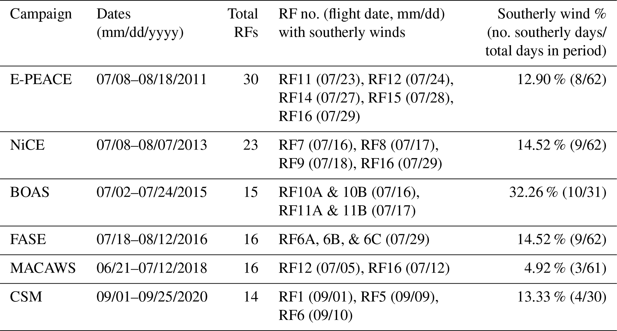
The goal of this study is to contrast aerosol and cloud characteristics between southerly and northerly flow regimes in the lower troposphere (below 3 km) offshore of central CA. Note that this study's primary objective is not to characterize meteorological and large-scale features associated with wind reversals, and we do not classify events based on whether they are CTDs but rather categorize events based on boundary layer wind direction. As a way to address the shortage of in situ observational data used for this research application, an important inventory is leveraged of airborne data that have been collected over the last 2 decades (Sorooshian et al., 2018) with increased sampling density of southerly flow cases relative to Juliano et al. (2019b). Such cases are difficult to sample owing to their lower frequencies (Table 1) compared to days with northerly flow and because aircraft flights do not occur each day, so some southerly cases are missed during airborne campaigns. In total, 17 d of data exist from Naval Postgraduate School (NPS) Twin Otter campaigns coinciding with southerly flow, with some days including multiple flights. One thing that has yet to happen in past studies is to use in situ data to compare more than just cloud water composition but also relevant variables such as aerosol number concentration (N_a) and N_d, which is crucial to intercompare with satellite data and put previous speculations about aerosol and cloud responses to southerly flow on sturdier ground. As the aircraft data are still limited, we complement the analysis with other datasets, including those from satellite remote sensors, models, and surface stations.

The structure of this paper is as follows: Sect. 2 reports on methods used; Sect. 3 shows results beginning with a discussion of how well a model can represent southerly winds, followed by assessing how well the datasets show more fine pollution during southerly days and if clouds respond accordingly with the usual chain of events associated with the Twomey effect (Twomey, 1974), whereby clouds have more but smaller drops at similar liquid water path; and Sect. 4 provides conclusions. The results of this work have implications for numerous societal and environmental factors sensitive to aerosol and cloud characteristics such as transportation (especially aviation), agriculture, biogeochemical cycling of nutrients and contaminants, and coastal ecology (Dadashazar et al., 2020).

2 Methods

This study relies on the use of multiple datasets to examine how aerosol and cloud characteristics vary between traditional northerly flow along the CA coastline compared to less common southerly flow periods. This study was initially inspired by airborne field measurements (Table 1) whereby on a few opportune flight days, southerly flow was encountered off the CA coast. Because these events were rare in comparison to the majority of flights with northerly flow (“Southerly wind %” in Table 1), data from several campaigns are compiled to increase the number data points for southerly flow days. The airborne data used here are all from summer periods, which is when most field studies have focused on this region to investigate aerosol–cloud interactions (e.g., Russell et al., 2013), allowing for easier intercomparison for interested readers. We enhance data volume by also conducting complementary analyses with data obtained from spaceborne remote sensing, surface-based stations, and models. Below we first describe the airborne datasets, followed by the wind classification method and then descriptions of the models, surface data, and satellite data.

2.1 Airborne field missions

This study utilizes data from six airborne missions based out of Marina, CA (white diamond; Fig. 1), using the Naval Postgraduate School (NPS) Twin Otter aircraft. Marina is approximately 5 km away from the coastline. The scientific target of these campaigns included a mix of aerosol–cloud interactions, aerosol microphysical processes, and characterization of wildfire emissions: the Eastern Pacific Emitted Aerosol Cloud Experiment (E-PEACE), the Nucleation in California Experiment (NiCE), the Biological and Oceanic Atmospheric Study (BOAS), the Fog and Stratocumulus Evolution Experiment (FASE), the Marine Aerosol Cloud And Wildfire Study (MACAWS), and the California Smoke Mission (CSM) (Table 1). Another Twin Otter mission from 2019 (Monterey Aerosol Research Campaign – MONARC) is not included in this analysis due to the lack of southerly flow days sampled during the campaign. The research flight (RF) paths for each campaign are shown in Fig. 1. In some instances, multiple flights were conducted on a single day, either to capture time-sensitive atmospheric features or to collect data beyond the endurance limit of the instrumented aircraft. For those days, RFs are assigned the same number but are distinguished with endings “A”, “B”, and “C” for successive flights, respectively. E-PEACE and NiCE had the most cases of southerly flow, partly owing to those campaigns having had the most flights: 5 out of 30 flights for E-PEACE and 4 out of 23 flights for NiCE. BOAS also had four flights with southerly flow (out of 15 flights), but they were spread across 2 flights days compared to E-PEACE and NiCE whose southerly flights were all on distinct days.

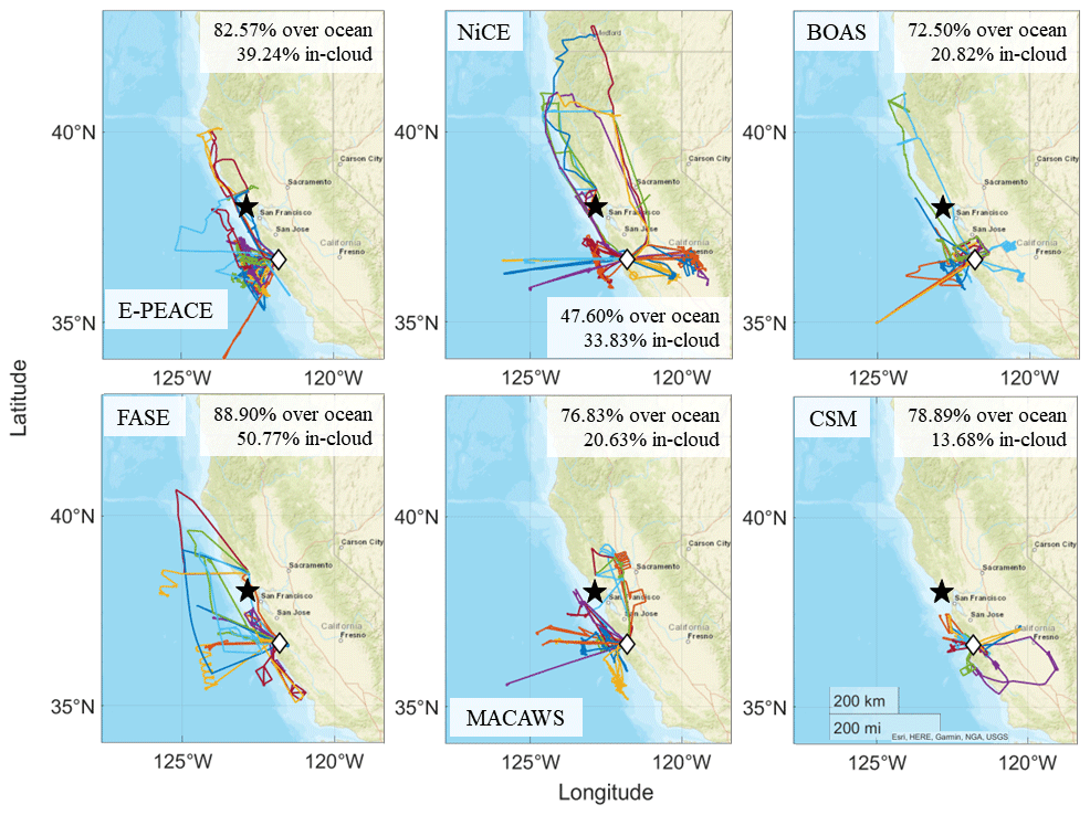
Figure 1 Research flight paths for the six Twin Otter campaigns used in this study. The aircraft base at Marina, CA, is denoted by a white diamond, and the IMPROVE station used in this study is indicated by a black star (Pt. Reyes National Seashore). The legends in each panel report the percentage of flight time spent over the ocean and in cloud over the ocean.

The Twin Otter flew at ∼ 55 m s⁻¹ and conducted measurements during level legs and sounding profiles over both the land and the ocean and within and above the boundary layer during flight periods ranging from 1 to 5 h. Additional information regarding aircraft and flight characteristics, as well as the general flight strategy, is summarized in Sorooshian et al. (2019). The general area of focus in this study was within the following range of coordinates, with many of the results specifically targeting just the ocean areas in this spatial domain: 35.31–40.99° N, 125.93–118.98° W.

This study's analysis focuses on maximizing the number of southerly and northerly cases available from the flight data rather than keeping a similar number of flights to represent southerly and northerly conditions. The rationale to include all available northerly flight days (which exceed southerly days; Table 1) is that their combined use is more representative of typical northerly conditions and less sensitive to inter-day variations. That being said, a random selection of northerly flight days was still used to compare to the more limited number of southerly flight days (not shown here), with the same general conclusions reached compared to using all northerly flight days.

Twin Otter instrumentation

Table 2 summarizes the relevant instruments used for each Twin Otter mission pertinent to this work. More extensive details about the instruments, and those not listed below such as relevant navigational and meteorological instruments, are described in Sorooshian et al. (2018).

Table 2 Summary of Twin Otter payload during the field campaigns used for this study. The six columns on the right show instrument availability for each campaign.

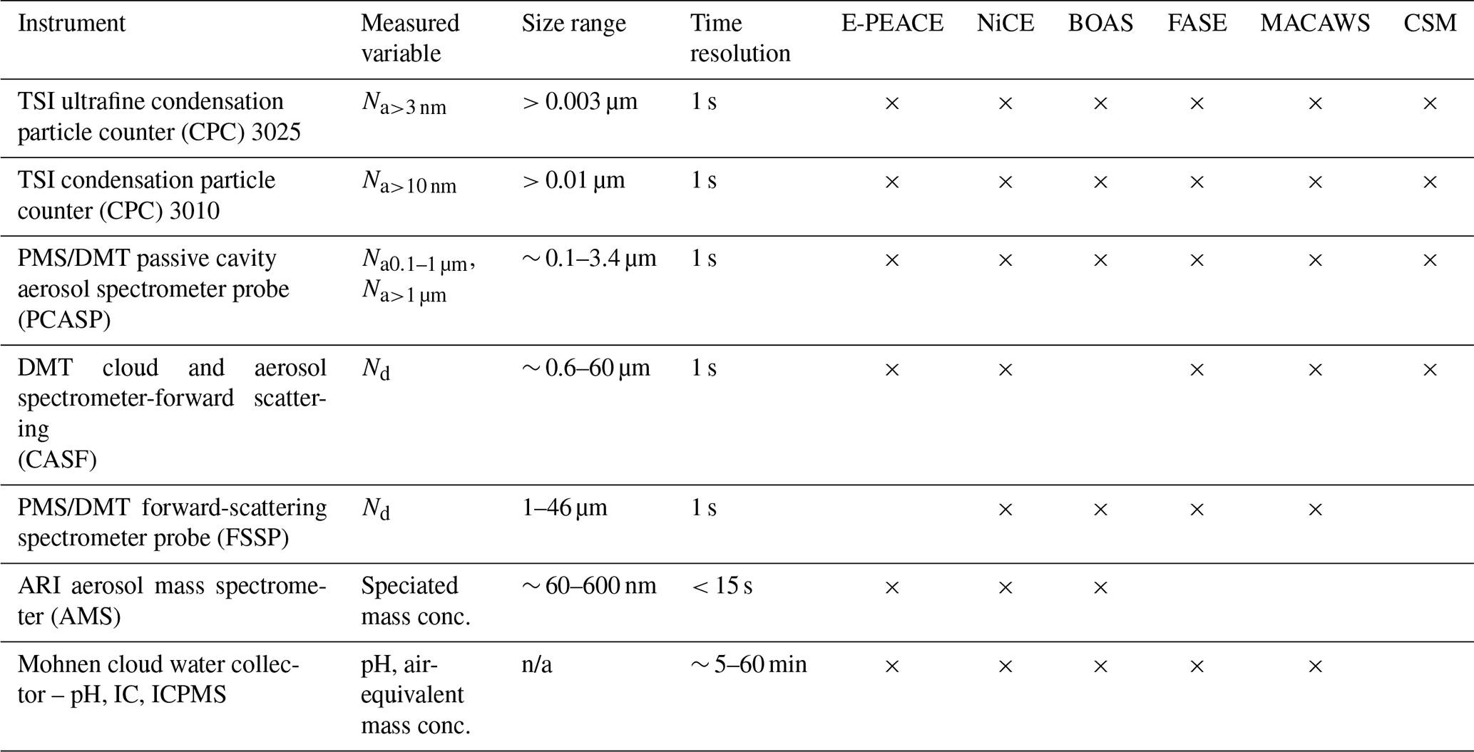
n/a: not applicable

Condensation particle counters (CPCs; TSI, Inc.) were used to measure particle number concentrations for diameters greater than 3 nm (N_a>3 nm or N_a3) and 10 nm (N_a>10 nm or N_a10), and a passive cavity aerosol spectrometer probe (PCASP; Particle Measuring Systems – PMS, Inc., modified by Droplet Measurement Technologies – DMT, Inc.) was used for diameters between ∼ 100 nm and 3.4 µm. The cloud and aerosol spectrometer-forward scattering (CASF; DMT, Inc.) measured the size distribution of larger particles and droplets between 0.6 and 60 µm for all missions except for BOAS when the forward-scattering spectrometer probe (FSSP; PMS, Inc., modified by DMT, Inc.) was used in its place. The cloud probes were calibrated before each field campaign to ensure consistency between the instruments (Sorooshian et al., 2018). The CASF and FSSP size distributions were integrated to determine total N_d and liquid water content (LWC) when the aircraft was in cloud using the criterion of LWC > 0.02 g m⁻³; all instances of LWC < 0.02 g m⁻³ were considered cloud-free and only considered for quantification of aerosol variables such as total N_a in different size ranges (Fig. S1 in the Supplement). Additionally, RFs categorized as southerly flow were filtered to only include data during periods when the horizontal wind direction was between 135 and 225°. A variety of statistics were calculated for the reported and derived variables (e.g., N_a>3 nm, N_a>10 nm, N_{a10–100 nm} (N_a>10 nm–N_{a0.1–1 µm}), N_{a0.1–1 µm}, N_a>1 µm, the ratio of N_a3 to N_a10 (N_a3 : N_a10), N_d, horizontal wind speed and direction) in categories of interest including medians and minimum and maximum values. The mode wind direction was calculated for each RF as well as each overall campaign, since that statistic is assumed here to be a better representation of typical wind directions rather than the median.

An aerosol mass spectrometer (AMS; Aerodyne Research Inc., ARI) was used during some campaigns to measure submicrometer (submicron) aerosol composition, specifically for non-refractory components (SO${}_{\mathrm{4}}^{\mathrm{2}-}$, NO${}_{\mathrm{3}}^{-}$, NH${}_{\mathrm{4}}^{+}$, Cl⁻, and organics). Coggon et al. (2012, 2014) discuss the AMS operational details and results in detail from some of the campaigns. Cloud water (CW) was collected using a Mohnen CW collector, which was manually placed above the fuselage of the Twin Otter during cloud penetrations for sample collection into vials kept inside the aircraft. After flights, samples were analyzed for pH and speciated concentrations of various water-soluble ions and elements, with a number of studies summarizing the operational details and selected results (e.g., Wang et al., 2014, 2016; MacDonald et al., 2018). An Oakton model 110 pH meter was used for E-PEACE, NiCE, and BOAS, and a Thermo Scientific Orion 8103BNUWP Ross Ultra semi-micro pH probe was used for FASE and MACAWS. Water-soluble ionic composition was measured via ion chromatography (IC; Thermo Scientific Dionex ICS – 2100 system), but some ions during E-PEACE, including Na⁺, could not be measured. Water-soluble elemental composition was measured via inductively coupled plasma mass spectrometry (ICP-MS; Agilent 7700 series) for E-PEACE, NiCE, and BOAS and via triple quadrupole inductively coupled plasma mass spectrometry (ICP-QQQ; Agilent 8800 series) for FASE and MACAWS. Cloud water was not collected during CSM. The IC species analyzed in this study are Cl⁻, NH${}_{\mathrm{4}}^{+}$, NO${}_{\mathrm{3}}^{-}$, non-sea-salt (nss) SO${}_{\mathrm{4}}^{\mathrm{2}-}$, and oxalate, and the ICPMS species analyzed are Ca²⁺, K⁺, Na⁺, and V. We used the following equation to calculate nss-SO${}_{\mathrm{4}}^{\mathrm{2}-}$ under the assumption that all Na⁺ is from sea salt (e.g., AzadiAghdam et al., 2019):

$$\begin{array}{}\text{(1)}& \left[\text{nss-}{\mathrm{SO}}_{\mathrm{4}}^{\mathrm{2}-}\right]=\left[{\mathrm{SO}}_{\mathrm{4}}^{\mathrm{2}-}\right]-\mathrm{0.253}\times \left[{\mathrm{Na}}^{+}\right].\end{array}$$

Aqueous concentrations of ions and elements were converted into air-equivalent concentrations using the mean LWC encountered when the aircraft was in cloud (LWC > 0.02 g m⁻³) during collection of individual samples.

Aircraft data were analyzed four different ways over the study domain. The primary focus of the analysis is using data within the spatial domain listed in Sect. 2.1 only when the aircraft was over the ocean (Fig. 1). In addition to an LWC maximum of 0.02 g m⁻³, another screening criterion was utilized to omit data during RFs strongly influenced by wildfire emissions (Table 3), which was when the median flight-wide N_a>10 nm value exceeded 7000 cm⁻³ for altitudes less than 800 m. This value was determined by closely examining flights that flew through areas with reported wildfire influence using flight notes. Data were alternatively analyzed for RF segments only over the ocean without the N_a>10 nm criterion applied and then also when the aircraft flew within the spatial domain over land and ocean both with and without the same wildfire criterion; those results are shown in Tables S1–S3. Note that CSM was the only campaign for which this criterion was not applied, as smoke was the sole focus of the mission and the flights are considered to all have been influenced to some extent. Moreover, CSM is unique amongst the campaigns examined where the scientific hypotheses to be tested are not as applicable due to the widespread smoke coverage, but we still examine it as it can provide useful insights.

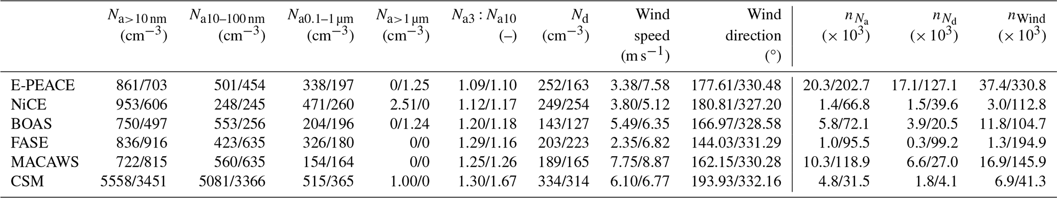
Table 3 Median values (southerly/northerly) of various parameters over the ocean with an N_a>10 nm filter such that RFs with median N_a>10 nm > 7000 cm⁻³ were removed from the final analysis to eliminate smoke interference. Mode values are used for wind direction. The instruments used for the parameters from left to right are as follows: CPC 3010, CPC 3010 – PCASP_<1 µm, PCASP_<1 µm, PCASP_>1 µm, CPC 3025, CPC 3010, and CASF. The right-hand columns indicate the number of data points used from each campaign, with $n_{N_{\mathrm{a}}}$ indicating the amount of data used for all N_a calculations; $n_{N_{\mathrm{d}}}$ is for cloud data, and n_Wind is for wind speed and direction. FSSP data were used for N_d only during BOAS, whereas CASF was used in other campaigns. These data are for the lowest 800 m above sea level. The reader is referred to Fig. S12 for box plots corresponding to the analysis in this table, as well as Table S4 for Mann–Whitney U-test p values.

Mann–Whitney U tests were performed for the aircraft data and the CW data, where the null hypothesis (p ≤ 0.05) was that the medians of certain variables (N_a, N_d, wind speed and direction) and species concentrations of southerly and northerly wind days were similar within a campaign.

2.2 Wind direction classification

To determine boundary layer wind direction in the study region, we used a number of data products, as each provided unique advantages related to either temporal, spatial, or vertical coverage. Data from the National Oceanic and Atmospheric Administration (NOAA) National Data Buoy Center (NDBC) were analyzed to verify the ocean surface wind direction was between 135 and 225°, which is considered southerly in this study. We focused on wind direction during 14:00–22:00 UTC to overlap with when the majority of RFs occurred (Marina, CA, is 7 h behind UTC). Other days classified as northerly flow adhered to surface wind direction between 315 and 45°. Five buoys were used to match the ones used in Juliano et al. (2019a): 46011 (Santa Maria: 34.94° N, 120.99° W), 46013 (Bodega Bay: 38.24° N, 123.32° W), 46014 (Point Arena: 39.23° N, 123.98° W), 46028 (Cape San Martin: 35.77° N, 121.90° W), and 46042 (Monterey: 36.79° N, 122.40° W). Buoy locations relative to the CA coast are shown in Fig. 1 of Juliano et al. (2019a).

The National Oceanic and Atmospheric Administration (NOAA) Hybrid Single-Particle Lagrangian Integrated Trajectory (HYSPLIT; Stein et al., 2015; Rolph et al., 2017) model was used to obtain back trajectories based on North American Mesoscale Forecast System (NAM) meteorological data (12 km resolution) ending at Marina, CA (36.67° N, 121.60° W; white diamond in Fig. 1), for 500, 900, 2500, and 4500 m a.g.l. Marina, CA, was selected as the ending point for the back trajectories as this was the takeoff and landing location for all six campaigns. These altitudes were selected to capture both marine boundary layer (MBL) and free-troposphere (FT) winds and reflect the variety of altitudes the Twin Otter aircraft flew at during the six campaigns in Table 1; however, the trajectories at 500 m were most important for connecting to the aircraft data analysis.

For Twin Otter flight days, aircraft wind data were used to confirm that wind direction was either southerly or northerly in the lowest 800 m of the flights (over ocean and land), which was the altitude range of most of the flight time. For a case-by-case basis, archived surface weather charts were accessed via the NOAA Weather Prediction Center (WPC) to investigate wind direction at specific sites (like Pt. Reyes).

We also used multi-channel RGB data from the Geostationary Operational Environmental Satellite-WEST Full Disk Cloud Product (GOES-15) to investigate cloud motion on northerly and southerly flow days. The analysis utilized time resolutions of every 3 h for E-PEACE; hourly for NiCE, BOAS, FASE, and MACAWS; and every half-hour for CSM. We investigated all days within a campaign month and not just days coinciding with an RF. For example, E-PEACE comprised flights from 9 July to 18 August 2011, and thus GOES data from 1 July through 31 August 2011 were investigated for that year. While not an exact tracer for air motion, we did observe that clouds tended to follow the prevalent air motion, particularly on southerly flow days.

2.3 NAAPS and COAMPS

Both the Navy Aerosol Analysis and Prediction System (NAAPS; Lynch et al., 2016; https://www.nrlmry.navy.mil/aerosol/, 24 June 2024) and the Coupled Ocean–Atmosphere Mesoscale Prediction System (COAMPS; Hodur, 1997) are used to support the analysis of airborne data collected during the six Twin Otter campaigns and assess how well they can simulate southerly flow on days when observational datasets indicate such flow directions offshore of CA. NAAPS is a global aerosol forecast model run by the US Naval Research Laboratory (NRL) in Monterey, CA, that predicts three-dimensional anthropogenic and biogenic fine (ABF), dust, sea salt, and biomass burning smoke particle concentrations in the atmosphere. NAAPS relies on meteorological data derived from the Navy Global Environmental Model (NAVGEM; Hogan et al., 2014) and considers 25 vertical levels in the troposphere. For this study, we utilized the reanalysis version of NAAPS (NAAPS-RA, hereafter called NAAPS) that assimilates aerosol depth observations to get a general sense of the simulated differences between southerly and northerly flow days for our region of focus and as a complement to the aircraft data.

The motivation for the usage of these models is twofold. The NAAPS-RA has a coarse horizontal resolution; however, it provides large-scale aerosol conditions with observational constraints on the model fields (i.e., incorporates satellite retrieved aerosol optical depth). It is important to have this relatively accurate large-scale aerosol background information for regional aerosol–cloud interaction research, as some of the background aerosol information (e.g., biomass burning smoke) and pollution are advected into the interested study area. Another minor reason is for model evaluation purposes: to see if models with different resolutions can resolve the studied phenomena, as this is less studied and is of interest to check if models have the capability to represent them. The use of NAAPS and COAMPS provides insight into how aerosol–cloud interactions from in situ data are represented by coarse-resolution models.

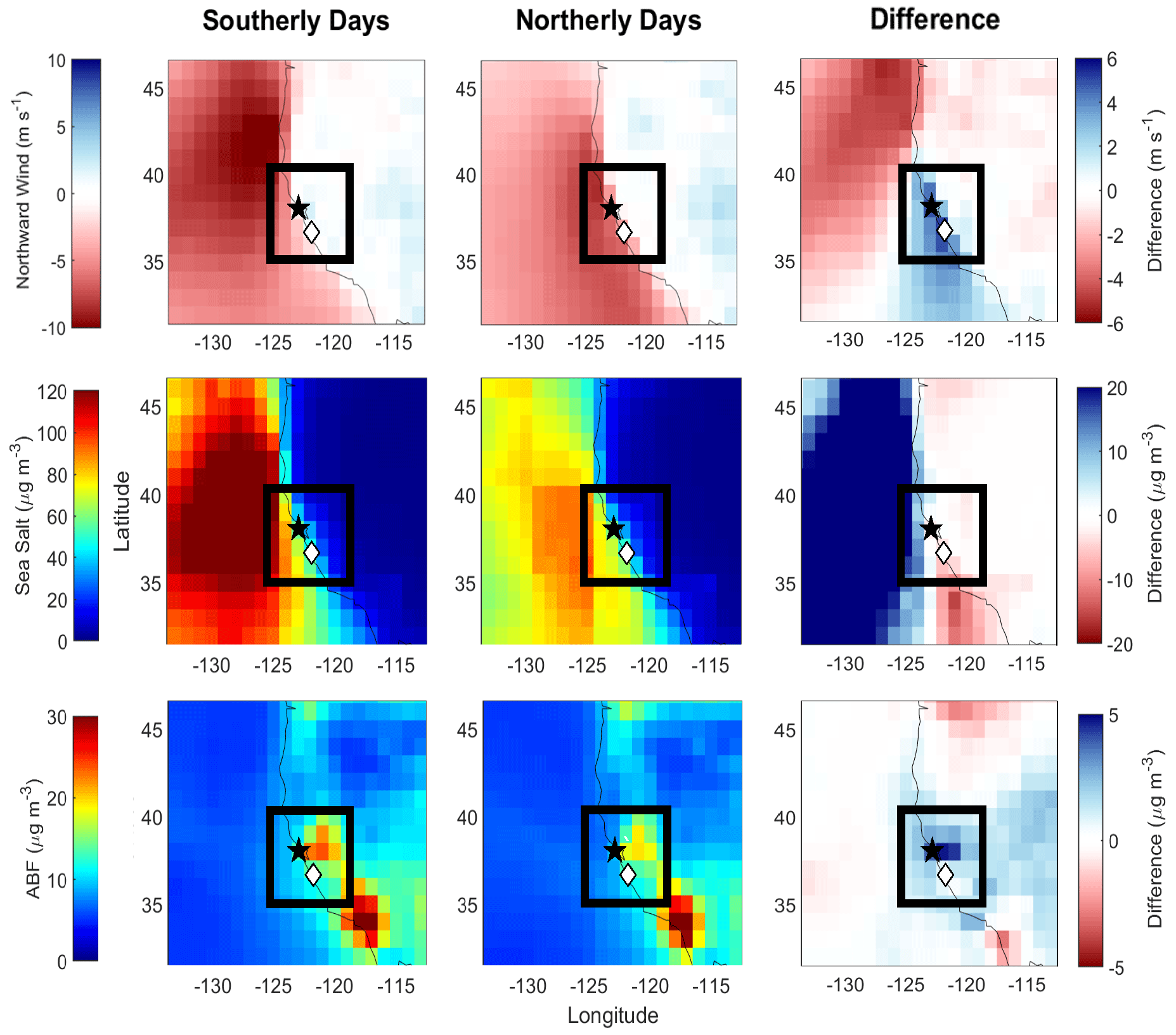
Figure 2 Average northward wind speed (v_wind; m s⁻¹), total sea salt mass concentration (µg m⁻³), and total ABF mass concentration (µg m⁻³) of campaign months at 18:00 UTC for the first through fifth NAAPS levels (up to ∼ 668 m above sea level) for southerly and northerly wind flow days. The rightmost panel illustrates the difference between southerly and northerly flow days. The air base in Marina, CA, is denoted by a white diamond, Pt. Reyes is indicated with a black star, and the black box indicates the region of focus in this study.

We investigated data for northward wind speed (v_wind, where northward, i.e., southerly, flow is indicated by positive values) and mass concentrations for ABF aerosols and sea salt (Fig. 2), along with smoke, dust, coarse aerosol, and fine aerosol (Fig. S2). Note that ABF represents secondarily formed species (SO${}_{\mathrm{4}}^{\mathrm{2}-}$ and secondary organic aerosol) and primary organic aerosol generally within the fine mode (< 1 µm). To be approximately similar to the average boundary layer height of all the missions used in this study, the first five vertical levels (max height of ∼ 668 m above sea level) of NAAPS were used for data analysis. Vertical profiles of temperature for each campaign categorized by flow regime are provided in Fig. S3 using aircraft data over the ocean to show the general structure of the lower troposphere in relation to the first five vertical levels of NAAPS.

For our analysis, the NAAPS data were first separated into southerly and northerly flow days for each campaign based on results from Sect. 2.2, and the average value of each parameter was calculated for four reported times: 00:00, 06:00, 12:00, and 18:00 UTC. The most focus is placed on 18:00 UTC, as that time coincided with most Twin Otter flight periods (results for the remaining time periods are in Figs. S4–S10). Then, all the parameters except v_wind were summed across the five vertical levels to get a total mass concentration (µg m⁻³) up to ∼ 668 m above sea level, whereas the average was calculated for v_wind. Those values were used to calculate the difference between southerly and northerly flow days at 1.0° × 1.0° spatial resolution.

COAMPS is a high-resolution meteorological forecast model developed by the NRL's Marine Meteorology Division (MMD) that outputs parameters like air temperature, winds, precipitation, cloud-base and cloud-top heights, and mass concentrations for the same aerosol species as those in NAAPS. For this study, we assessed the wind speed and direction as well as smoke from COAMPS and NAAPS for the purpose of contrasting with observational data. COAMPS maps were generated for this study by NRL at three different resolutions: 45, 15, and 5 km. To compare to NAAPS, 15 km resolution grids were used. To assess the efficacy of COAMPS and NAAPS at forecasting heavy pollution on a day with southerly winds, we performed a comparison of the two models for CSM RF6 at 18:00 UTC to match the flight time. The focus areas for both COAMPS and NAAPS matched that of the aircraft data mentioned in Sect. 2.1. The altitudes used for the COAMPS maps for wind speed and direction as well as smoke were 762 and 660 m, respectively, as the best match to the NAAPS maximum altitude used in this work.

2.4 IMPROVE

To investigate the difference in surface-level aerosol measurements between southerly and northerly flow days, this study utilized composition data from the Interagency Monitoring of Protected Visual Environments (IMPROVE) network (Malm et al., 1994; http://views.cira.colostate.edu/fed/, last access: 9 November 2023). Data were taken from the Pt. Reyes National Seashore surface station (38.07° N, 122.88° W) for the full campaign months shown in Table 1. Every third day, the gravimetric mass of particulate matter (PM_2.5 and PM₁₀) was measured. The PM_2.5 fraction was further analyzed via ion chromatography and X-ray fluorescence (XRF) for water-soluble ions and elements, respectively, along with organic and elemental carbon (OC and EC).

This study specifically investigated (µg m⁻³) PM_2.5, coarse mass (PM_coarse = PM₁₀ − PM_2.5), Cl⁻, NO${}_{\mathrm{3}}^{-}$, SO${}_{\mathrm{4}}^{\mathrm{2}-}$, Ni, K⁺, Si, V, EC, OC, and fine soil. The total OC measurement comes from a summation of four fractions of OC, which are categorized by a method of carbon analysis detection temperature (e.g., Chow et al., 1993; Watson et al., 1994). This method quantifies methane produced via volatilization of particulate species in pure helium at 120 °C (OC1), 250 °C (OC2), 450 °C (OC3), and 550 °C (OC4). Similarly, the total EC measurement is a summation of three fractions categorized via combustion temperatures in a 98 % pure helium and 2 % pure oxygen environment: 550 °C (EC1), 700 °C (EC2), and 800 °C (EC3). Fine soil concentrations are calculated as follows (Malm et al., 1994).

$$\begin{array}{}\text{(2)}& \begin{array}{rl}\mathrm{Fine}\mathrm{soil}\left(\mathrm{\mu }\mathrm{g}{\mathrm{m}}^{-\mathrm{3}}\right)& =\mathrm{2.2}\times \left[\mathrm{Al}\right]+\mathrm{2.49}\times \left[\mathrm{Si}\right]\\ & +\mathrm{1.63}\times \left[\mathrm{Ca}\right]+\mathrm{2.42}\times \left[\mathrm{Fe}\right]\\ & +\mathrm{1.94}\times \left[\mathrm{Ti}\right]\end{array}\end{array}$$

This equation was confirmed by several studies (e.g., Cahill et al., 1981; Pitchford et al., 1981; Malm et al., 1994) through comparisons of resuspended soils and ambient particles.

Upon examination, it was decided to only use data for E-PEACE and BOAS because those campaign periods had more than a single point with valid data for southerly days (three and two, respectively); recall that IMPROVE data are only available every third day due to the sample collection procedure, so some southerly days would not necessarily have available IMPROVE data. All the species analyzed had a status flag of V0 (“valid value”) or V6 (“valid value but qualified due to non-standard sampling conditions”), which are both considered valid data. We chose to include data flagged as V6 (Cl⁻, NO${}_{\mathrm{3}}^{-}$, and SO${}_{\mathrm{4}}^{\mathrm{2}-}$ for BOAS) due to the small quantity of usable data for southerly days. Additional information, like sampling protocols, is provided elsewhere (http://vista.cira.colostate.edu/Improve/sops/, last access: 9 November 2023). Like the aircraft and CW data, Mann–Whitney U tests were performed on this dataset to determine if the median species concentrations were equivalent for southerly and northerly days across a campaign.

2.5 MODIS

To assess cloud characteristics of southerly and northerly flow days during the campaign months of this study, we retrieved daily mean values within the same focus region defined for aircraft data in Sect. 2.1 (35.31–40.99° N, 125.93–118.98° W) for the following properties from the MODerate resolution Imaging Spectroradiometer (MODIS) on Aqua through NASA Giovanni (https://giovanni.gsfc.nasa.gov/giovanni/, last access: 9 November 2023): cloud effective particle radius (r_e; µm), cloud liquid water path (LWP; g m⁻²), cloud optical thickness (COT), cloud fraction (from cloud mask), and aerosol optical depth (AOD, combined dark target and deep blue at 0.55 µm for land and ocean). N_d (cm⁻³) was calculated from MODIS properties based on the following equation (Painemal and Zuidema, 2011).

$$\begin{array}{}\text{(3)}& N_{\mathrm{d}}=\mathrm{1.4067}\times {\mathrm{10}}^{-\mathrm{6}}\left[{\mathrm{cm}}^{-\mathrm{0.5}}\right]\times {\displaystyle \frac{{\mathrm{COT}}^{\mathrm{0.5}}}{r_{\mathrm{e}}^{\mathrm{2.5}}}}\end{array}$$

Additionally, retrieval data were only used when cloud fraction ≥ 30 % to maximize both data reliability and sample size (Mardi et al., 2021). The focus of the analysis is comparing median values of these remotely sensed variables between southerly and northerly days for E-PEACE and BOAS due to a similar LWP value for the two flow regimes (66.48 and 67.17 as well as 84.40 and 89.90 g m⁻², respectively). Data for the other campaigns are included in the Supplement. Additionally, this study used MODIS visible imagery on NASA Worldview to qualitatively identify smoke plumes, in addition to fire radiative power from the MODIS Fire Information for Resource Management System (FIRMS; https://earthdata.nasa.gov/firms, last access: 21 December 2023).

3 Results and discussion

3.1 Lower-tropospheric wind profile

We first examine NAAPS and airborne observations for the lower-tropospheric wind profile during the periods of analysis shown in Table 1. Note that the other datasets described in Sect. 2.2 are consistent with the airborne wind results and thus only NAAPS and aircraft data are discussed here for two reasons: NAAPS results are used to assess how such a model quantifies differences in winds between southerly and northerly flow days as identified with methods in Sect. 2.2, whereas aircraft data provide insight into typical wind speeds during southerly and northerly flow periods.

Beginning with the aircraft data, results are discussed here only for measurements over the ocean with the N_a>10 nm filter applied to remove smoke influence (Table 3). The mode of wind directions during southerly and northerly flow days in each campaign expectedly aligned with southerly (144–194°) and northerly flow (327–332°), respectively, because of how the classification was done (Sect. 2.2). Median wind speeds across each campaign ranged from 2.35–7.75 m s⁻¹ for southerly flow in contrast to 5.12–8.87 m s⁻¹ for northerly flow. This finding differs from what has been observed in previous studies, likely due to the difference in sampling location: aircraft observations from the surface to 800 m versus buoy and surface observations, respectively. All campaigns featured higher median wind speeds for northerly flow flights. However, when looking at the vertical wind profiles of each campaign for southerly and northerly flow days (Fig. S11), there were several instances where median wind speed at the surface for southerly flow days was greater than for northerly flow days. Both the median wind speeds and directions of southerly and northerly days were significantly distinct from one another for all of the studied campaigns (Table S4).

For context, boundary layer flow patterns from NAVGEM are provided in Fig. S13 for all southerly and northerly days at 18:00 UTC (Figs. S14 and S15 provide flow maps for each individual campaign). The average southerly flow pattern (Fig. S13a) captures generally weaker flow, particularly near Marina, CA, where a slight reversal can be observed. When looking at the flow maps for each campaign (Figs. S14 and S15), only BOAS and FASE captured a small wind reversal by Marina, CA, during southerly flow days. Both MACAWS and CSM had a circulatory pattern north of Marina, CA, near Pt. Reyes, and southerly flow is more clearly observed during the CSM campaign along the coast.

NAAPS values are discussed for v_wind for the lowest ∼ 668 m above sea level, with positive (negative) values representing southerly (northerly) flow (Fig. 2). This altitude range coincides with the airborne data shown in Table 3. The v_wind data are categorized into “southerly days”, “northerly days”, and “difference” (i.e., southerly – northerly values) for 18:00 UTC, which overlaps with most of the Twin Otter flight times (Fig. 1); results for 00:00, 06:00, and 12:00 UTC are provided in Fig. S4. Both southerly and northerly days had weaker v_wind closer to the coast (up to 35° N) compared to farther offshore over the ocean (∼ −3 and −9 as well as −4 and −6 m s⁻¹, respectively, for southerly and northerly flow). Slow, slightly northerly winds extended farther north to Marina and west to 123.5° W for southerly days, which is illustrated in red (differences exceeding ∼ 3 m s⁻¹ between flow regimes) in the “difference” panel. Northerly days also had an area of weaker v_wind north of 43.5° N, which is emphasized in the “difference” panel in blue (differences of −4 to −6 m s⁻¹). Generally, NAAPS was not able to fully capture southerly winds over the ocean and along the coast in that v_wind was not clearly positive (i.e., not northward); however, when looking at southerly flow for individual campaigns, NAAPS was sometimes able to capture areas with positive northward wind (i.e., southerly flow). When looking at the five vertical levels closest to the surface during periods when NAAPS was able to simulate positive northward winds, this feature was observed across all the levels, primarily along the coast near Marina, CA, or south of 34° N at 18:00 UTC, with lower wind speeds closer to the surface. Additionally, when looking at the averaged maps, the magnitude of the wind speed difference along the coastal area of the study domain appeared to align with the mechanics of coastal wind reversal and CTDs: the weakening of northerly wind and ultimate reversal of flow (e.g., Winant et al., 1987; Melton et al., 2009). A key conclusion from NAAPS is that the difference between southerly and northerly flow days matches expectations, with southerly days having a greater tendency towards higher v_wind compared to northerly days but, on average, still not necessarily distinctly positive v_wind values.

3.2 Aerosol response to southerly flow

3.2.1 Fire radiative power maps

Prior to discussing aerosol results, we address the influence of wildfire emissions, which is an aerosol source that varies in terms of strength between the six campaign periods in contrast to shipping and other forms of continental emissions that are more consistent from year to year. Past studies using airborne and surface-based data at Marina, CA (air base indicated by a white diamond in Figs. 1 and 2), overlapping with the six campaigns in Table 1 revealed the following in terms of notable biomass burning influence around Marina and offshore areas (e.g., Prabhakar et al., 2014; Braun et al., 2017; Mardi et al., 2018). (i) E-PEACE and BOAS showed no major influence of note. (ii) NiCE showed an influence around the last week of July 2013. (iii) FASE showed an influence between 25 July and 12 August. (iv) MACAWS showed a significant influence on flights during 28 June and 3 July owing to the aircraft having flown close to wildfire areas inland in northern CA. (v) CSM showed a significant influence throughout the campaign. These archived notes do not preclude the possibility of biomass burning influence during other periods of those campaigns as it relates to Twin Otter aerosol and cloud measurements.

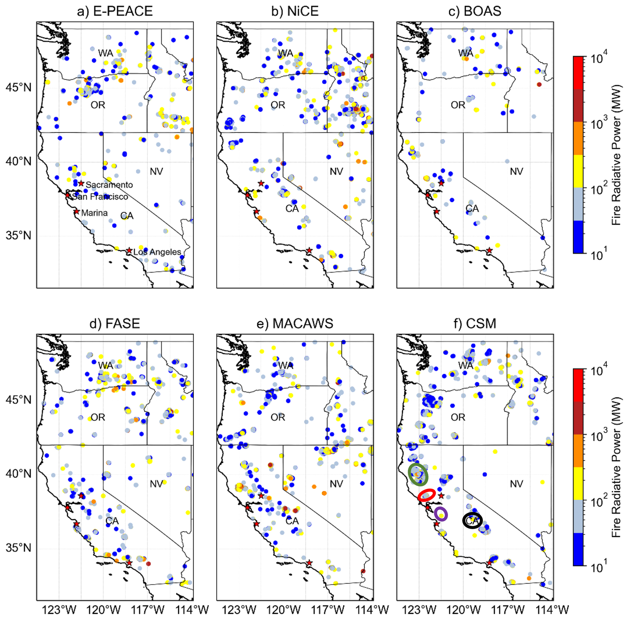
Figure 3 Spatial maps of fire radiative power (FRP), downloaded from the MODIS Fire Information for Resource Management System (FIRMS; https://earthdata.nasa.gov/firms) for the entire months spanning individual field campaigns in Table 1. Only FRP values with a high detection confidence level (≥ 80 %) are shown (Giglio et al., 2015). The circled areas in panel (f) correspond to some of the largest wildfires in CA state history that occurred in 2020 that are referred to in Sect. 3.4.2: August Complex fire (green), SCU Lightning Fire Complex (purple), Creek fire (black), and LNU Lightning Complex fire (red).

Spatial maps of fire radiative power (FRP; Fig. 3), indicative of burn intensity, show relatively less burning activity in immediate proximity to Marina during E-PEACE and BOAS. In contrast, the other campaigns show clusters of burning spots around Marina. Note that CSM, by virtue of its name, was focused largely on wildfires with dedicated RFs to sample smoke. MACAWS also was designed as a wildfire study but had fewer cases of strong plumes to sample, which included RFs on 28–29 June farther inland than most RFs, resulting in very high aerosol number concentrations (N_a>10 nm > 10 000 cm⁻³). These maps are mainly contextual to show the spatial distribution of fire sources, and specific conclusions cannot be gleaned solely based on these regarding which campaigns had more or less wildfire influence overlapping with the flight tracks. This is especially the case because smoke can be advected from distances far away from the study region. The wildfire filter described in Sect. 2.1 aims to filter out a large portion of smoke influence, at least at the regional level.

3.2.2 Fine aerosol

The first hypothesis of this study is that southerly flow yields higher fine-aerosol levels associated with anthropogenic and continental tracer species due to more perceived influence from land and shipping sources (Juliano et al., 2019a, b). This was also speculated by Hegg et al. (2008) although it was not examined in great detail by that study. Here we rely on results from a number of datasets including measurements from the Twin Otter (Tables 3 and 4) and the Pt. Reyes IMPROVE site (Fig. 4), along with NAAPS model results (Fig. 2).

Table 4 Median values (southerly/northerly) of water-soluble CW composition (µg m⁻³) over the entirety of three campaigns with sufficient data. The starred (^∗) values are reported in ng m⁻³. The number of samples used in each campaign is in the far right-hand column (n). The reader is referred to Table S5, which shows the p values from the Mann–Whitney U tests, as well as Fig. S16, which shows box plots of the CW composition results for the five campaigns with available data. Values shown as “–” denote when samples were below the limit of detection.

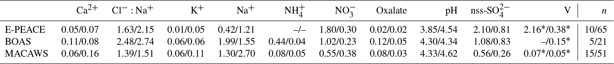
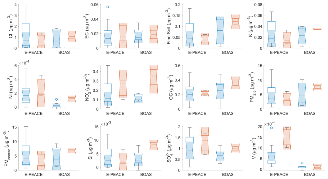
Figure 4 Box plots of IMPROVE data from the Pt. Reyes surface station. The southerly data for E-PEACE and BOAS (three and two points, respectively) are represented by the red boxes, and the northerly data (18 and 7, respectively) are represented by the blue boxes.

Airborne: particle concentration

Beginning with the Twin Otter data, aerosol data for 17 southerly flight days corresponding to 21 RFs are compared to 93 other flight days with predominantly northerly flow in Table 3 (box plots of the variables are in Fig. S12, and Mann–Whitney U-test results are in Table S4), as well as Tables S1–S3. We focus primarily on flight data over the ocean with the N_a>10 nm filter applied to omit wildfire influence; the other aircraft data result tables in the Supplement generally show the same trends as Table 3. We caution that the results of FASE, and to a slightly lesser extent NiCE, are not as meaningful as the other campaigns owing to the least amount of data for southerly conditions, with numbers of data points shown in the tables.

The total submicron aerosol number concentration, N_a>10 nm, was far larger for southerly flow (722–5558 cm⁻³) compared to northerly flow flights (497–3451 cm⁻³). Of the six campaigns, the only ones with higher median values in northerly flow were FASE and MACAWS, with small ΔN_a>10 nm of −80 cm and −93 cm⁻³, respectively. CSM exhibited the largest difference in median values for N_a>10 nm between southerly and northerly flow (ΔN_a>10 nm = 2107 cm⁻³), followed by NiCE (ΔN_a>10 nm = 347 cm⁻³) and BOAS (ΔN_a>10 nm = 253 cm⁻³). While these campaigns have a smaller relative sample size of southerly data ($n_{N_{\mathrm{a}}}$ < 6 × 10³; CSM: 4.8 × 10³, NiCE: 1.4 × 10³; BOAS: 5.8 × 10³), E-PEACE has a sizable amount of southerly data (20.3 × 10³) and the least fire influence of the missions included in this study, so we find it may be the most reliable campaign to analyze. There was a distinct difference between southerly and northerly days during E-PEACE as well, with ΔN_a>10 nm of 158 cm⁻³. As the number concentration in the submicron range dominates the total CPC concentrations, these results convincingly point to an enhancement of fine-aerosol pollution in southerly flow even without the N_a>10 nm filter (Table S1).

We examined various size ranges of particles in the submicron range as well. For particles between 10 and 100 nm, southerly conditions generally had higher number concentrations, again except for FASE and MACAWS and with more comparable levels during NiCE. As particles larger than 100 nm are more relevant for cloud condensation nuclei (CCN) activity, we also examined number concentrations for diameters between 0.1 and 1 µm, which show higher southerly levels except for MACAWS. Between campaigns, CSM overall exhibited the highest particle concentrations in this size range due to extensive wildfire emissions in the area, which are known to be linked with enhanced levels of particles larger than 100 nm in the same region (Mardi et al., 2018); this is why this campaign shows relatively large PCASP enhancements in both southerly and northerly flow conditions relative to the other campaigns (see in particular Tables S1–S2). Without the CPC filter (Table S1), only the medians for NiCE and BOAS on northerly wind days changed, resulting in the N_{a10–100 nm} median during NiCE being lower during southerly flow days compared to northerly days. When looking within the region of focus, the inclusion of land data in addition to ocean data (Tables S2–S3) leads to significant N_a differences (to a lesser extent for the filtered data; Table S3) compared to Table 3, including higher submicron concentrations for NiCE, BOAS, and FASE.

Although new particle formation (NPF) was not expected to be prominent in the lower 800 m owing mostly to high aerosol surface areas, especially due to sea spray emissions, we still examined the ratio of N_a above 3 nm relative to 10 nm (N_a3 : N_a10), as this ratio is a commonly used marker for identifying NPF. Such instances are more common in the free troposphere in the study region owing to reduced aerosol surface areas (Dadashazar et al., 2019). The results suggest that the N_a3 : N_a10 ratios for the two flow regimes were significantly different for all the campaigns except for MACAWS (higher ratios in southerly flow for BOAS and FASE), with median flow-direction-dependent values per campaign ranging from 1.09 to 1.30. During CSM, the median ratio value was 1.67 in northerly flow conditions due to presumed influence from high precursor levels in smoke plumes.

Airborne: tracer species in cloud water

We next turn to CW composition data (Table 4) to continue learning more about the effect of southerly flow and its associated emission sources. NiCE and FASE were not included in the CW calculations of Table 4 (but shown in Fig. S16) because there were fewer than five samples from RFs with southerly wind direction for those two campaigns, and CW was not collected during CSM. NO${}_{\mathrm{3}}^{-}$ and nss-SO${}_{\mathrm{4}}^{\mathrm{2}-}$, both representative of fine-aerosol pollution, were higher for southerly days, with a significant difference (Table S5) apparent in E-PEACE (1.80 and 0.30 as well as 2.10 and 0.81 µg m⁻³ for southerly and northerly days, respectively), as well as for NO${}_{\mathrm{3}}^{-}$ during BOAS (1.02 and 0.23 µg m⁻³ for southerly and northerly days, respectively). The same trend was observed for V (ship exhaust tracer) and NH${}_{\mathrm{4}}^{+}$, which can be used as a tracer for continental sources such as agriculture (Juliano et al., 2019b). Thus, these results help to provide more confidence in results from Juliano et al. (2019b) but with increased sampling across more campaigns. For E-PEACE and MACAWS, there were also lower southerly flow concentrations of K⁺ (0.01 and 0.05, 0.06 and 0.11 µg m⁻³) and Ca²⁺ (0.05 and 0.07, 0.06 and 0.16 µg m⁻³), suggestive of less influence from biomass burning and dust sources with the caveat that K⁺ and Ca²⁺ have sources other than biomass burning and dust.

There were also higher concentrations of oxalate during southerly days, which can be used as a tracer for aqueous processing (Hilario et al., 2021), wherein cloud droplets are formed from oxidized volatile organic compounds (Ervens et al., 2011; Ervens, 2015; McNeill, 2015). Further, there were significant differences in median concentrations between southerly and northerly flow days during BOAS and MACAWS (0.12 and 0.05 as well as 0.08 and 0.03 µg m⁻³, respectively). Precursors to oxalate are diverse including biogenic sources, biomass burning, combustion (e.g., Stahl et al., 2020, and references therein), and shipping, along with being associated with sea salt and dust owing to gas–particle partitioning (Sorooshian et al., 2013; Stahl et al., 2020; Hilario et al., 2021); such sources are presumed to be influential during southerly flow based on the notion that air masses are influenced by some combination of continental emissions and extended time in shipping lanes.

Cloud water pH was lower and thus more acidic on southerly days for all three campaigns (3.85 and 4.54, 4.30 and 4.34, 4.33 and 4.62 for southerly and northerly days during E-PEACE, BOAS, and MACAWS, respectively, and statistically different for E-PEACE and BOAS), which is another indicator of anthropogenic pollution enriched with acidic species (Pye et al., 2020). Increased acid levels can result in more Cl⁻ depletion when considering sea salt particles (e.g., Edwards et al., 2024, and references therein); interestingly, southerly days were characterized by lower Cl⁻ : Na⁺ ratios with median values of 1.39 (MACAWS), 1.63 (E-PEACE) (both campaigns for which southerly days were significantly different from northerly flow days), and 2.48 (BOAS), although the difference in MACAWS was only 0.12. Braun et al. (2017) noted that, theoretically, over 60 % of the Cl⁻ depletion in the submicron range could be attributed to nss-SO${}_{\mathrm{4}}^{\mathrm{2}-}$, and greater than 20 % in the supermicron range could be attributed to NO${}_{\mathrm{3}}^{-}$. As noted previously, nss-SO${}_{\mathrm{4}}^{\mathrm{2}-}$ and NO${}_{\mathrm{3}}^{-}$ were noticeably enhanced during southerly flow days, while the Cl⁻ : Na⁺ ratios were reduced. Schlosser et al. (2017) also reported that organic acids, notably oxalate, were significantly enhanced during periods of Cl⁻ depletion, which is reflected in our CW data. As E-PEACE was statistically the most robust dataset (and all CW species except Ca²⁺, NH${}_{\mathrm{4}}^{+}$, and oxalate had medians that were significantly different between southerly and northerly flow days), the results from CW convincingly align with more shipping and/or continental influence in southerly flow to impact cloud composition.

Surface: aerosol composition

We next examine surface composition data from the Pt. Reyes IMPROVE site. Mass concentrations of 12 PM composition variables were investigated to analyze important tracers along the coast (Fig. 4), with Mann–Whitney U-test p values for comparing southerly and northerly flow days shown in Table S6. It is important to recall that E-PEACE and BOAS were the only campaigns that had more than a single day of valid data coinciding with southerly flow because of the added challenge of IMPROVE sampling occurring every third day; therefore, northerly days had significantly more data points (18 for E-PEACE and 7 for BOAS) compared to southerly days (three and two, respectively). That is the general reason for the large whiskers on the box plots for northerly RFs during E-PEACE and the lack of whiskers for southerly RFs during BOAS. Another feature to note is the “folded-over” appearance of some of the box plots. This indicates a high variance within the dataset and a skewed distribution. We caution that this analysis is not very statistically robust owing to the rare nature of southerly days overlapping with IMPROVE sampling; however, we take a “better than nothing” approach to use in a supportive role in comparison to other datasets used to assess differences between southerly and northerly flow.

SO${}_{\mathrm{4}}^{\mathrm{2}-}$, NO${}_{\mathrm{3}}^{-}$, OC, V, Ni, and EC are reasonable tracer species representative of shipping and/or continental sources in the study region, as they have been utilized as tracers for these sources in previous studies (Wang et al., 2014; Maudlin et al., 2015; Wang et al., 2016; Dadashazar et al., 2019; Ma et al., 2019). These species were hypothesized to be more enhanced in the coastal CA zone on southerly flow days due to air spending time over shipping lanes and land upwind of the study region. Even with the limited southerly flow sample data, the results of Fig. 4 support this idea as southerly conditions coincide with higher median concentrations of these species than northerly days. The most striking relative differences were for NO${}_{\mathrm{3}}^{-}$ (southerly and northerly): 0.27 and 0.11 as well as 0.34 and 0.10 µg m⁻³ for E-PEACE and BOAS, respectively. NO${}_{\mathrm{3}}^{-}$ was the only species during BOAS that was found to have a median concentration that was statistically different between southerly and northerly days (Table S6). Ni and V are the primary trace metals in heavy-ship fuel oils and are commonly used as tracers for ship emissions (Celo et al., 2015; Corbin et al., 2018), and V was previously found enhanced in CW linked to ship emissions in E-PEACE (Coggon et al., 2012; Prabhakar et al., 2014). There were mostly higher concentrations of these species on southerly flow days (E-PEACE southerly and northerly: 0.20 and 0.17 as well as 1.56 and 0.58 ng m⁻³, respectively; BOAS southerly and northerly: 0.12 and 0.02 as well as 0.09 and 0.11 ng m⁻³, respectively), supporting the hypothesis of elevated shipping emissions. Also, a Mann–Whitney U test found that the median V concentrations during E-PEACE were statistically different for southerly and northerly days (Table S6).

Only BOAS exhibited higher PM_2.5 during southerly days compared to northerly days (7.61 and 4.82 µg m⁻³, respectively), with E-PEACE having roughly equivalent concentrations for the two flow regimes (3.39 and 3.78 µg m⁻³, respectively). This is likely due to how PM_2.5 is not the best marker for shipping and continental emissions owing to its inclusion of other species of marine and natural origin.

NAAPS: aerosol composition

To round out discussion of fine-aerosol pollution, we discuss NAAPS model results (Fig. 2). The largest enhancements in ABF mass concentrations occurred inland both north of Marina around Pt. Reyes and near the ports of Los Angeles and Long Beach. There was > 5 µg m⁻³ difference in ABF concentration between southerly and northerly days near Pt. Reyes. This suggests that while there were elevated levels of anthropogenic emissions in this area regardless of the flow regime, there were increased concentrations during southerly flow days according to NAAPS. An example HYSPLIT back trajectory for a southerly flow day (Fig. S17) shows air masses with likely influence from as far south as southern California and the US–Mexico border. Additionally, there is a strong ABF signal (> 30 µg m⁻³) around 34° N, 118° W for both categories of days, which is close to the ports of Los Angeles and Long Beach, two of the busiest container ports (in terms of cargo volume processed) in the United States and areas with elevated levels of NO_x and SO_x due to the ship exhaust and port emissions (Corbett and Fischbeck, 1997). As can be seen in the Fig. S6, the ABF concentrations around 34° N, 118° W and 38° N, 122° W increase throughout the day, with more significant increases north of the ports for southerly flow days. On southerly flow days, NAAPS results point to marked enhancements in fine-aerosol and smoke mass concentration north of Pt. Reyes over water but with mostly a reduction in such values to the south of Pt. Reyes over water. ABF represents the category of species that are most tied to the tracer species already shown to be enhanced in southerly flow, and thus at least this result from NAAPS is consistent with enhanced values across most of the study domain in southerly flow.

3.2.3 Supermicron aerosol

While this study hypothesizes that most of the aerosol changes in southerly flow will pertain to submicron aerosol, we still discuss supermicron aerosol characteristics to determine if there was any change observed. With all the complexities leading to sea salt emissions in the region (Schlosser et al., 2020), which is the predominant supermicron aerosol type in the study region's boundary layer, combined with the shifting wind directions and speeds leading up to and after a wind reversal (e.g., Juliano et al., 2019a), there was no underlying expectation for a change in concentrations during southerly flow events. Beginning with the aircraft observations, N_a>1 µm levels were generally low and usually zero in terms of flight median values simply due to so many zero values during an RF. Northerly flow conditions yielded median levels exceeding zero for E-PEACE (1.25 cm⁻³) and BOAS (1.24 cm⁻³). In contrast, southerly flow led to levels of 2.51 and 1.00 cm⁻³ during NiCE and CSM, respectively. The enhancement during southerly flow during at least CSM is presumed to be due to pervasive smoke during many of those RFs. However, the small median concentrations for each campaign make it hard to definitively determine if the lower concentrations during E-PEACE and BOAS were due to changes in flow regime or another factor. Figure S1 shows a scatterplot of total CASF number concentration versus effective diameter to separate out where cloud droplets are relative to probable sea salt particles and then coarse aerosol associated with the wildfires. There is considerable data coverage at LWC < 0.02 g m⁻³ for effective diameters below 5 µm and number concentrations exceeding 10 cm⁻³, with the latter surpassing what would be expected from sea salt (e.g., Gonzalez et al., 2022). It is very likely that dust particles can be entrained into regional smoke plumes as discussed in past work for the region (e.g., Maudlin et al., 2015; Schlosser et al., 2017). This will be discussed in more detail for a case flight demonstrating such high levels during southerly flow in Sect. 3.4.2.

Airborne CW results generally reveal no strong trends in either sea salt or dust tracer species between the flow regimes. The sea salt tracer species Na⁺ was lower for southerly days during E-PEACE (and statistically different) and MACAWS (0.42 and 1.21 as well as 1.30 and 2.70 µg m⁻³ for southerly and northerly days) but with an increase during BOAS (1.99 versus 1.55 µg m⁻³). The dust tracer species Ca²⁺ was, expectedly, much less abundant compared to Na⁺, without significant differences between flow regimes. However, as already noted (Sect. 3.2.2), the fine pollution in southerly flow likely still influenced supermicron aerosol characteristics via Cl⁻ depletion in salt particles.

In terms of IMPROVE data, PM_coarse, Si, fine soil, and Cl⁻ are the variables that would best coincide with typical sources of supermicron aerosol (i.e., dust and sea salt). They did not reveal any consistent trend for the two campaigns. Based on the lack of a general trend and reduced data for southerly flow days, it is concluded that there is insufficient evidence from IMPROVE to conclude that there is more or less dust or salt influence on southerly days.

The wind profile discussed in Sect. 3.1 has implications for sea salt aerosol production, which is influenced by wind speed. The breaking of wave crests to produce (mostly coarse-mode) spray droplets occurs at strong wind conditions (> 10 m s⁻¹) (Monahan et al., 1986). Additionally, jet droplets are produced via bubble bursting at lower wind speeds (> 5 m s⁻¹; Blanchard and Woodcock, 1957; Fitzgerald, 1991; Wu, 1992; Moorthy and Satheesh, 2000). On southerly days, there were faster northerly winds over the open ocean offshore west of 125° W, which corresponded to high sea salt concentrations (> 100 µg m⁻³) according to NAAPS, whereas northerly days had slower v_wind and less sea salt (65–90 µ g m⁻³) in those same areas farther offshore. In contrast, in the coastal areas south of 35° N, northerly days had higher sea salt concentrations (by 10–20 µg m⁻³) than southerly days with weaker (less negative) v_wind. NAAPS shows the same general trends for coarse aerosol mass compared to sea salt, with dust being far less abundant and more spatially heterogeneous in terms of enhancements and reductions between southerly and northerly conditions. In general, the NAAPS results are consistent with aircraft and IMPROVE results in that, in the study domain, there was not any pronounced difference in coarse aerosol characteristics during southerly flow. More research and data would be helpful, though, to put this conclusion on firmer ground.

3.3 Cloud responses

3.3.1 Airborne in situ results

As most campaigns exhibited higher N_a on southerly flight days, it matches expectation that most campaigns exhibited higher N_d values for southerly days (southerly and northerly values): E-PEACE (252 and 163 cm⁻³), BOAS (143 and 127 cm⁻³), MACAWS (189 and 165 cm⁻³), and CSM (334 and 314 cm⁻³). These campaigns had southerly N_d values that were ∼ 20 ± 4 cm⁻³ greater than the median values on northerly days, with a significant difference during E-PEACE (ΔN_d ∼ 89 cm⁻³). E-PEACE also had the most cloud data points compared to the other missions, qualifying it as the most robust campaign for inspection of cloud properties. The remaining two campaigns had the least amount of cloud data during southerly flow conditions (NiCE and FASE), and thus those results are of less importance to discuss. CSM had the highest N_d concentrations for both southerly and northerly days due to the strongest levels of pollution (from smoke) relative to the other campaigns.

3.3.2 Satellite data results

The second part of our hypothesis was that there would be a noticeable difference in cloud properties like N_d, r_e, and COT between southerly and northerly flow days (at fixed LWP), namely due to the change in emissions sources. In particular, we anticipated higher N_d and COT and lower r_e for southerly flow periods due to the Twomey effect (Twomey, 1974) and higher particle concentrations from continental pollution and shipping emissions. Six parameters were retrieved from MODIS, divided into southerly and northerly days for E-PEACE and BOAS, and visualized as box plots (Fig. 5). Cloud LWP medians for southerly and northerly days within E-PEACE (66.48 and 67.17 g m⁻²) and BOAS (84.40 and 89.90 g m⁻²) were not significantly different. Therefore, these two campaigns are the focus here, unlike the other campaigns that had larger differences (Table S7). The medians for N_d were higher for southerly days (138.54 and 91.99 as well as 96.59 and 72.80 cm⁻³ for southerly and northerly wind days during E-PEACE and BOAS, respectively), and the southerly and northerly medians during E-PEACE were significantly different from one another. Consistent with the Twomey effect (Twomey, 1974), the median r_e for southerly flow days was lower than northerly flow days (9.94 and 11.97 as well as 11.77 and 13.29 µm), with the medians during E-PEACE being significantly different. Cloud optical thickness was also higher for southerly days compared to northerly days for both campaigns (10.27 and 8.42 as well as 11.88 and 10.87 for E-PEACE and BOAS, respectively); however, the medians for each flow regime were not found to be significantly different from one another. We note that even for NiCE with LWP values being slightly higher for southerly days (82.78 g m⁻² versus 74.54 g m⁻²), the same general results are observed with southerly days having higher N_d and COT and reduced r_e (Table S7); the other three campaigns did not follow these N_d, COT, and r_e trends due to the larger LWP differences between flow regimes.

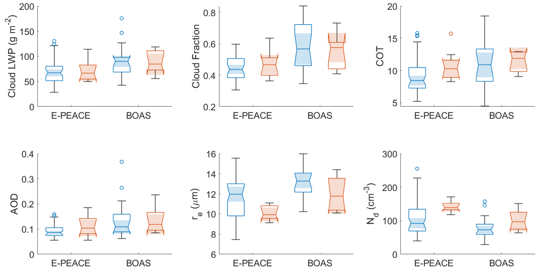
Figure 5 Box plots of MODIS data within the study region during the periods overlapping with E-PEACE and BOAS. The southerly data for E-PEACE and BOAS (eight points each) are represented by the red boxes, and the northerly data (44 and 17 points, respectively) are represented by the blue boxes. The notches (and shading, which helps to more clearly indicate where the notches end) of the boxes assist in the determination of significance between multiple medians. If the notches overlap, the medians are not significantly different from one another.

Although no differences were necessarily expected, we still examined cloud fraction and AOD, which were similar within a campaign for the two types of days (0.47 and 0.44 versus 0.58 and 0.57; 0.10 and 0.09 versus 0.12 and 0.11, respectively, for southerly and northerly wind days during E-PEACE versus BOAS). Based on these results, N_d, r_e, and COT differences between flow regimes match our hypothesis, and two out of the three parameters during E-PEACE were found to be significantly different between southerly and northerly days.

3.4 Case studies

In addition to looking at whole campaigns, we also looked closely at two RFs with southerly wind direction: NiCE RF16 (29 July 2013) and CSM RF6 (10 September 2020). NiCE RF16 was a unique flight, which coincided with a CTD event (Bond et al., 1996; Nuss, 2007), and its flight path extended past 125° W into a large stratocumulus cloud clearing (Crosbie et al., 2016; Dadashazar et al., 2020), which was unusual for the Twin Otter flights. CSM RF6 was on a heavily polluted day owing to biomass burning emissions during one of the worst wildfire periods in CA history. These case studies help emphasize the complexity of flow patterns in the region that influence the ability of aerosols from different sources to arrive at the boundary layer in the study region. The observed changes in aerosol and cloud properties between northerly and southerly days are likely not due to an instant switch in flow direction, but rather there is critical nuance in the timing, strength, and duration of the wind reversal, along with likely influence from free-tropospheric aerosol which can be sourced from various continental areas across California and even farther away (Dadashazar et al., 2019).

3.4.1 NiCE Research Flight 16

NiCE RF16 (29 July 2013) occurred on a day with a large stratocumulus cloud deck clearing, which, at its widest point, was 150 km (Crosbie et al., 2016). As noted in Crosbie et al. (2016), this was a CTD event during the time of the flight, and the boundary layer wind reversal (and resulting northwesterly flow) occurred under the stratocumulus cloud deck within 100 km of the coast (∼ 36.7° N, 123° W). The location of the wind reversal was known, which allowed us to investigate if there was any apparent gradient in aerosol and cloud variables from the coast to out over the ocean. The aircraft departed from Marina at approximately 17:00 UTC, with a nearly straight, westward path (Fig. 6a) toward the clear–cloudy boundary (the reader is referred to Fig. 1a of Crosbie et al., 2016, for the boundary location). At the clear–cloudy interface (∼ 36.7° N, 125° W, 18:45–20:00 UTC), stacked legs were performed at multiple levels in both the MBL and FT on both sides of the boundary. Subsequently, the aircraft returned to Marina following the initial outbound path. To visualize the location and general timing of the wind reversal (Fig. 6b–c), 48 h back trajectories from HYSPLIT were used. This contrasts with the 24 h back trajectories used to confirm southerly wind flow in Sect. 2.2. For the case studies, 48 h periods were used to have a better understanding of air mass history. This case of southerly wind is one where the sampled air mass was likely to have spent more time in the coastal area just south of Marina compared to traditional northerly flow, where there was a presumed influence from shipping emissions and possibly advected continental air.

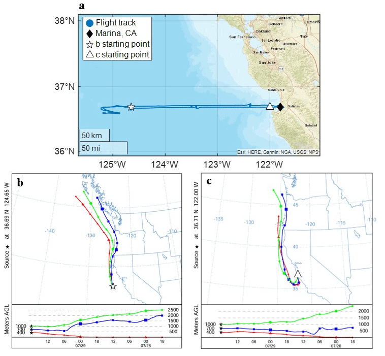
Figure 6 (a) NiCE RF16 (29 July 2013) flight track, with Marina represented by a solid black diamond, the starting point of the HYSPLIT back trajectory in panel (b) indicated by a white star, and the starting point of the HYSPLIT back trajectory in panel (c) indicated by a white triangle. (b) 48 h back trajectory of a point (36.69° N, 124.65° W) along the flight path outside of the southerly wind zone (HYSPLIT end time: 18:00 UTC). (c) 48 h back trajectory of a point (36.71° N, 122.00° W) along the flight path at the beginning of the RF (HYSPLIT end time: 17:00 UTC) where there was southerly flow. Panels (b) and (c) detail back trajectories for three different altitudes: 400, 700, and 1000 m.

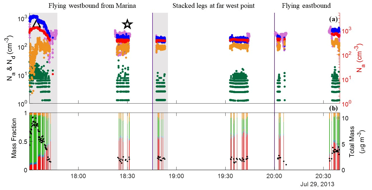
Figure 7 Data from NiCE RF16 in the MBL (< 525 m). The gray shading indicates time periods with mostly southerly winds, and the purple lines across all graphs indicate flight zones (outbound track, stacked legs at the farthest west point, and inbound track). (a) The colored points on the left-hand axis correspond to N_{a0.1–1 µm} (blue, PCASP_<1 µm), N_a>1 µm (green, PCASP_>1 µm), and N_d (light purple, CASF). The colored points on the right-hand axis correspond to N_a>10 nm (red, CPC) and N_{a10–100 nm} (yellow, CPC 3010 – PCASP_<1 µm). The triangle corresponds to the HYSPLIT back-trajectory end point seen in Fig. 6c, and the star corresponds to the HYSPLIT back-trajectory end point seen in Fig. 6b. (b) Stacked bar plot of AMS mass fractions of SO${}_{\mathrm{4}}^{\mathrm{2}-}$ (red), NO${}_{\mathrm{3}}^{-}$ (blue), organics (green), and NH${}_{\mathrm{4}}^{+}$ (orange), overlaid with total mass concentration (µg m⁻³; black).

We investigated gradients from the coast to farther offshore including past the wind reversal for several parameters, including N_a, N_d, and AMS total mass and mass fractions in both the sub-cloud MBL (< 525 m a.g.l., Fig. 7) and the FT (> 765 m a.g.l., Fig. S18); the altitudes of both were defined in Crosbie et al. (2016). There was a general trend of decreasing number concentration, especially for N_{a0.1–1 µm}, N_a>10 nm, and N_d, from the coast to slightly before the stacked legs at the far west point (1245 and 189, 1240 and 390, and 772 and 263 cm⁻³, respectively, at ∼ 17:32 and 18:30 UTC). There was a wide range of supermicron concentrations for the whole flight duration; however, generally, there was a slight decrease in N_a>1 µm along the flight path going west as well, but it was not as pronounced as the other variables (24 and 4 cm⁻³).

The eastbound leg to Marina was an interesting situation as there was no longer southerly flow closer to the coast, yet there was still a concentration increase for number and cloud drop concentrations but not up to the same maximum levels that were observed on the westbound portion of the flight, probably owing to the reduced influence from areas south of the sampling area (N_{a0.1–1 µm}: 248 and 435, N_a>10 nm: 454 and 752, N_d: 272 and 434, and N_a>1 µm: 5 and 19 cm⁻³ for eastbound and westbound legs at ∼ 20:00 and 20:37 UTC). AMS mass concentrations dropped significantly in the outbound portion of the flight, from total mass as high as 10.16 µg m⁻³ (∼ 17:30 UTC) to 1.55 µ g m⁻³ (∼ 17:45 UTC), the latter of which was approximately 10 km offshore. During that period, the organic mass fraction decreased from 0.81 to 0.28 in favor of growing SO${}_{\mathrm{4}}^{\mathrm{2}-}$ mass fraction from 0.11 to 0.50. On the inbound track, similar to $N_{\mathrm{a}}/N_{\mathrm{d}}$ results, there was not as much of an enhancement in total mass (max of 4.41 µg m⁻³ at ∼ 20:40 UTC) and the chemical profile revealed more comparable levels of SO${}_{\mathrm{4}}^{\mathrm{2}-}$ and organic mass fractions (0.39 and 0.52, respectively, at ∼ 20:40 UTC) in contrast to the outbound track that showed a higher organic mass fraction right by the coast.

The results suggest that the enhanced residence time of air masses (due to the wind reversal) in an area with a presumed influence from shipping emissions (see Fig. 9 in Coggon et al., 2012) and continental pollution yielded an offshore gradient in N_a, N_d, and aerosol composition. Also, the results help show that this general coastal zone area in the location of the wind reversal is enhanced with fine pollution, which will generally affect aerosol and cloud characteristics if air masses spend prolonged time in it during southerly flow conditions. This all being said, it is hard to unambiguously attribute the aerosol and cloud changes to emissions from a particular area and source due to the complex flow nature in both the horizontal and vertical directions during the wind reversal period. This case study helps motivate continued research studying these events.

The trends in the FT are much more ambiguous than those in the MBL (Fig. S18). Similar to the MBL, there was a decrease in N_{a0.1–1 µm} and N_a>10 nm from the coast to near the stacked legs (2467 and 395 as well as 2820 and 689 cm⁻³, respectively, at ∼ 17:26 and 18:44 UTC); however, there was no discernable trend for N_a>1 µm. There were no apparent offshore trends for AMS total mass or speciated mass fractions. Additionally, on the eastbound flight leg, there was not a clear trend for any of the parameters. This suggests that the effects of the southerly winds were stronger in the MBL than the FT.

3.4.2 CSM Research Flight 6

CSM stands out among all of the examined campaigns owing to the strength and temporal persistence of wildfire plumes, which was also the main focus of the mission. Of the top 3 % (n = 12) of the largest fires in CA in the historical record, four occurred in 2020 (circled in Fig. 3): the August Complex fire (16 August, Mendocino County), the SCU Lightning Fire Complex (18 August, Santa Clara County), the Creek fire (4 September, Madera County), and the LNU Lightning Complex fire (16 August, Hapa County) (Keeley and Syphard, 2021). These four fires were a mix of both merged (August Complex) and unmerged (LNU Lightning Complex) fires that burned over 417, 160, 153, and 146 kha, respectively, and burned for months after they were ignited.

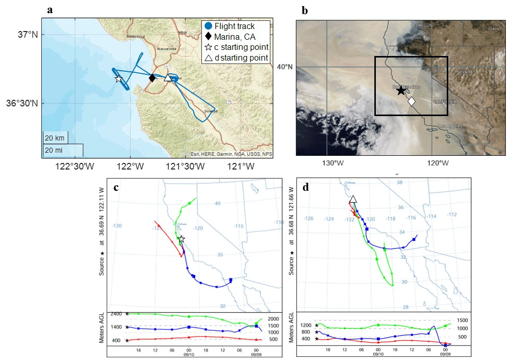
Figure 8 (a) CSM RF6 (10 September 2020) flight track, with Marina, CA, represented by a solid black diamond, the starting point of the HYSPLIT back trajectory in panel (c) indicated by a white star, and the starting point of the HYSPLIT back trajectory in panel (d) indicated by a white triangle. (b) NASA Worldview image, with Marina, CA, represented by a white diamond and Pt. Reyes denoted by a black star. (c) 48 h back trajectory of a point (36.69° N, 122.11° W) along the flight path during the sounding over Monterey Bay (HYSPLIT end time: 21:00 UTC) at three different altitudes: 400, 1400, and 2400 m. (b) 48 h back trajectory of a point (36.68° N, 121.66° W) along the flight path during the sounding over Salinas (HYSPLIT end time: 19:00 UTC) at three different altitudes: 400, 800, and 1200 m. Panels (c) and (d) utilized different altitudes for the back trajectories to reflect the different maximum altitudes of the two major soundings of the flight.

CSM RF6 (10 September 2020) included two major components (Fig. 8a): a spiral over Salinas (max altitude of 6172 m at ∼ 20:00 UTC) and a spiral over Monterey Bay (max altitude of 4822 m at ∼ 21:70​​​​​​​ UTC). The entire region was heavily impacted by smoke during CSM RF6 (Fig. 8b). Additionally, around 36.5° N, 125° W, there is an area not dominated by smoke but rather clouds, pointing to the likelihood of smoke–cloud interactions in the region on not just this day but other CSM days with similar smoky conditions. HYSPLIT back trajectories for the two spirals for a 48 h period were generated (Fig. 8c and d). For the spiral over Monterey Bay (Fig. 8c), the lowest-altitude trajectory (trajectory beginning at 400 m) is mostly northwesterly, the second-lowest altitude (trajectory beginning at 1400 m) is primarily southerly, and the highest altitude (trajectory beginning at 2400 m) is approximately northeasterly. The highest-altitude back trajectory passes over the LNU Lightning Complex fire (red oval; circled in Fig. 3). For the spiral over Salinas (Fig. 8d), all three altitude levels (400, 800, and 1200 m a.g.l.) reveal southerly trajectory paths, and the air masses from the second-highest-altitude back trajectory possibly had some influence from the SCU Lightning Fire Complex (purple oval) and the August Complex fire (green oval) due to offshore and northerly flow in the preceding 36 h (Fig. 3).

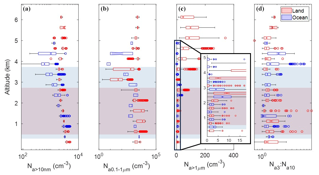
Figure 9 CSM RF6 box plot vertical profiles of (a) N_a>10 nm (cm⁻³), (b) N_{a0.1–1 µm} (cm⁻³; PCASP_<1 µm), (c) N_a>1 µm (cm⁻³; PCASP_>1 µm), and (d) N_a3 : N_a10. Data are shown every 500 m over land (red) and ocean (blue) above the MBL, which is the maximum altitude of the first bins for all the panels. Panel (c) has an additional focus on altitudes ≤ 5 km (N_a>1 µm ≤ 18 cm⁻³). The red and blue shading indicates altitudes over the land and ocean, respectively, with southerly winds.

The vertical profiles of temperature, wind speed, and wind direction are provided in Fig. S19 for context. Notably, the vertical region with southerly flow was thicker over the ocean (approximately 370–3700 m) versus over land (540–2900 m). N_a for different size ranges and N_a3 : N_a10 are shown separately for land and over the ocean (Fig. 9). There was more variability in N_a>10 nm (Fig. 9a) over the ocean, with a general decrease in concentration with an increase in altitude for data over both land and ocean, followed by increasing N_a>10 nm above the region of primarily southerly flow (non-shaded points). As illustrated by the composite boundary layer flow pattern in Fig. S15e–f, smoke along the coast during southerly flow periods was re-circulated northwest of Marina, CA, near the flight path (which was not observed for the northerly composite flow pattern), which could have also influenced the elevated aerosol concentrations during this flight. There was not much change in N_a>1 µm (medians 1–3 cm⁻³; range 0–6 cm⁻³; Fig. 9c) until > 2.5 km, where concentration increases over land (medians 5–97 cm⁻³; range 0–297 cm⁻³) where there is primarily northerly flow, likely from sampling smoke plumes. Over the ocean, low supermicron particle concentrations are observed (≤ 7 cm⁻³). These results show that during extensive smoky periods, the flow regime does not matter in cases like RF6 due to smoke generally being all across the region. Furthermore, the results show that supermicron particle concentrations are certainly enhanced in smoke plumes, as has been observed before in the study region (Mardi et al., 2018) but not to this pronounced extent, especially at high altitudes over land.

The N_a3 : N_a10 ratio (Fig. 9d) was generally consistent over land across all vertical levels, with a good number of outliers in the region of primarily southerly flow. The medians of the ratios over the ocean were usually lower than the medians over land until 3.5 km. There was no discernable difference in the N_a3 : N_a10 ratio over land between southerly and northerly flow (medians approximately 1.35 until > 5.5 km) or over the ocean (medians for both flow regimes approximately 1.20, with a slight bump to 1.26 and 2.14 between 3.5 and 4.5 km). The reader is referred to Sect. S1 (Supplement) for a discussion about NAAPS and COAMPS results for this case study as they relate to flow behavior and aerosol characteristics.

4 Conclusions

In this study, we utilized multiple types of data, including a large repository of NPS Twin Otter data, to compare coastal aerosol and cloud characteristics near central CA for northerly and southerly wind regimes in the lower troposphere. Juliano et al. (2019a) previously called for future studies to utilize in situ observations to support their investigation into cloud properties using satellite observations. Our study is among the first to investigate aerosol and cloud droplet number concentrations through in situ aircraft data in addition to CW composition and intercompare those results with satellite data, as well as models and surface station data. This builds upon previous studies, such as Juliano et al. (2019b), by utilizing similar data sources across a broader range of sources.

We find strong support for our first hypotheses that more fine-aerosol pollution is present off the CA coast during southerly flow due to a likely influence from shipping exhaust and continental emissions. We caution that there is considerable complexity in flow patterns both horizontally and vertically when northerly winds change to southerly winds, and this warrants more research to study, for instance, how influential free-tropospheric air is for the boundary layer aerosol changes occurring on southerly flow days. Submicron aerosol pollution is found to be higher during southerly flow days (particularly during E-PEACE) with respect to both N_a (N_a>10 nm, N_{a10–100 nm}, N_{a0.1–1 µm}) and concentrations of shipping and continental tracer species in surface data (SO${}_{\mathrm{4}}^{\mathrm{2}-}$, NO${}_{\mathrm{3}}^{-}$, OC, V, Ni, and EC) and CW samples (nss-SO${}_{\mathrm{4}}^{\mathrm{2}-}$, NO${}_{\mathrm{3}}^{-}$, NH${}_{\mathrm{4}}^{+}$, V, and oxalate). Cloud water is shown to be more acidic during southerly flow along with more Cl⁻ depletion based on lower Cl⁻ : Na⁺ ratios. A secondary hypothesis was that increased influence from shipping and/or continental emissions would lead to enhanced N_d and COT and lower r_e (at fixed LWP) due to the Twomey effect (Twomey, 1974). Both the airborne in situ data and satellite retrievals show increased N_d on southerly days. The satellite retrieval data also reveal higher COT and lower r_e during southerly flow. The increase in N_d and decrease in r_e associated with the northerly to southerly reversal match results of a previous study in the region (Juliano et al., 2019a). The analysis of CSM RF6 reveals that during heavy biomass burning periods with prevailing smoke, there is relatively no difference in aerosol or cloud properties associated with changes in flow regime. Based on the NAAPS evaluation, while coarse-gridded models can capture differences in wind direction and aerosol concentration between southerly and northerly flow days, they are not fully able to reproduce southerly flow. During cases when there was known southerly wind, NAAPS was only sometimes able to represent it, which is a topic encouraged for pursuit in future work.

A limitation in this type of study to address in the future is the difficulty of obtaining detailed in situ data during southerly wind conditions. As already noted, wind reversals along coasts extend to a number of other global regions (e.g., South America, southern Africa, Australia) and thus it is recommended to continue increasing the sample data volume to better understand changes in aerosol and cloud properties as a function of wind direction along coastal regions. Intercomparisons with models, as partly done here, can aid in determining if model resolution should improve to better simulate these events. Generally speaking, the prevalence of fine aerosol on southerly flow days and associated changes in cloud microphysical properties are important findings with implications for weather, health, coastal ecology, and aviation.