the Creative Commons Attribution 4.0 License.
the Creative Commons Attribution 4.0 License.
 | 24 Jul 2024
Revising VOC emissions speciation improves the simulation of global background ethane and propane
Matthew J. Rowlinson
Mat J. Evans
Lucy J. Carpenter
Katie A. Read
Shalini Punjabi
Adedayo Adedeji
Luke Fakes
Ally Lewis
Ben Richmond
Neil Passant
Tim Murrells
Barron Henderson
Kelvin H. Bates
Detlev Helmig
Non-methane volatile organic compounds (NMVOCs) generate ozone (O3) when they are oxidised in the presence of oxides of nitrogen, modulate the oxidative capacity of the atmosphere and can lead to the formation of aerosol. Here, we assess the capability of a chemical transport model (GEOS-Chem) to simulate NMVOC concentrations by comparing ethane, propane and higher-alkane observations in remote regions from the NOAA flask Network and the World Meteorological Organization's Global Atmosphere Watch (GAW) network. Using the Community Emissions Data System (CEDS) inventory, we find a significant underestimate in the simulated concentration of both ethane (35 %) and propane (64 %), consistent with previous studies. We run a new simulation in which the total mass of anthropogenic NMVOC emitted in a grid box is the same as that used in CEDS but with the NMVOC speciation derived from regional inventories. For US emissions, we use the National Emissions Inventory (NEI); for Europe, we use the UK National Atmospheric Emissions Inventory (NAEI); and for China, we use the Multi-resolution Emission Inventory model for Climate and air pollution research (MEIC). These changes lead to a large increase in the modelled concentrations of ethane, improving the mean model bias from −35 % to −4 %. Simulated propane also improves (from −64 % to −48 % mean model bias), but there remains a substantial model underestimate. There were relatively minor changes to other NMVOCs. The low bias in simulated global ethane concentration is essentially removed, resolving one long-term issue in global simulations. Propane concentrations are improved but remain significantly underestimated, suggesting the potential for a missing global propane source. The change in the NMVOC emission speciation results in only minor changes in tropospheric O3 and OH concentrations.
- Article
(19354 KB) - Full-text XML
- BibTeX
- EndNote


Volatile organic compounds (VOCs) play a central role in the chemistry of the atmosphere. Methane dominates much of this chemistry, due to its large emissions from both natural and anthropogenic activities (Kirschke et al., 2013), while a comparable mass of isoprene (C5H8) is also emitted globally by the biosphere (Guenther et al., 1995). However, other non-methane volatile organic compounds (NMVOCs) such as alkanes, alkenes, aromatics, alcohols and carbonyls are also emitted into the atmosphere by both natural and anthropogenic processes (Simpson et al., 1999; Li et al., 2017b; Hoesly et al., 2018). Following oxidation, NMVOCs contribute to the formation of tropospheric ozone (O3), a pollutant with detrimental effects on both climate and human health (Monks et al., 2015; Szopa et al., 2021), and impact the global oxidative capacity through changes to the OH concentration (Fry et al., 2012). Some NMVOCs also contribute to the production of secondary organic aerosols (Hodzic et al., 2016).
Ethane and propane are two of the most globally abundant NMVOCs. Atmospheric concentrations and trends in ethane and propane are controlled by the balance of their emissions, which are predominantly anthropogenic (Aydin et al., 2011; Simpson et al., 2012; Helmig et al., 2014), and their major loss by reaction with the OH radical. Previous modelling studies have underestimated the atmospheric concentrations of ethane and propane by as much as a factor of 2 for ethane, and perform even worse for propane (Pozzer et al., 2007; Dalsøren et al., 2018; Emmons et al., 2015). As there is no secondary chemical production of ethane and propane, the low bias must be the result of underestimated emissions or an overactive sink. Previous studies have concluded that the underestimate is primarily due to an underestimate in anthropogenic emissions inventories (Carmichael et al., 2003; Pozzer et al., 2007; Tzompa-Sosa et al., 2017; Dalsøren et al., 2018; Emmons et al., 2015). Possible explanations for this underestimate range from missing natural emissions sources (Etiope and Ciccioli, 2009; Dalsøren et al., 2018), a misrepresentation of the rapid increases in industrial emissions (Franco et al., 2016) and/or broad underestimates in bottom-up anthropogenic inventories (Pozzer et al., 2010; Dalsøren et al., 2018). Emissions inventories have a number of uses, from regulatory compliance to use in chemical and climate modelling. The latter can be used in the assessment of the air quality or climate policies. Priority is often given to species with a direct impact on air quality (NOx and SO2) or to greenhouse gases (CO2 and CH4) rather than species such as NMVOCs which are often seen as being of secondary importance. Global inventories, such as the Community Emissions Data System (CEDS) (Hoesly et al., 2018) aggregate local, country-based emission estimates where available to build a global emission data set based on the best estimates from regional data. The CEDS emissions estimates use total emissions of NMVOCs from regional inventories, such as the European Monitoring and Evaluation Programme (EMEP) (EMEP/CEIP, 2021), the National Emissions Inventory in the USA (US-EPA, 2021) or the Multi-resolution Emission Inventory model for Climate and air pollution research (MEIC) in China (Li et al., 2017a). CEDS then speciates the total NMVOCs emissions into 25 VOC classes by country and sector, based on estimates from the RETRO project (Koffi et al., 2016; McDuffie et al., 2020). This speciation is time-invariant and does not reflect possible temporal trends in emission ratios.
In response to the underestimated ethane and propane in global models, attempts have been made to improve emissions of these species with new inventories (Xiao et al., 2008; Tzompa-Sosa et al., 2017) based on model inversions of the observations. These indicate substantially higher rates of emissions than the bottom-up estimates; however, they are often annually invariant, are based on an assumption that model sinks are well simulated and do not have widespread use, given a community preference for bottom-up rather than top-down estimates.
Previous studies have often focused on evaluating model performance of one or two NMVOC species at a time (Stein and Rudolph, 2007; Etiope and Ciccioli, 2009; Franco et al., 2016; Helmig et al., 2016; Dalsøren et al., 2018). Comparisons of NMVOCs with emissions in urban areas have found errors in NMVOC speciation leading to various species being over- or underestimated (Dominutti et al., 2020, 2023; Ge et al., 2024). Other studies have focused on multi-species evaluations, but these have typically been in polluted or semi-polluted regions. von Schneidemesser et al. (2023) compared measurement ratios of NMVOCs in an urban environment and found substantially better agreement with regional rather than global inventories.
There are, however, a few studies which have exploited long-term observational data sets in remote, “background” regions of multiple NMVOC species (Helmig et al., 2021; WMO, 2021). Here we explore the impact of using regional rather than global NMVOC speciations on the previously noted chemical transport model underestimates in ethane and propane concentrations. We also evaluate the impact on the wider suite of measured NMVOCs in the tropospheric background. In Sect. 2, we describe the configuration of the chemical transport model used, the observations used for model evaluation and the regional and global emission inventories used. In Sect. 3, we describe the default model simulation of NMVOCs using the CEDS emissions. Section 4 describes the process of improving the default emissions using the NMVOC speciation from the regional inventories, and Sect. 5 evaluates model performance following its application and explores the impact of these changes on atmospheric oxidation.
2.1 GEOS-Chem
All simulations were completed using the 3-D global chemical transport model GEOS-Chem, version 14.0.1 (Bey et al., 2001) (http://www.geos-chem.org, last access: 31 October 2023; https://doi.org/10.5281/zenodo.7383492, The International GEOS-Chem User Community, 2022). The model was driven by MERRA-2 meteorology from the NASA Global Modeling and Assimilation Office (Gelaro et al., 2017), with 72 vertical levels and a spatial resolution of 2.0° × 2.5°. All simulations were run for 3 years from 2015. The first year is considered spin-up, and the model output is then compared to observations for the years 2016 and 2017. The model used an updated chemical mechanism with improved benzene, toluene and xylene oxidation chemistry, as described by Bates et al. (2021). The model used biomass burning emissions from GFED4s (van der Werf et al., 2017) and biogenic emissions from MEGAN v2.1 (Guenther et al., 1995).
Global anthropogenic emissions in GEOS-Chem are typically provided by the Community Emissions Data System (CEDS) (Hoesly et al., 2018), which is one of the most widely used inventories for anthropogenic emissions in atmospheric modelling studies (McDuffie et al., 2020). CEDS emissions are initially based on country-level estimates of emissions obtained from regional efforts such as the EMEP, which are accumulated to create a global gridded emissions inventory. CEDS emissions are therefore closely related to the regional inventories that they are built upon. Small differences emerge during the processing from re-gridding and differing treatments of particular sectors. For NMVOCs in particular, there can be large differences between CEDS and regional inventories due to the method of speciating NMVOCs. Regional emissions of total NMVOCs are used in CEDS to calculate global emissions before then being speciated to produce emissions for individual VOCs. This has the advantage of providing a consistent methodology for speciation globally but means that emissions of individual NMVOC species will be different between the regional and global estimates. During this speciation of NMVOCs, substantial discrepancies can emerge between CEDS and the national inventories such as the National Emissions Inventory (NEI) in the USA (Fig. 9).
The higher alkanes (butanes, pentanes and hexanes) are lumped in GEOS-Chem to a single tracer (ALK4); therefore, CEDS emissions of the higher alkanes are also lumped to create a comparable mass emission. GEOS-Chem uses the OH rate constant of butane for ALK4; however, the rate constants for pentanes and hexanes are substantially different (generally around 2 times faster) (Atkinson et al., 2006). As a result, we would expect GEOS-Chem to overestimate ALK4 concentrations as the chemical sink in the model is slower than in reality.
A number of studies have identified geological emissions of ethane and propane as an important, often neglected source (Dalsøren et al., 2018; Etiope and Ciccioli, 2009; Nicewonger et al., 2016). This source of ethane is estimated at 2.0–4.0 Tg yr−1 by Etiope and Ciccioli (2009), similar in magnitude to the estimate of preindustrial emissions in Nicewonger et al. (2016). This makes up 10 %–20 % of the total present-day annual emission from all sources. Propane emissions from geological sources are estimated at 1.0–2.4 Tg yr−1, larger than the propane source from biomass burning and making up 10 %–25 % of the total present-day emissions (Dalsøren et al., 2018). Therefore, we include geological emissions in this study, with a fixed annual emission of 3.0 Tg of ethane and 1.7 Tg of propane. The spatial distribution of these emissions is based on gridded CH4 geological emissions data (Etiope et al., 2019), which estimate locations of methane emissions from four geological sectors: onshore seeps, submarine seeps, microseepages and geothermal manifestations. The emissions are emitted continuously with no temporal variation.
2.2 Observations
Observational data sets of surface VOC concentrations are limited compared to other species such as O3, CO or NOx (Carpenter et al., 2022). We therefore use two contrasting data sets to evaluate the modelled concentrations: the NOAA global flask network (Helmig et al., 2021) and observations made by sites from the World Meteorological Organization (WMO) Global Atmospheric Watch (GAW) network (WMO, 2021). Figure 1 shows the distribution of these sites. The NOAA sites are split into six geographical regions as part of the analysis (Fig. 1).
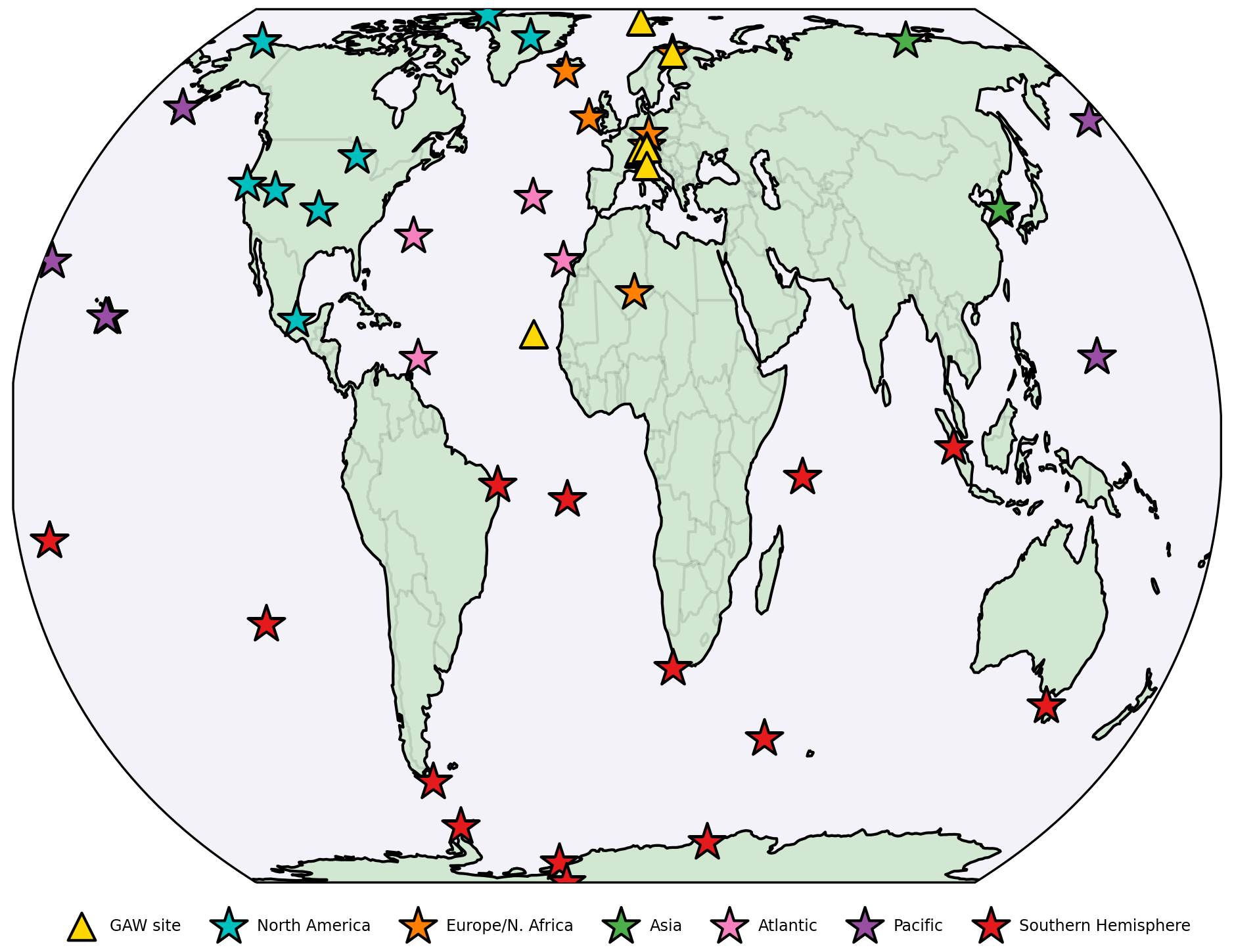
Figure 1Locations of GAW measurement sites and NOAA flask collection sites. The NOAA sites have been divided into six key regions for the evaluation, as shown by the colours of the symbols.
2.2.1 NOAA flask data sets
The National Oceanic and Atmospheric Administration (NOAA) and the Institute of Arctic and Alpine Research (INSTAAR) in Boulder, Colorado, operated a global VOC monitoring network established in 2004 based around flask sampling (Helmig et al., 2021). VOCs measurements were taken weekly or bi-weekly at 44 sites considered to be representative of the global background. The measurements were sampled in pairs from glass flasks. The NMVOC analysis is performed after the measurement of greenhouse gases and methane stable isotopic ratios.
The NMVOCs are measured by gas chromatography with flame ionisation detection and calibrated by a series of gravimetrically prepared synthetic and whole air standards. The programme operates under the umbrella of the World Meteorological Organization Global Atmospheric Watch (WMO GAW) and collaborates with international partners on the exchange of calibration standards and comparison of calibration scales. The INSTAAR laboratory was audited by the World Calibration Centre (WCC) for VOCs in 2008 and 2011. Five unknown standards were analysed, and results were reported to the WCC. Mean results of five repeated measurements of the provided standards deviated by < 1.5 % for ethane and < 0.8 % for propane from the certified values. These deviations are well within the criteria set by GAW. Uncertainties in the hydrocarbon data are estimated to be ≤ 5 % for mixing ratios of > 100 ppt (parts per trillion) and ≤ 5 ppt for mixing ratios < 100 ppt. For this study, 43 sites providing measurements over the relevant period were used in evaluating the model results.
Here, we use the measurements of ethane and propane and the sum of isobutane, n-butane, isopentane and n-pentane concentrations as “higher alkanes” to allow comparison with the GEOS-Chem ALK4 tracer. Data from 2016 and 2017 are used to evaluate the model performance.
2.2.2 WMO GAW data sets
The WMO GAW network has measurement sites in more than 80 countries, providing measurements of a range of compounds relevant to climate and air quality (WMO, 2021). However, NMVOC measurements are not made at all GAW sites. The available data sets relevant to this study represent a small subset of GAW sites and are entirely located in Europe or the North Atlantic (see Fig. 1). In this study, 2016 and 2017 measurements are used.
The model performance was evaluated by running its standard configuration using CEDS anthropogenic emissions for ethane, propane and the higher alkanes, plus geological emissions of ethane and propane. The simulated mass-weighted global mean tropospheric [OH] is 1.13 × 10⁶ molec. cm−3, which is within the estimated range from other chemistry models (Naik et al., 2013; Voulgarakis et al., 2013). The modelled tropospheric methane lifetime is 9.3 years, also within the expected range (Prather et al., 2012; Szopa et al., 2021). The root mean squared error between the model and the measurements is shown for each region. We also use a normalised mean bias metric to assess model performance.
3.1 Ethane
Figure 2 shows the comparison between measurements of ethane concentrations made as part of the NOAA flask network and those calculated by the model, divided into six regions. Orthogonal distance regression (Boggs and Donaldson, 1989) was used to calculate the line of best fit. The model underestimates ethane concentrations in all six regions shown in Fig. 1 with an overall bias of −35 %. The greatest NMB was found at measurements in the Atlantic (−49 %), with the lowest at Asian sites (−19 %). However, the largest absolute error was seen at Asian sites with a RMSE of 880 ppt, indicating poor model skill despite the smaller bias. At Asian, European and Atlantic sites, the underestimate appears more pronounced for higher concentrations, as indicated by the slope of the line of best fit. The error appears to be lower in the Southern Hemisphere, where measured concentrations tend to be lower; however, there remains a model bias of −32 %.
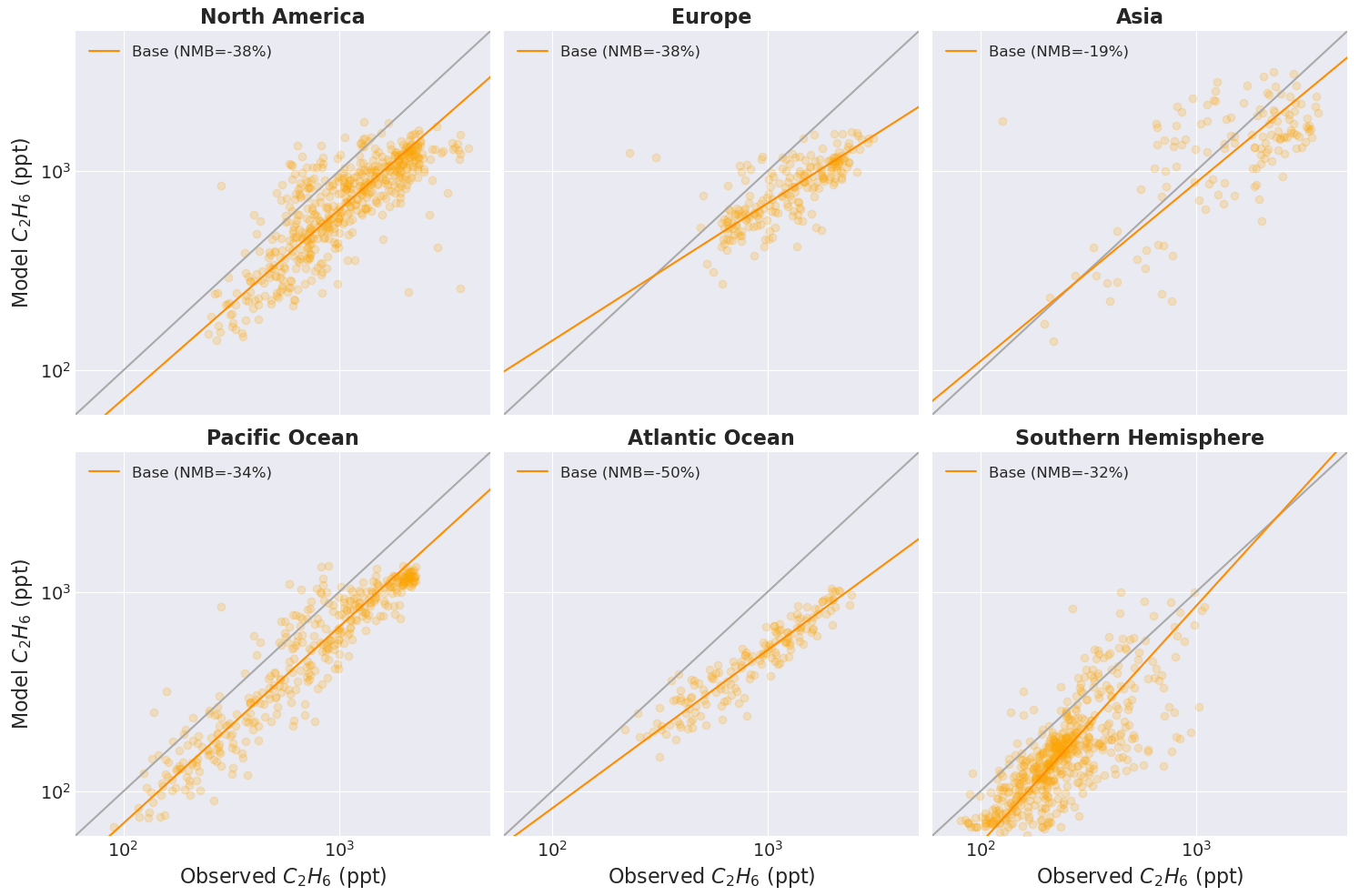
Figure 2Modelled and observed hourly mean ethane concentrations in ppt. Simulated concentrations are compared to observed values for 43 NOAA flask network sites for the years 2016–2017 (see Fig. 1). An orthogonal distance regression (orange line) and 1:1 regression (grey) are also included.
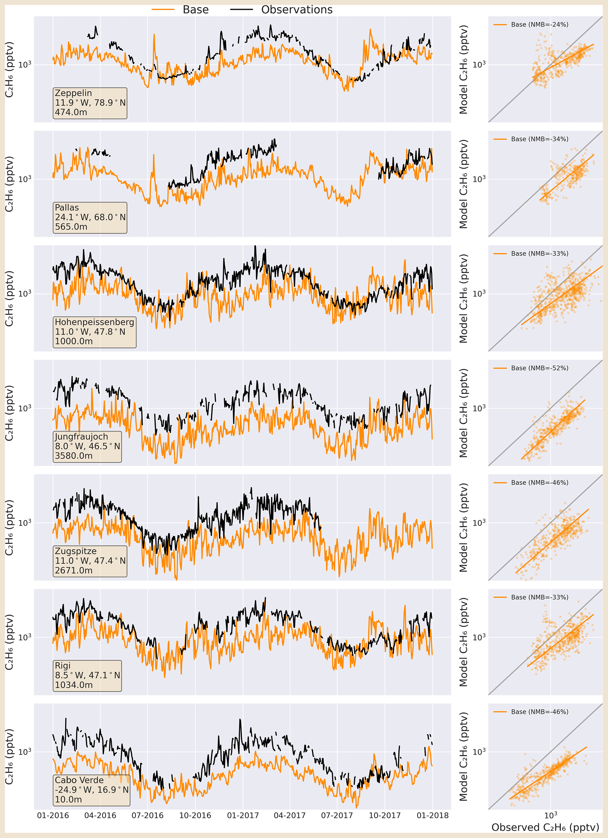
Figure 3Observed (black line) daily mean concentrations of ethane at seven GAW sites compared with simulated concentrations using default CEDS emissions (orange).
Figure 3 shows simulated and observed ethane at the seven GAW sites. Consistent with the flask data, the simulated ethane is underestimated in the model at all seven sites, with an overall low bias of −38 %. The RMSE ranges from 540 to 776 ppt across the sites, with greater error at sites situated above 1000 m altitude. In the summer months at Cabo Verde, Hohenpeissenberg and Zeppelin, there tends to be better agreement in absolute values between model and observations when concentrations are lower. However, winter and spring values are underestimated by as much as a factor of 2 at all sites. Overall the model simulation of ethane is consistent with previous modelling studies (Carmichael et al., 2003; Pozzer et al., 2007; Etiope and Ciccioli, 2009; Pozzer et al., 2010; Franco et al., 2016; Tzompa-Sosa et al., 2017; Dalsøren et al., 2018), with concentrations broadly underestimated by a factor of 2 across both flask measurements and GAW sites.
3.2 Propane
Figure 4 shows the comparison between the modelled simulation of propane and the measurements made at the NOAA flask sites. Like ethane, propane concentrations are substantially underestimated in the model, with a bias across all sites of −64 % and −59 % for the NOAA and GAW data sets, respectively. Measurements from Asia have the largest error, with a RMSE of 788 ppt and bias of −49 %, although there is significant scatter. Over the oceans and Southern Hemisphere, the RMSE ranges from 130 to 261 ppt, with the model often underestimating by more than a factor of 2 and with a bias up to 80 % in the Southern Hemisphere and Atlantic regions.
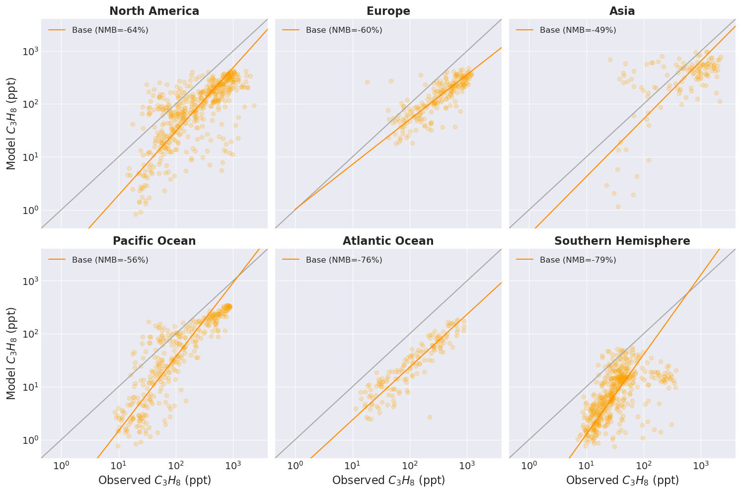
Figure 4Modelled and observed hourly mean propane concentrations in ppt. Simulated concentrations are compared to observed values for 43 NOAA flask network sites for the years 2016–2017 (see Fig. 1). An orthogonal distance regression (orange line) and 1:1 regression (grey) are also included.
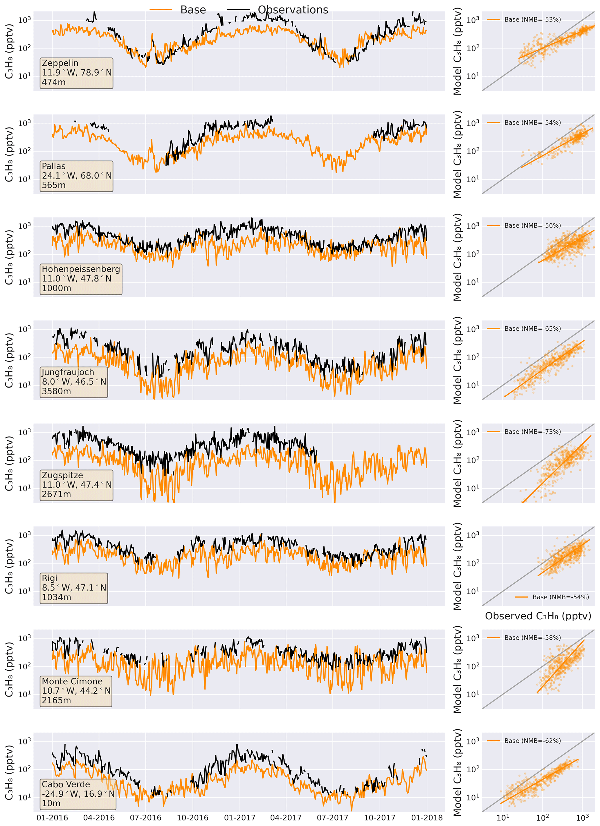
Figure 5Observed (black line) daily mean concentrations of propane at eight GAW sites compared with simulated concentrations using default CEDS emissions (orange).
The simulated propane concentrations compare similarly with the measurements at GAW sites across Europe and Cabo Verde (Fig. 5), with the model underestimating propane at every site by around a factor of 2. Similar to ethane, the largest absolute errors tend to be at the sites at higher latitudes, such as Zeppelin and Pallas, where the RMSE exceed 400 ppt; however, the NMB is similar at all sites, ranging from −53 % at Zeppelin to −73 % at Zugspitze.
The propane simulation is again consistent with previous work (Tzompa-Sosa et al., 2017; Dalsøren et al., 2018) and suggests an underestimate in the emissions of propane.
3.3 Higher alkanes
Model concentrations of the higher alkanes (ALK4 in GEOS-Chem) generally compare better to the observations than for ethane and propane (Fig. 6), with an overall overestimate of 11 %. The model generally underestimates higher alkanes at low concentrations, which may be in part due to the observations here including only butanes and pentanes, whereas the model aggregates a range of species including hexanes. Furthermore, it may be exacerbated by the limit of detection in measured values of ∼ 1 ppt (WMO, 2021), meaning that the model can reach concentrations that are much lower than can be reliably measured. This is particularly noticeable in the Pacific Ocean, where the observed values at concentrations above 100 ppt generally compare well with the model, but there are large underestimates at concentrations below 100 ppt, giving an overall RMSE of 187 ppt. Regionally, the model performs best over North America, with a NMB of 3 %, while there are larger overestimates at sites in Europe and Asia (biases of 46 % and 86 %, respectively). Concentrations at Atlantic or southern hemispheric sites tend to be underestimated, with a small overall overestimate in the Pacific (5 %) reflective of the model's tendency to underestimate higher alkanes where observed concentrations are low. Figure 7 shows the comparison between the simulated higher alkanes and those measured at eight GAW sites. Across all sites there is an overestimate in modelled concentrations of 68 %. Jungfraujoch, Zeppelin and Monte Cimone are the only sites with a negative bias, which is due to short peaks in measured concentrations which are not captured in the model, likely indicative of local pollution events. Whereas, in periods without such peaks, such as winter at Zeppelin and early 2017 at Monte Cimone, concentrations are more often overestimated. The remaining sites see a consistent overestimate in concentrations, with the model performing worst at Pallas (NMB = 193 %) and best at Rigi (72 %). The average model overestimate relative to the GAW sites is substantially greater than seen for the NOAA flask data set (11 %); however, it is similar in magnitude to the overestimate at European NOAA sites (46 %). This may be the result of local and regional emissions being important at the GAW sites which are all European apart from Cabo Verde, whereas many of the NOAA sites are very remote, marine or southern hemispheric where emissions are lower.
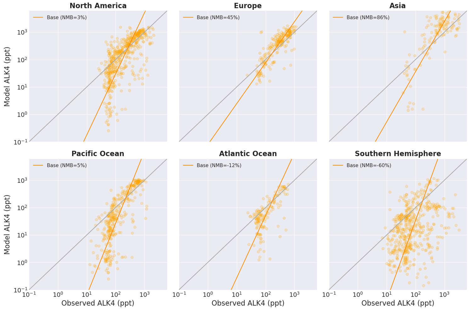
Figure 6Modelled and observed hourly mean ALK4 concentrations in ppt. Simulated concentrations are compared to observed values for 43 NOAA flask network sites for the years 2016–2017 and split into 6 regions as labelled. An orthogonal distance regression (orange line) and 1:1 regression (grey) are also included.
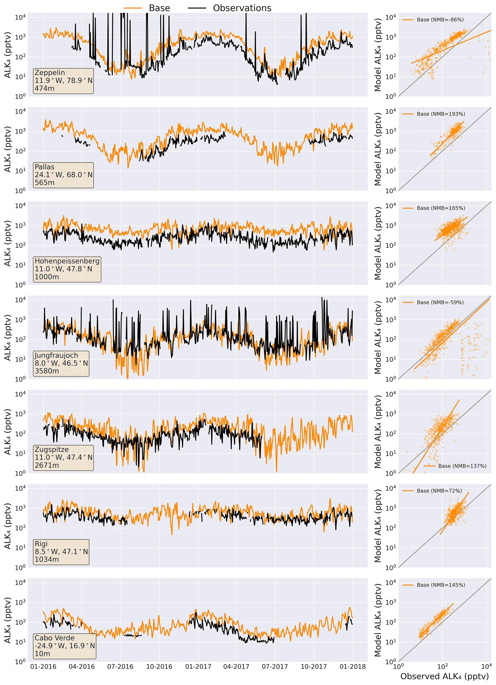
Figure 7Observed (black line) daily mean concentrations of higher alkanes at eight GAW sites compared with simulated concentrations using default CEDS emissions (orange).
3.3.1 Aromatic VOCs
As well as the alkanes, we also examine the model performance in simulating aromatic VOCs: benzene, toluene and xylene (Fig. 8). Measurements of these compounds are less widespread and were not available from the flask network. However, there are a number of GAW sites in Europe, as well as in Cabo Verde, with data available for the period relevant to this study. For benzene, the model generally performs fairly well, with a low bias of −12 % and the line of best fit showing no clear systematic bias. For toluene and xylene, there is very high variability in the comparison, resulting in larger underestimates in the model of −27 % and −55 % for toluene and xylene, respectively. The larger underestimate is likely a result of their very short atmospheric lifetimes coupled with uncertainty in emissions and model OH concentrations. Broadly, the model performs better overall for the aromatics than the alkanes, with relatively small underestimates across the available GAW sites rather than the factor of 2 difference seen for simulated ethane and propane concentrations. However, there is little correlation between the model and measurements for toluene or xylene.
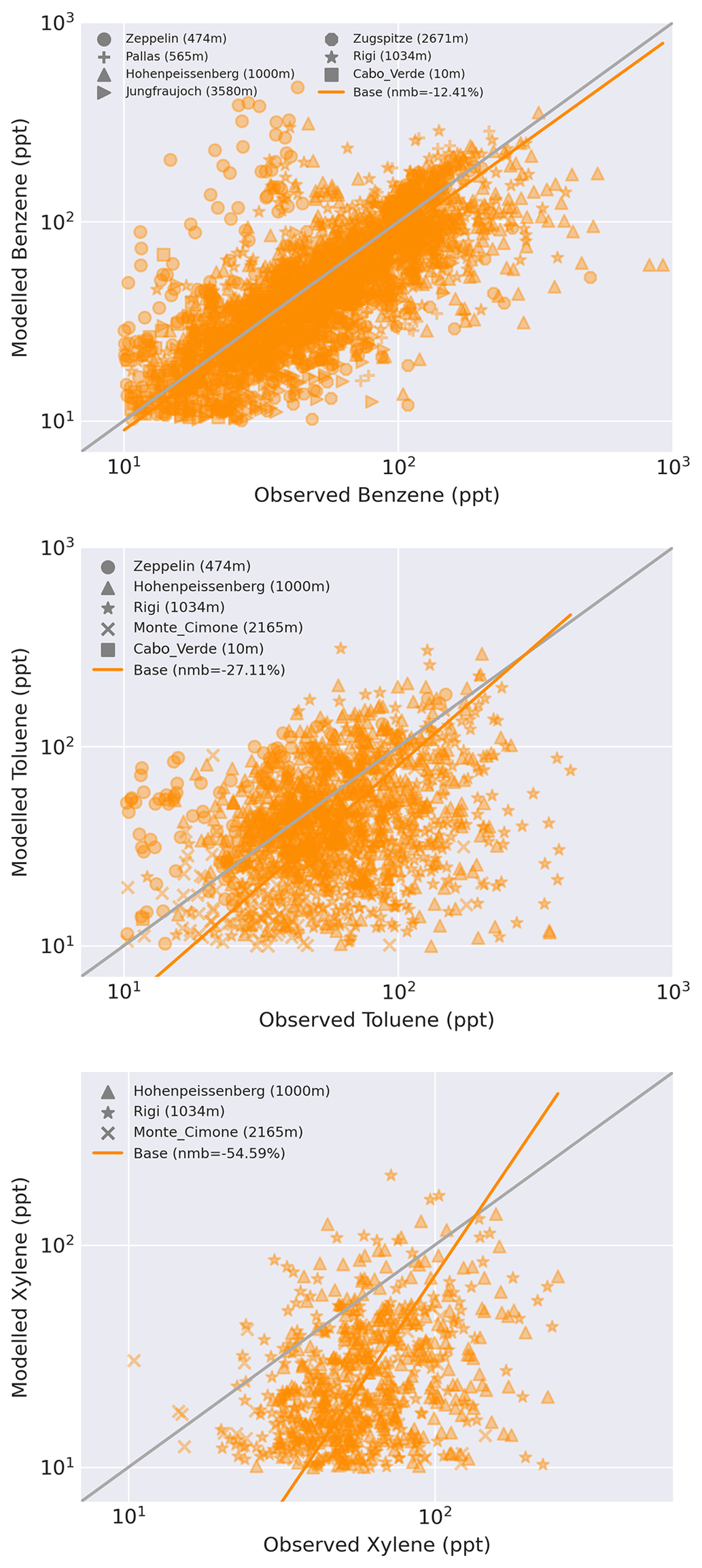
Figure 8Modelled and observed hourly mean mixing ratios of aromatic VOCs benzene, toluene and xylene in ppt. Simulated mixing ratios are compared to observed values from GAW sites in Europe and Cabo Verde with data available for 2016–2017. An orthogonal distance regression (orange line) and 1:1 regression (grey) are also included.
Propene measurements from Cabo Verde, Rigi and Hohenpeissenberg were also considered; however, the model performs very poorly, likely due to its short lifetime and a potential missing oceanic source which would be important in remote regions (Plass-Dülmer et al., 1993; Tripathi et al., 2020). Therefore, propene is not included further in this study.
3.3.2 Base model summary
The base simulation of ethane and propane appear consistent with previous work (Dalsøren et al., 2018; Emmons et al., 2015). The model underestimates concentrations by roughly a factor of 2, beyond what could reasonably be expected through a model overestimate of the global tropospheric OH concentration. Naik et al. (2013) estimate OH concentration at 1.1 × 10⁶ molec. cm−3 with an uncertainty of 7.0 %. Even if the model OH concentration were shifted to the lower end of this range, it would not be sufficient to extend the atmospheric lifetime enough to double the concentrations if the same emissions were maintained. Thus, given that there is no secondary chemical production of ethane or propane, we conclude that the current emissions of ethane and propane are underestimated.
The model simulation of higher alkanes (ALK4) overestimates the observations, which may be explained by the lumping of higher alkanes in GEOS-Chem. Although GEOS-Chem lumps butane, hexane and pentane into ALK4, the model then uses the OH rate constant associated with butane, which is slower than that for pentanes and hexanes (Atkinson et al., 2006), which would cause an overestimate. For aromatic VOCs, the observational network is less extensive but the model generally underestimates concentrations where measurements are available.
Given this, we now explore whether using the NMVOC speciations found in regional emissions estimates will improve the model performance.
Emission inventories with VOC-specific information are difficult to produce and therefore not available all over the world. In this study, we therefore focus on three major regions for which such data are available. Europe, the USA and China comprise three of the most important source regions for anthropogenic NMVOC emissions, contributing approximately 60 % of total global anthropogenic ethane emissions in the CEDS inventory.
The VOC speciation from a UK-based inventory is applied to all European VOC emissions. The UK National Atmospheric Emissions Inventory (NAEI) provides highly speciated and detailed emissions, allowing translation to model NMVOC species. The NAEI is the UK's official inventory submitted under the National Emissions Ceilings Regulations (NECR) and Gothenburg Protocol to the United Nations Economic Commission for Europe Convention on Long-Range Transboundary Air Pollution (Ingledew et al., 2023). The inventory covers over 400 individual sources of NMVOCs, with a large contribution from a diverse range of industrial and agricultural processes, combustion and use of solvents but with very few individually dominant sources. Further details on the methodology used to develop the NAEI and an explanation of emission trends are provided in the UK's annual Informative Inventory Report (Ingledew et al., 2023) and in AQEG (2020). Emissions of individual NMVOC species are estimated using source-specific speciation profiles which show the mass fraction of each species, or in some cases groups of species, emitted by the source (AQEG, 2020; Passant, 2002). Over 600 individual NMVOC species or species groups are covered in the speciation, based on sources in industry, regulators and in some cases literature sources and databases such as the U.S. Environmental Protection Agency's (EPA) SPECIATE database. The speciated inventory tends to be more uncertain than the inventory for total NMVOCs, and whereas the inventory for total NMVOCs is updated annually, the speciation profiles are only periodically updated when new information becomes available. Thus, trends in ethane and propane emissions for a sector shown by the NAEI are therefore a reflection of changes in total NMVOC emissions for the sector and do not normally reflect any changes over time in the speciation profile of the sector which may have occurred.
Speciated NMVOC emissions for the USA are from the U.S. EPA-distributed 2017 emissions modelling platform (2017 EMP). The 2017 EMP is derived from the 2017 National Emissions Inventories (US-EPA, 2021). The NEI is a synthesis of data gathered from state, local or tribal agencies and data directly produced at the EPA. Broadly, the NEI contains emissions data categorised by Source Classification Codes (SCCs). The SCC data are provided for compound classes of pollutants (e.g. NOx, VOC) at varying levels of spatial and temporal specificity. In the 2017 EMP, the NEI emissions from each SCC are spatially allocated to a model grid, temporally allocated to produce hour-specific rates and speciated for a specific photochemical model configuration. For more details about the 2017 EMP, refer to the 2017 technical support document (US-EPA, 2022). The 2017 EMP data used here were provided as monthly totals (from hourly) on a 12 km Lambert conformal grid; gases are speciated for the CMAQ (Community Multiscale Air Quality modelling system) Carbon Bond v6 revision 3 (CB6r3), and aerosols were speciated for CMAQ's aerosol module 7 (AE7). For use in GEOS-Chem, the 2017 EMP is translated for use with GEOS-Chem according to Henderson and Freese (2021) (https://doi.org/10.5281/zenodo.5122826). To summarise, the 2017 EMP is remapped to a longitude–latitude grid, vertical allocation is provided at high-level groupings of SCCs, speciation is translated via HEMCO configuration and hourly allocation is provided by HEMCO using the NEI99 inventory as a surrogate.
Speciated NMVOC emissions for China in 2017 are provided by the Multi-resolution Emission Inventory model for Climate and air pollution research (MEIC) (Li et al., 2017a; Zheng et al., 2018). The MEIC inventory is based on a series of models and nationwide survey data to estimate emissions of a range of gaseous and aerosol species in China (Li et al., 2017a). The MEIC provides several speciation mechanisms for NMVOC emissions, using composite source profiles to reduce uncertainty before mapping to specific chemical mechanisms following Carter (2010). Here we use the SAPRC07 methodology which lumps species based on functional groups (Carter, 2010), as this best matches the NMVOC species that are included in CEDS and GEOS-Chem. Further details on the methodology and associated uncertainties can be found in Li et al. (2014).
4.1 Re-speciating CEDS emissions using regional NMVOC emissions estimates
Figure 9 shows the NMVOC emissions speciation for Europe, USA and China for the three regional data sets compared to that from the CEDS global inventory. Ethane and propane emissions are considerably lower in the CEDS inventory for all three regions. The ratio of ethane emission to total NMVOC mass emissions is 0.02 over the USA in CEDS compared to 0.12 in the EPA/NEI emissions. This results in USA ethane emissions in the NEI being around 6 times larger than in CEDS. Propane is similarly higher in each regional inventory compared to CEDS (Fig. 9). This increase in ethane and propane is compensated for by lower ratios for the other VOC species, in particular the aromatics. Therefore, although the total NMVOC emissions in CEDS are almost identical to the totals in the regional inventories, they result in very different emissions of individual speciated VOCs. The substantially lower ethane and propane emissions in CEDS may explain the underestimate in simulated concentrations compared to observed values in Sect. 3.1 and 3.2.
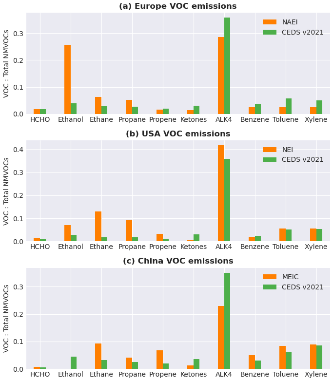
Figure 9VOC mass emissions as fractional mass of total NMVOC emissions for Europe (a), USA (b) and China (c). Regional emission estimates are in orange, and the CEDS VOC emissions from the same regions are in green.
We now apply the regional NMVOC speciations to the CEDS NMVOC emissions for each grid box of the relevant regions (USA, Europe and China). This re-speciation maintains the total mass of NMVOC emissions in each grid box but redistributes the total mass across individual VOC species according the regional speciation estimates. This is achieved through species-specific scale factors which are applied to the emissions at the point of input to the model. Regional estimates for 2017 are applied, as this was the most recent year with available emissions across every inventory used here. Emissions outside of these three regions are not changed, which notably includes India and the rest of Asia, Africa and all of the Southern Hemisphere. Following the adjustment of regional CEDS emissions as described above, the model was run again for the same period to assess the effect of the re-speciated emissions.
5.1 Ethane
In Fig. 10, simulated ethane using the re-speciated CEDS NMVOC emissions is compared with observations from the NOAA flask network together with the base model simulation. The model performance for ethane is substantially improved, increasing concentrations in all regions, particularly in the Northern Hemisphere where the re-speciation has been applied. The overall model bias has significantly reduced, from −35 % to −4 %, while the RMSE has roughly halved over North America, Europe and the Pacific and Atlantic ocean sites. The largest improvement is seen at sites in North America and Europe, where the bias has improved from −38 % and −38 % to −4 % and −4 %, respectively, effectively removing the model low bias. Similar improvements are found over the northern hemispheric marine sites, despite the emissions remaining the same in those regions. Asia is the only region in which the modelled ethane has not improved, going from an underestimate of 19 % to an overestimate of 26 %, while the RMSE increases from 880 to 933 ppt. This may indicate high uncertainty in VOC speciation in the regional database. Unsurprisingly, ethane concentrations in the Southern Hemisphere change the least in the new simulation, with RMSE decreasing from 147 to 139 ppt and NMB from −32 % to −23 %. As the re-speciation of anthropogenic emissions occurs entirely in the Northern Hemisphere, this is as expected, with the atmospheric lifetime of ethane (∼ 2 months; Helmig et al., 2014) being short enough to have only a small inter-hemispheric effect.
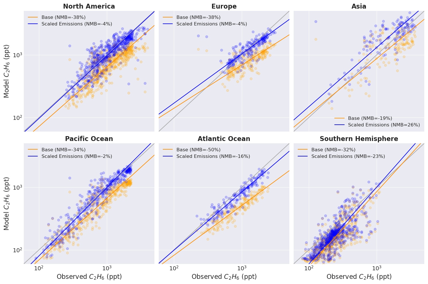
Figure 10Modelled and observed ethane concentrations in ppt. Simulated concentrations using CEDS emissions (orange) and regionally scaled CEDS emissions (blue) are compared to observed values at 43 NOAA flask network sites, divided into 6 regions, for the years 2016–2017.
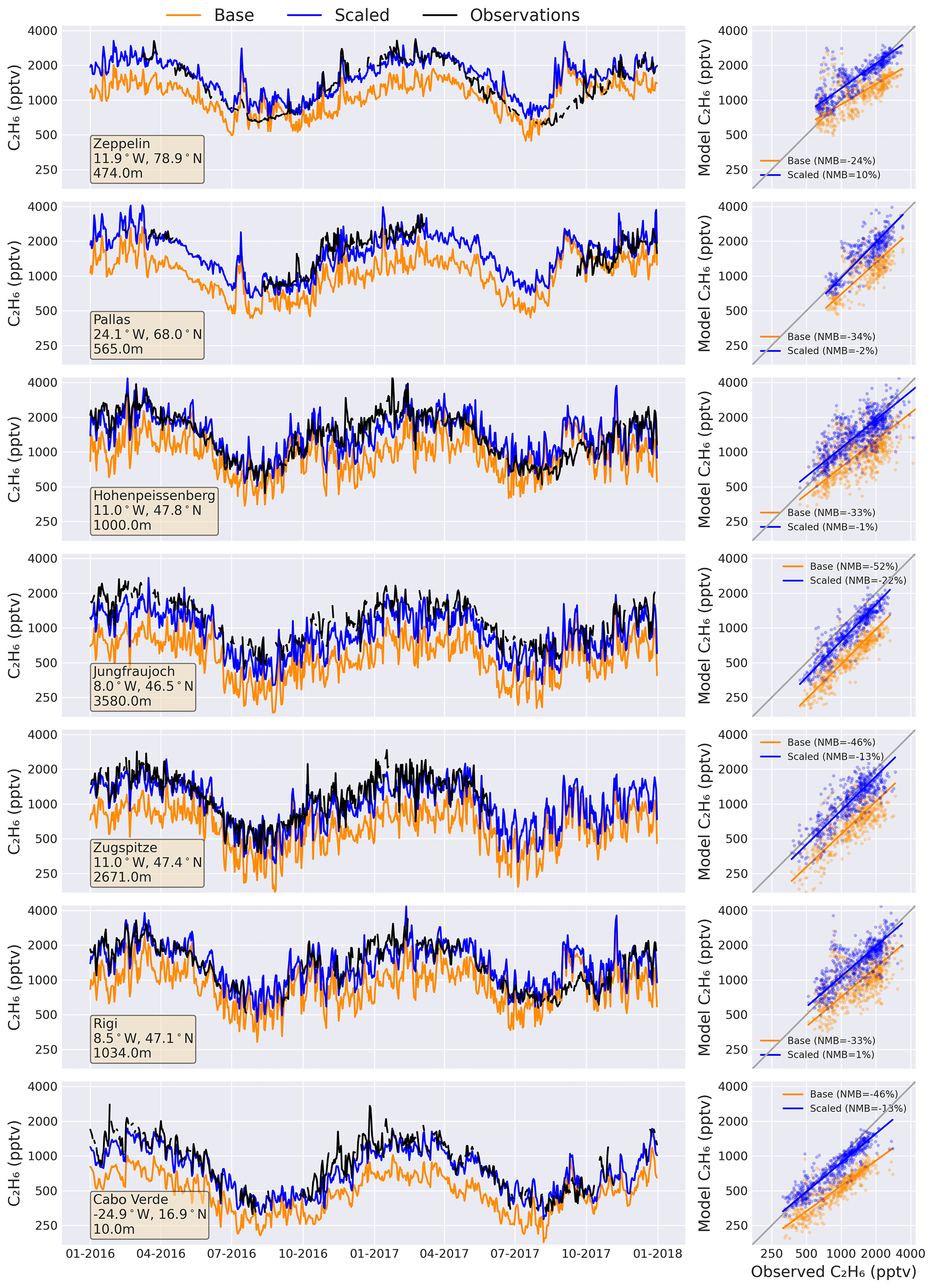
Figure 11Observed (black line) daily mean concentrations of ethane at seven GAW sites from 2016–2017, compared with the base GEOS-Chem simulation (orange) and the re-speciated CEDS emissions simulation (blue).
Figure 11 shows ethane concentrations from the re-speciated simulation against measurements from the GAW sites over the relevant period. As with the NOAA data, the model underestimate in ethane is decreased significantly from −38 % across the seven sites to −6 %. The improvement is consistent at all of the sites and throughout the measured period, approximately halving the RMSE at most sites and removing the systematic low bias. At the Zeppelin Observatory and Rigi, Germany, there are now slight model overestimates (10 % and 1 %, respectively), while the other sites remain slightly underestimated, with Jungfraujoch having the largest remaining bias (−22 %). Overall, the updated ethane simulations compare well with observed values throughout 2016–2017 at the GAW sites and in all global regions with NOAA flask data. This suggests that the model's underestimate of ethane concentrations in the base simulation may be the result of the CEDS mechanism of NMVOC speciation rather than errors in the total NMVOC emissions or the OH sink.
5.2 Propane
The re-speciation of the NMVOC emissions also results in improved model simulation of propane, with the bias compared to NOAA flask data improving from −64 % to −48 % (Fig. 12). As with ethane, propane concentrations increase at almost every site, as expected due to the increase in anthropogenic emissions of propane throughout the Northern Hemisphere. Over North America, the RMSE decreases by ∼ 20 % to 335 ppt, with the NMB improving from −64 % to −45 %. Similar improvements are seen across sites close to where the emissions have been changed in Asia and Europe, but unlike for ethane, there remains an underestimate in the model concentrations in all of the six regions. Sites in the Atlantic in particular maintain a large underestimate, with a NMB of −56 % in the updated simulation and a RMSE of 198 ppt. There is very little change in propane concentrations in the Southern Hemisphere due to the short atmospheric lifetime of propane (∼ 1 month; Rosado-Reyes and Francisco, 2007), which limits hemispherical mixing but is long enough to allow Northern Hemisphere concentrations remote from emissions sources to increase.
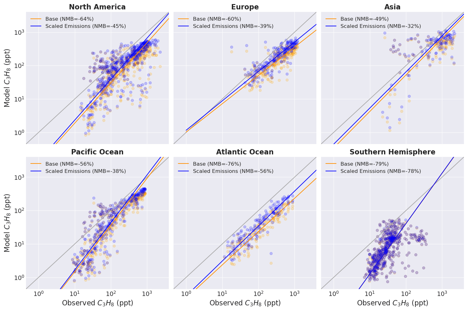
Figure 12Modelled and observed propane concentrations in ppt. Simulated concentrations using CEDS emissions (orange) and regionally scaled CEDS emissions (blue) are compared to observed values at 43 NOAA flask network sites, divided into 6 regions, for the years 2016–2017.
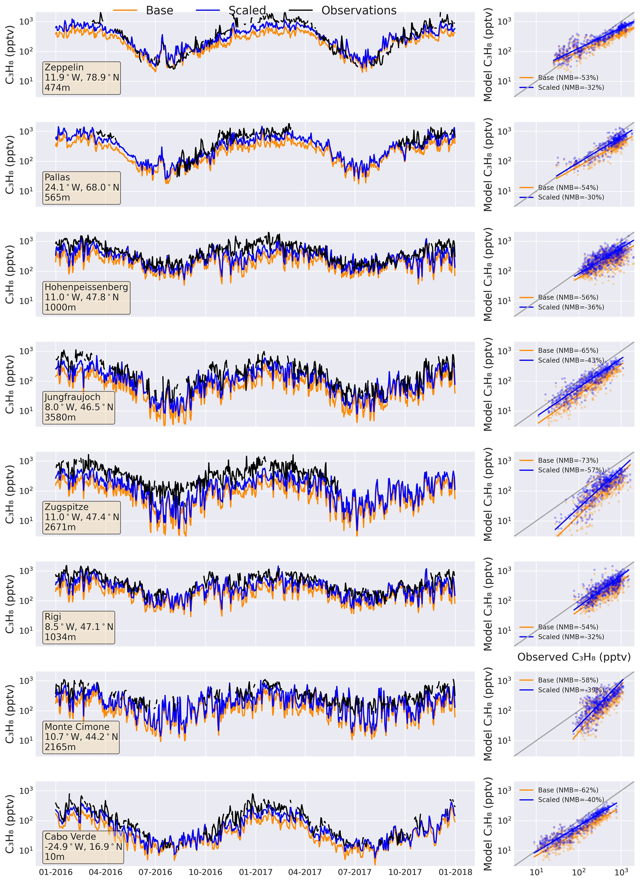
Figure 13Observed (black line) daily mean concentrations of propane at eight GAW sites from 2016–2017 compared with the base GEOS-Chem simulation (orange) and the re-speciated CEDS emissions simulation (blue).
Figure 13 shows the change in simulated propane concentrations relative to measurements from the eight GAW sites. The overall picture is similar to Fig. 12, with simulated propane concentrations increasing as a result of the re-speciation. This results in a decrease in the bias and error, although concentrations are still consistently underestimated by the model. The underestimate is smaller across all sites in the new simulation, with an overall NMB of −38 %, from −59 % in the base simulation. The highest-altitude sites of Jungfraujoch and Zugspitze–Schneefernerhaus have the largest underestimate in the re-speciated simulation, with NMBs of −43 % and −57 %, respectively. Unlike with ethane, there is no clear seasonality of the underestimate across the eight sites, and while the new simulation increases concentrations, the slope of the line of best fit is approximately consistent with that in the base simulation at almost all sites. These results show that increasing anthropogenic propane emissions through the re-speciation of NMVOCs improves the model's ability to replicate propane concentrations globally. However, the remaining low model bias across all observations suggests that the re-speciation does not fully address the problem. It is possible that emissions outside of the three regions for which emissions were re-speciated are important for propane and need to be included in the methodology to further improve modelled concentrations. In addition, there may be further propane sources currently missing from both global and regional emission inventories, resulting in an overall underestimate in propane and NMVOC emissions.
5.3 Higher alkanes
Changes to simulated higher-alkane concentrations are smaller than those for ethane and propane (Fig. 14), due to the smaller changes imposed during the re-speciation and the contrast in the direction of the change in different regions; anthropogenic emissions in North America increased, while decreasing in Europe and Asia (Fig. 8). Comparing to the NOAA flask data set (Fig. 14), the re-speciated simulation removes the small overestimate in the simulated higher-alkane concentration, with the overall NMB changing from 11 % to −1 %. The largest improvements are found at European and Asian sites, where decreased emissions through the re-speciation result in lower concentrations of higher alkanes. The NMB for European sites falls from 46 % to 24 %, while for Asia the change is 86 % to 55 %. Both regions therefore maintain a distinct overestimate in the model; however, model performance is substantially improved with the new speciation. In contrast, model performance in marine regions gets worse, with the NMB going from 5 % to −10 % and −12 % to −15 % for Pacific and Atlantic sites, respectively. Over North America, the model bias changes from a small overestimate to a small underestimate (3 % to −4 %), despite a 16 % increase in emissions of higher alkanes in the region. This is caused by larger decreases to emissions in other regions of the Northern Hemisphere (−20 % in Europe; −34 % in China), with the higher-alkane atmospheric lifetime of approximately 1 week (Hodnebrog et al., 2018) being sufficient to result in a small hemispheric impact. The change in the Southern Hemisphere, however, is negligible, as the lifetime is too short for inter-hemispheric mixing to occur. Figure 15 compares simulated higher-alkane concentrations with seven GAW sites across Europe and Cabo Verde. NMB is decreased at five of the seven sites, although changes in model performance tend to be small due to the relatively minor changes to total emissions. Simulated concentrations decrease at all sites, as expected, following the decrease in higher-alkane emissions from Europe and China. This results in a small increased in NMB at the Zeppelin Observatory in Norway and Jungfraujoch in Switzerland but otherwise brings the model into better agreement with background concentrations.
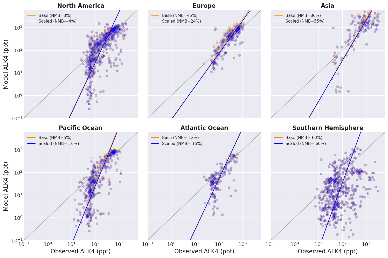
Figure 14Modelled and observed ALK4 concentrations in ppt. Simulated concentrations using CEDS emissions (orange) and regionally scaled CEDS emissions (blue) are compared to observed values at 43 NOAA flask network sites, divided into 6 regions, for the years 2016–2017.
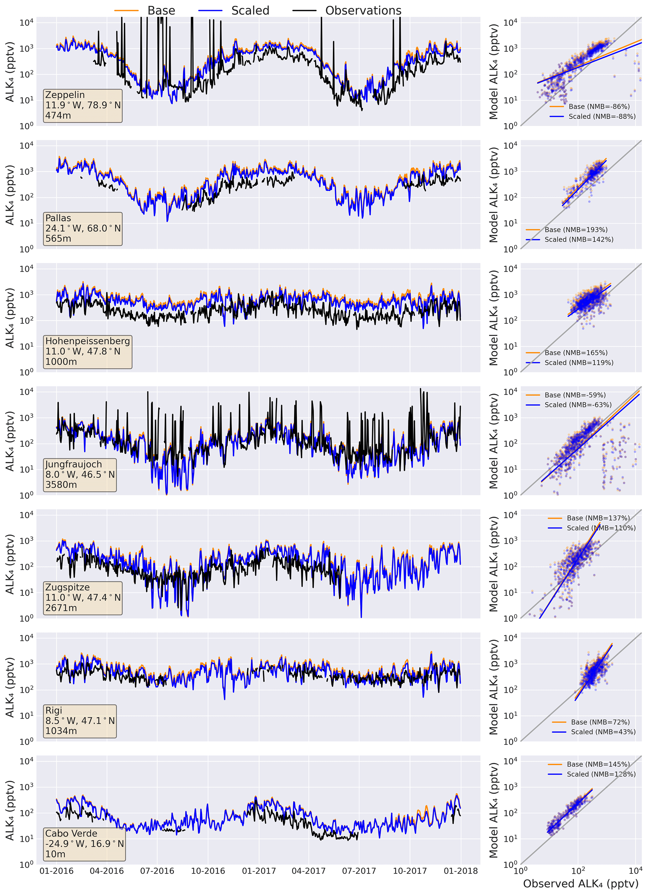
Figure 15Observed (black line) daily mean concentrations of ALK4 at seven GAW sites from 2016–2017, compared with the base GEOS-Chem simulation (orange) and the re-speciated CEDS emissions simulation (blue).
5.4 Aromatics
The re-speciation of anthropogenic VOCs has a largely detrimental effect on the simulation of aromatics. All three species included here were underestimated in the base model simulation relative to WMO GAW site data, and global emissions were decreased in the model during re-speciation, resulting in increased underestimation (Fig. 16). For benzene and toluene, this results in a doubling of the NMB, while for xylene the NMB also worsens from −55 % to −70 %. The re-speciation methodology therefore does not result in uniform improvement across all NMVOCs. There may be missing aromatic emission sources resulting in a consistent underestimate that cannot be rectified through improved NMVOC speciation.
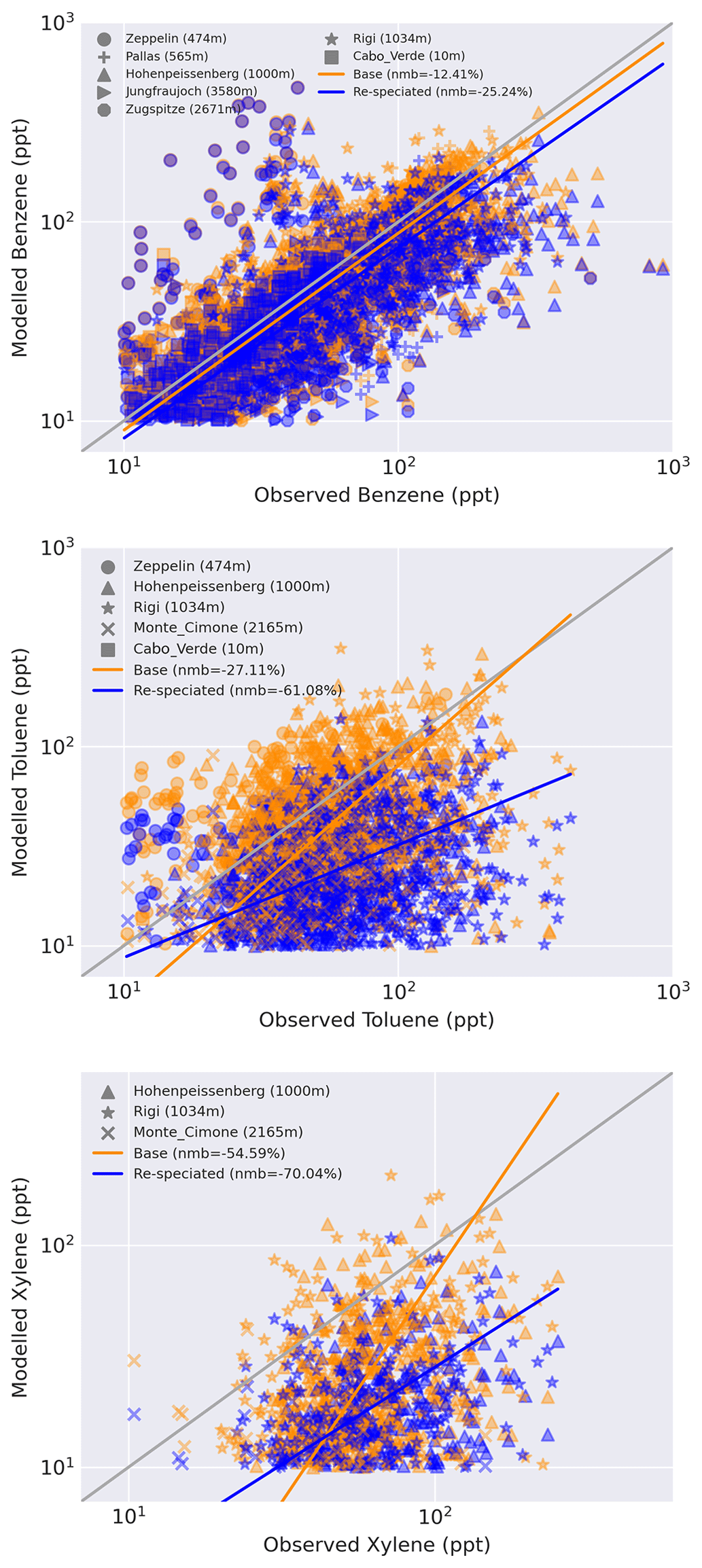
Figure 16Modelled and observed hourly mean mixing ratios of aromatics VOCs benzene, toluene and xylene in ppt. Simulated concentrations using CEDS emissions (orange) and re-speciated emissions (blue) are compared to observed values from GAW sites in Europe and Cabo Verde with data available for 2016–2017. An orthogonal distance regression and 1:1 regression (grey) are also included.
5.5 Discussion
In general, the re-speciation sees broad improvements in the model performance when simulating ethane. There are smaller improvements for propane and higher alkanes. The change to anthropogenic NMVOC emissions essentially removes the model underestimate in ethane, substantially deceasing the NMB and RMSE (Table 1). The bias in propane is decreased by 25 %–35 %, with a smaller relative decrease in RMSE, indicating that the speciation of NMVOC emissions is only part of the problem or that emissions from other regions (i.e. India and Southern Hemisphere) play an important role. Higher alkanes tend be overestimate drastically by the model in Europe (NMB = 81 %), as shown by the comparison with the GAW data sets (Fig. 15). This bias is larger than found by Ge et al. (2024) (approximately 50 %), likely due to differences in the sites included and the individual species aggregated. The comparison globally with flask data had a much smaller overestimate (Table 1). The overestimate of higher alkanes may be a result of an overestimate in emissions in the model or the result of lumping species in the model with the implied uncertainties in rate constants, creating an imperfect comparison with the measurements.
Table 1Mean RMSE and NMB values for each simulation and observational data set.
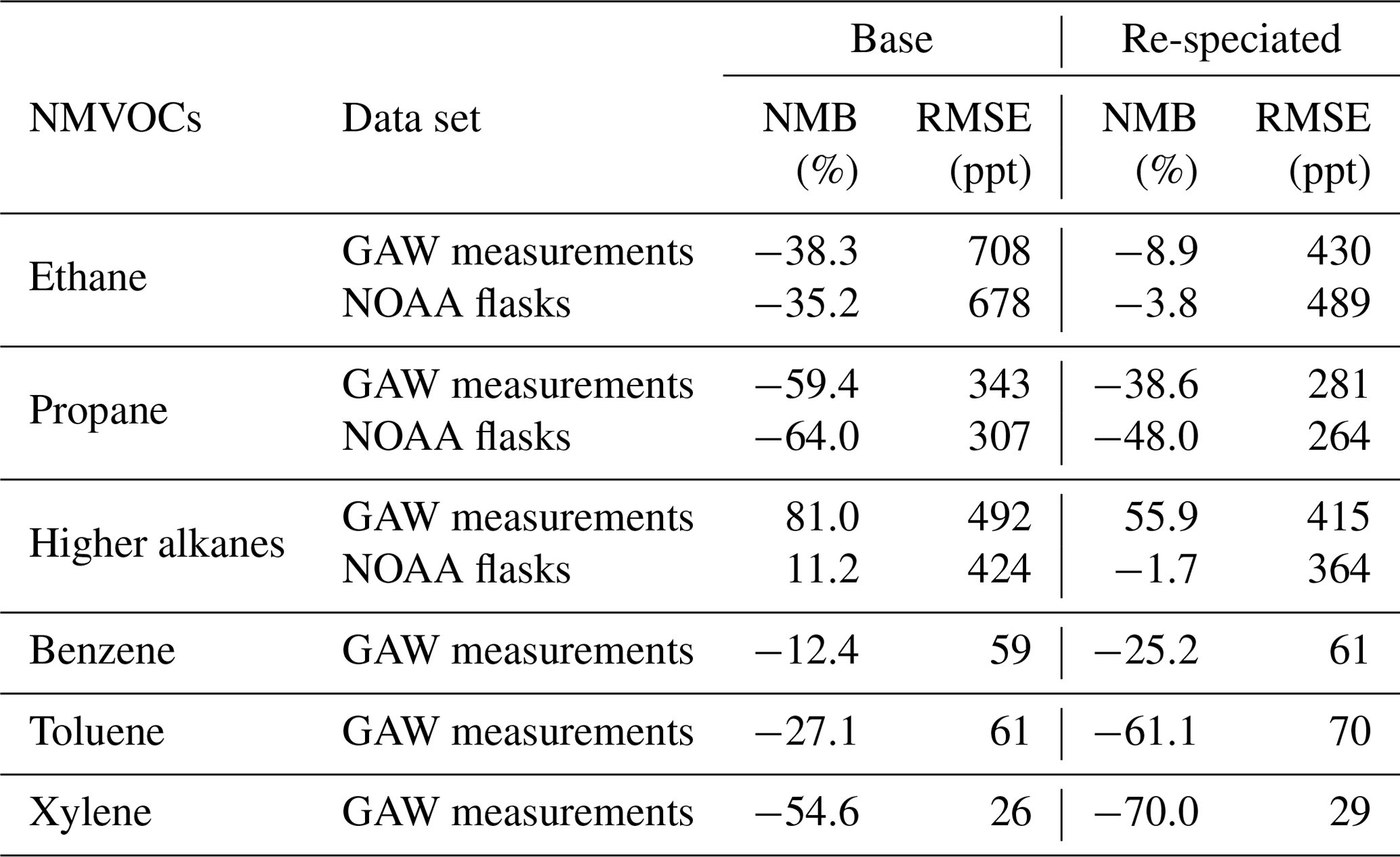
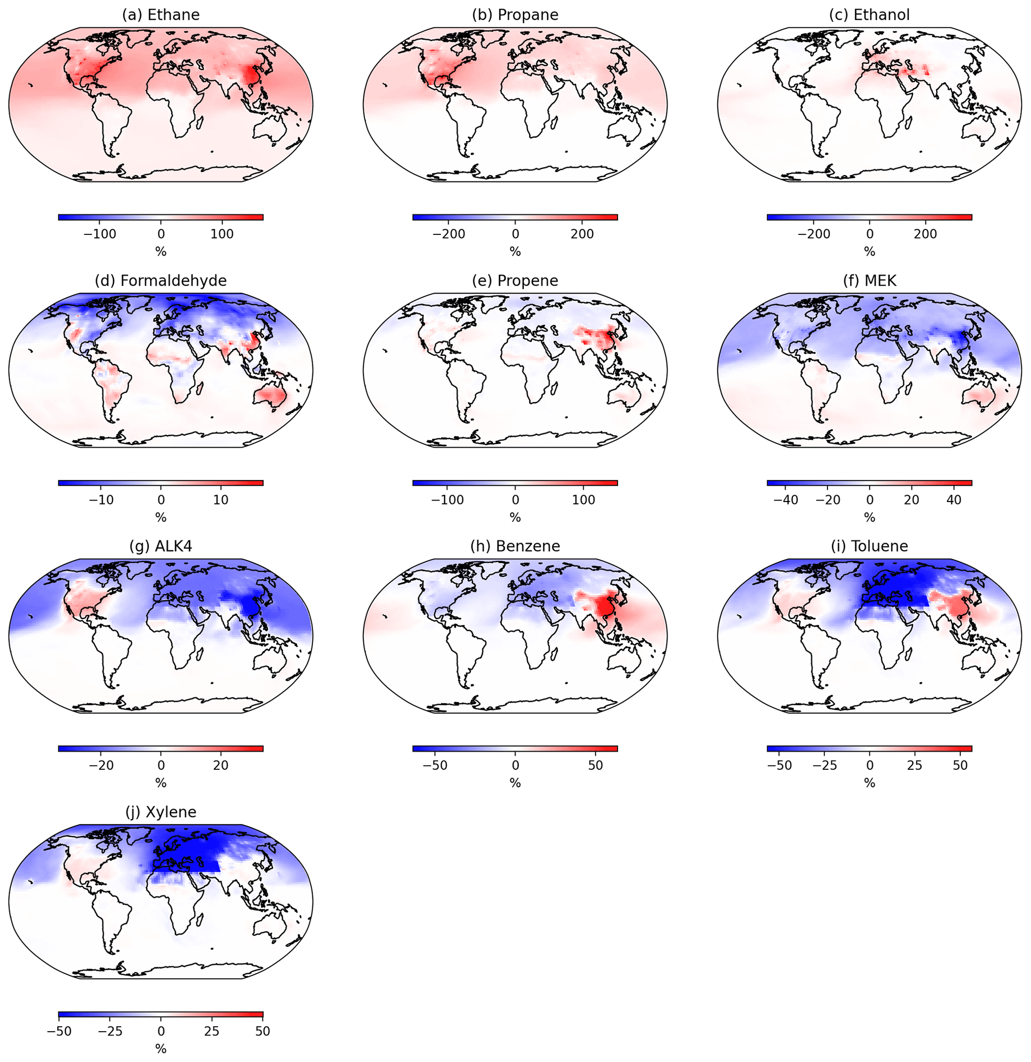
Figure 17Simulated percentage change in annual mean surface concentrations of various VOC species.
The percentage change in the global annual mean surface concentrations of the re-speciated VOCs is shown in Fig. 17. As expected, almost all of the changes in surface concentrations are restricted to the Northern Hemisphere, as the scale factors are only applied to emissions in this region. Increases in ethane and propane are largest in North America and China, where surface concentrations increased by more than 200 %, and the global tropospheric burdens of ethane and propane increased by 17 % and 34 %, respectively. Concentrations throughout the Northern Hemisphere are roughly doubled compared to the base simulation, due to the relatively long atmospheric lifetimes of ethane and propane. Other VOCs predominantly change in line with the scale factor applied in each region. Globally there is a decrease in the concentration of higher alkanes (ALK4) and aromatics (benzene, toluene and xylene), although with large regional variability. The scale of these changes is smaller than seen for ethane and propane, reflecting the smaller change to the emissions during re-speciation. Short-lived species such as ethanol, formaldehyde and propene have very localised impacts, while higher alkanes, ketones (MEK) and xylene lead to wider hemispheric impacts. Broadly, the changes imposed by the re-speciation of NMVOCs leads to large regional changes for each species. In the species for which we have observational data sets, the impact of the emissions changes range between a small improvement (ALK4) to a substantial increase in the model bias (toluene). However, given the limited observations coupled with remaining uncertainties in the emission sources for these compounds, the loss of model skill is minor in comparison to the improvement in ethane and propane.
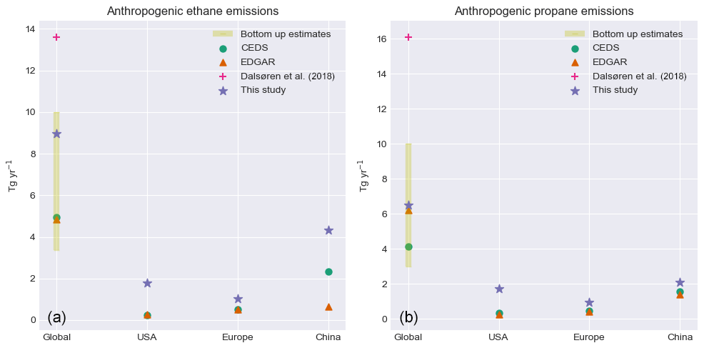
Figure 18Annual anthropogenic emissions of ethane (a) and propane (b) globally and in key source regions from global inventories (CEDS and EDGAR), a range of other bottom-up inventories (Dalsøren et al., 2018) and this study, following the re-speciation of CEDS emissions.
The changes in global and regional emissions of ethane and propane are shown in Fig. 18. The re-speciation process increased global ethane emissions from those in CEDS by 4 Tg yr−1, an increase of 81 %, with the largest absolute increase in emissions over China at 2 Tg yr−1. The re-speciation resulted in a smaller increase in global propane emissions of 2.3 Tg yr−1, which is a 57 % increase in the CEDS inventory. Globally, the re-speciation results in a substantial increase in anthropogenic emissions of both ethane and propane, but the total annual emissions remain comfortably within the range of the previous bottom-up studies (EDGAR v5.0, HTAPv2, RETRO, and POET; Dalsøren et al., 2018). The increases are, however, substantially lower than the optimised global total emissions estimated in Dalsøren et al. (2018). This may be a result of the global mean tropospheric OH concentration in those simulations being substantially higher than in GEOS-Chem (1.35 × 10⁶ vs. 1.13 × 10⁶ molec. cm−3), resulting in a faster loss rate of VOCs and meaning that larger emissions are required to simulate observed concentrations. A simple OH correction of the Dalsøren et al. (2018) study would suggest an emission of 11.4 Tg yr−1 for ethane which is closer to but slightly higher than the value of 9.0 Tg yr−1 used here (which does not included changes to emissions in India, Africa and the Southern Hemisphere). Given the differences in the OH concentrations, we likely have some agreement on the ethane source. A similar correction for propane would give an emissions of 13.4 Tg yr−1 – still substantially higher than those found here (6.5 Tg yr−1) – likely indicating that there is no agreement on the propane source.
5.6 Effect on atmospheric oxidation
In addition to directly influencing NMVOC concentrations, changes to NMVOC emissions can also influence atmospheric oxidation processes. Although the re-speciation of emissions maintains the total mass of NMVOCs emitted, individual NMVOC species have varying reactivity (Carter, 2010), and therefore, relative changes will affect oxidants such as O3 and OH. Figure 19 shows the simulated change in global mean surface concentrations of tropospheric O3 and OH, following the re-speciation of emissions. Globally, the changes are very small, with the surface annual mean change in O3 and OH of 3.8 % and −0.1 %, respectively. The minor change in global tropospheric OH maintains the mean annual concentration of 1.13 × 10⁶ molec. cm−3. The tropospheric ozone burden increases from 313.3 to 315.6 Tg yr−1, which is an increase of just 0.7 %. Regionally, there are larger impacts, with increases in both O3 and OH of ∼ 4 %–5 % in east China, with a decrease of a similar magnitude in OH over North America. However, despite large changes in relative concentrations of NMVOCs in the model, the changes to global atmospheric oxidation and tropospheric O3 in particular are small. On some levels, this is unsurprising. The methodology maintains the same mass of the emitted NMVOCs, meaning that only differences in the relative reactivity of VOC species would affect the chemistry. Furthermore, the vast majority of the atmosphere is in a NOx-limited regime for O3 production (Ivatt et al., 2022); thus, globally, changes in NMVOC concentrations are a relatively small lever on O3 concentrations. This is supported by Edwards and Evans (2017), who showed that non-isoprene NMVOCs contribute in a very minor way to global tropospheric O3 production, although can be important on regional scales.
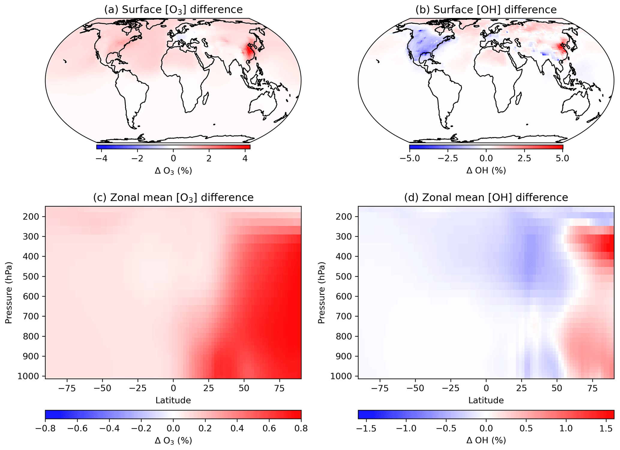
Figure 19Top panels show the simulated percentage change in annual mean surface concentrations of O3 (a) and OH (b). Lower panels (c, d) show the annual mean percentage change through the troposphere for the same species.
Overall, the impact on simulated oxidants concentrations is small. This indicates that the re-speciation of NMVOC emissions applied here can improve model performance for NMVOC concentrations without affecting the simulation of oxidants by the model. The changes seen are too small to impact the evaluation of model performance against observations.
Uncertainty in NMVOC speciation of anthropogenic emissions is large and at least partly responsible for poor model performance when simulating alkanes. We have shown that using regional NMVOC speciations rather than those used in CEDS significantly improves the simulation of ethane and propane concentrations in a global model. This effectively removes the underestimate in simulated ethane concentrations relative to observations. However, although modelled propane concentrations are improved, there remains a significant underestimate which might suggest a missing propane source. The simulation of the higher alkanes is limited by the model's use of an OH rate constant consistent with lumped higher alkanes. Despite this, the model performs well relative to observations of higher-alkane concentrations, both before and after re-speciation. Simulated concentrations of aromatic species of benzene, toluene and xylene generally degrade in the model following the re-speciation, resulting in an increase in the underestimate compared to measured concentrations. This deterioration is relatively small when compared to the improvement in the simulation of the alkanes and may be improved with further measurements of speciated NMVOCs.
The improvement in the simulation of alkanes was achieved without altering the total NMVOCs emitted in the model and without detrimental impacts on the majority of other VOC species. The secondary impact on atmospheric oxidation is small, due to the maintenance of total NMVOC emissions in the model and the model being largely in a NOx-limited regime, resulting in minor changes to global tropospheric O3 production.
The improvement in simulated propane and ethane shown here indicates that global emissions inventories should take into account detailed and up-to-date VOC regional speciation information. This would likely improve NMVOC simulations across various models, although differences in OH concentrations between models mean the impact of these changes will vary. In order to better understand the importance of model OH and the consistency of this conclusion, a multi-model analysis should be considered in the future.
GEOS-Chem version 14.0.1 used in this study (https://doi.org/10.5281/zenodo.7383492, The International GEOS-Chem User Community, 2022). Information and developments included in this version are available at http://wiki.seas.harvard.edu/geos-chem/index.php/GEOS-Chem_versions (last access: 21 May 2024). Model output, observational data sets and processing code are archived at https://doi.org/10.5281/zenodo.11259257 (Rowlinson, 2024). WMO GAW data sets are available from the EBAS Archive (https://ebas-data.nilu.no/; Carpenter et al., 2022). Data from the NOAA Global Monitoring Laboratory (GML) flask network are available at https://doi.org/10.15138/6AV8-GS57 (Helmig et al., 2021).
MJE, LJC and MJR developed the project. MJR performed the changes to emissions, ran the simulations and analysed the output. DH provided NOAA flask observations and guidance. TM, NP and BR provided the description of the NAEI inventory and guidance for its use. AL and LF provided the processed version of the NAEI inventory for use in GEOS-Chem. LJC, KAR and SP manage the Cape Verde Atmospheric Observatory (CVAO) site and data and provided the measurements used for evaluation. The paper was written by MJR with contributions from all co-authors.
At least one of the (co-)authors is a member of the editorial board of Atmospheric Chemistry and Physics. The peer-review process was guided by an independent editor, and the authors also have no other competing interests to declare.
Publisher's note: Copernicus Publications remains neutral with regard to jurisdictional claims made in the text, published maps, institutional affiliations, or any other geographical representation in this paper. While Copernicus Publications makes every effort to include appropriate place names, the final responsibility lies with the authors.
This project was undertaken on the Viking Computing Cluster, which is a high-performance computer facility provided by the University of York. We are grateful for computational support from the University of York high-performance computing service, Viking Computing Cluster and the research computing team. We thank WMO GAW and the individual sites that make up this network for the availability of the surface NMVOC data.
This research has been supported by the National Centre for Atmospheric Science (grant no. R8/H12/83/010).
This paper was edited by Kelley Barsanti and reviewed by two anonymous referees.
AQEG: Non-methane Volatile Organic Compounds in the UK, Report of the Air Quality Expert Group, Tech. rep., https://uk-air.defra.gov.uk/assets/documents/reports/cat09/2006240803_Non_Methane_Volatile_Organic_Compounds_in_the_UK.pdf (last access: 1 October 2023), 2020. a, b
Atkinson, R., Baulch, D. L., Cox, R. A., Crowley, J. N., Hampson, R. F., Hynes, R. G., Jenkin, M. E., Rossi, M. J., Troe, J., and IUPAC Subcommittee: Evaluated kinetic and photochemical data for atmospheric chemistry: Volume II – gas phase reactions of organic species, Atmos. Chem. Phys., 6, 3625–4055, https://doi.org/10.5194/acp-6-3625-2006, 2006. a, b
Aydin, M., Verhulst, K. R., Saltzman, E. S., Battle, M. O., Montzka, S. A., Blake, D. R., Qi Tang, Tang, Q., and Prather, M. J.: Recent decreases in fossil-fuel emissions of ethane and methane derived from firn air, Nature, 476, 198–201, https://doi.org/10.1038/nature10352, 2011. a
Bates, K. H., Jacob, D. J., Li, K., Ivatt, P. D., Evans, M. J., Yan, Y., and Lin, J.: Development and evaluation of a new compact mechanism for aromatic oxidation in atmospheric models, Atmos. Chem. Phys., 21, 18351–18374, https://doi.org/10.5194/acp-21-18351-2021, 2021. a
Bey, I., Jacob, D. J., Yantosca, R. M., Logan, J. A., Field, B. D., Fiore, A. M., Li, Q., Liu, H. Y., Mickley, L. J., and Schultz, M. G.: Global modeling of tropospheric chemistry with assimilated meteorology: Model description and evaluation, J. Geophys. Res.-Atmos., 106, 23073–23095, https://doi.org/10.1029/2001JD000807, 2001. a
Boggs, P. T. and Donaldson, J. R.: Orthogonal Distance Regression, Applied and Computational Mathematics Division, nistir 89-4197, https://nvlpubs.nist.gov/nistpubs/Legacy/IR/nistir89-4197.pdf (last access: 1 November 2022), 1989. a
Carmichael, G. R., Tang, Y., Kurata, G., Uno, I., Streets, D. G., Thongboonchoo, N., Woo, J.-H., Guttikunda, S., White, A., Wang, T., Blake, D. R., Atlas, E., Fried, A., Potter, B., Avery, M. A., Sachse, G. W., Sandholm, S. T., Kondo, Y., Talbot, R. W., Bandy, A., Thorton, D., and Clarke, A. D.: Evaluating regional emission estimates using the TRACE-P observations, J. Geophys. Res.-Atmos., 108, 8810, https://doi.org/10.1029/2002JD003116, 2003. a, b
Carpenter, L., Simpson, I., and Cooper, O.: Ground-Based Reactive Gas Observations Within the Global Atmosphere Watch (GAW) Network, 1–21, Springer, Germany, ISBN 978-981-15-2527-8, https://doi.org/10.1007/978-981-15-2527-8_8-1, 2022 (data available at: https://ebas-data.nilu.no/, last access: 6 February 2024). a, b
Carter, W. P.: Development of the SAPRC-07 chemical mechanism, Atmos. Environ., 44, 5324–5335, https://doi.org/10.1016/j.atmosenv.2010.01.026, 2010. a, b, c
Dalsøren, S. B., Myhre, G., Hodnebrog, O., Myhre, C. L., Stohl, A., Pisso, I., Schwietzke, S., Höglund-Isaksson, L., Helmig, D., Reimann, S., Sauvage, S., Schmidbauer, N., Read, K. A., Carpenter, L. J., Lewis, A. C., Punjabi, S., and Wallasch, M.: Discrepancy between simulated and observed ethane and propanelevels explained by underestimated fossil emissions, Nat. Geosci., 11, 178–184, https://doi.org/10.1038/s41561-018-0073-0, 2018. a, b, c, d, e, f, g, h, i, j, k, l, m, n
Dominutti, P., Nogueira, T., Fornaro, A., and Borbon, A.: One decade of VOCs measurements in São Paulo megacity: Composition, variability, and emission evaluation in a biofuel usage context, Sci. Total Environ., 738, 139790, https://doi.org/10.1016/j.scitotenv.2020.139790, 2020. a
Dominutti, P. A., Hopkins, J. R., Shaw, M., Mills, G. P., Le, H. A., Huy, D. H., Forster, G. L., Keita, S., Hien, T. T., and Oram, D. E.: Evaluating major anthropogenic VOC emission sources in densely populated Vietnamese cities, Environ. Pollut., 318, 120927, https://doi.org/10.1016/j.envpol.2022.120927, 2023. a
Edwards, P. M. and Evans, M. J.: A new diagnostic for tropospheric ozone production, Atmos. Chem. Phys., 17, 13669–13680, https://doi.org/10.5194/acp-17-13669-2017, 2017. a
EMEP/CEIP: Present state of emission data, EMEP/CEIP, https://www.ceip.at/webdab-emission-database/emissions-as-used-in-emep-models (last access: 6 July 2024), 2021. a
Emmons, L. K., Arnold, S. R., Monks, S. A., Huijnen, V., Tilmes, S., Law, K. S., Thomas, J. L., Raut, J.-C., Bouarar, I., Turquety, S., Long, Y., Duncan, B., Steenrod, S., Strode, S., Flemming, J., Mao, J., Langner, J., Thompson, A. M., Tarasick, D., Apel, E. C., Blake, D. R., Cohen, R. C., Dibb, J., Diskin, G. S., Fried, A., Hall, S. R., Huey, L. G., Weinheimer, A. J., Wisthaler, A., Mikoviny, T., Nowak, J., Peischl, J., Roberts, J. M., Ryerson, T., Warneke, C., and Helmig, D.: The POLARCAT Model Intercomparison Project (POLMIP): overview and evaluation with observations, Atmos. Chem. Phys., 15, 6721–6744, https://doi.org/10.5194/acp-15-6721-2015, 2015. a, b, c
Etiope, G. and Ciccioli, P.: Earth's Degassing: A Missing Ethane and Propane Source, Science, 323, 478–478, https://doi.org/10.1126/science.1165904, 2009. a, b, c, d, e
Etiope, G., Ciotoli, G., Schwietzke, S., and Schoell, M.: Gridded maps of geological methane emissions and their isotopic signature, Earth Syst. Sci. Data, 11, 1–22, https://doi.org/10.5194/essd-11-1-2019, 2019. a
Franco, B., Mahieu, E., Emmons, L. K., Tzompa-Sosa, Z. A., Fischer, E. V., Sudo, K., Bovy, B., Conway, S., Griffin, D., Hannigan, J. W., Strong, K., and Walker, K. A.: Evaluating ethane and methane emissions associated with the development of oil and natural gas extraction in North America, Environ. Res. Lett., 11, 044010, https://doi.org/10.1088/1748-9326/11/4/044010, 2016. a, b, c
Fry, M. M., Naik, V., West, J. J., Schwarzkopf, M. D., Fiore, A. M., Collins, W. J., Dentener, F. J., Shindell, D. T., Atherton, C., Bergmann, D., Duncan, B. N., Hess, P., MacKenzie, I. A., Marmer, E., Schultz, M. G., Szopa, S., Wild, O., and Zeng, G.: The influence of ozone precursor emissions from four world regions on tropospheric composition and radiative climate forcing, J. Geophys. Res.-Atmos., 117, D07306, https://doi.org/10.1029/2011JD017134, 2012. a
Ge, Y., Solberg, S., Heal, M., Reimann, S., van Caspel, W., Hellack, B., Salameh, T., and Simpson, D.: Evaluation of modelled versus observed NMVOC compounds at EMEP sites in Europe, EGUsphere [preprint], https://doi.org/10.5194/egusphere-2023-3102, 2024. a, b
Gelaro, R., McCarty, W., Suarez, M. J., Todling, R., Molod, A., Takacs, L., Randles, C. A., Darmenov, A., Bosilovich, M. G., Reichle, R., Wargan, K., Coy, L., Cullather, R., Draper, C., Akella, S., Buchard, V., Conaty, A., da Silva, A. M., Gu, W., Kim, G.-K., Koster, R., Lucchesi, R., Merkova, D., Nielsen, J. E., Partyka, G., Pawson, S., Putman, W., Rienecker, M., Schubert, S. D., Sienkiewicz, M., and Zhao, B.: The Modern-Era Retrospective Analysis for Research and Applications, Version 2 (MERRA-2), J. Climate, 30, 5419–5454, https://doi.org/10.1175/JCLI-D-16-0758.1, 2017. a
Guenther, A., Hewitt, C. N., Erickson, D., Fall, R., Geron, C., Graedel, T., Harley, P., Klinger, L., Lerdau, M., Mckay, W. A., Pierce, T., Scholes, B., Steinbrecher, R., Tallamraju, R., Taylor, J., and Zimmerman, P.: A global model of natural volatile organic compound emissions, J. Geophys. Res.-Atmos., 100, 8873–8892, https://doi.org/10.1029/94JD02950, 1995. a, b
Helmig, D., Petrenko, V., Martinerie, P., Witrant, E., Röckmann, T., Zuiderweg, A., Holzinger, R., Hueber, J., Thompson, C., White, J. W. C., Sturges, W., Baker, A., Blunier, T., Etheridge, D., Rubino, M., and Tans, P.: Reconstruction of Northern Hemisphere 1950–2010 atmospheric non-methane hydrocarbons, Atmos. Chem. Phys., 14, 1463–1483, https://doi.org/10.5194/acp-14-1463-2014, 2014. a, b
Helmig, D., Rossabi, S., Hueber, J., Tans, P., Montzka, S. A., Masarie, K., Thoning, K., Plass-Duelmer, C., Claude, A., Carpenter, L. J., Lewis, A. C., Punjabi, S., Reimann, S., Vollmer, M. K., Steinbrecher, R., Hannigan, J. W., Emmons, L. K., Mahieu, E., Franco, B., Smale, D., and Pozzer, A.: Reversal of global atmospheric ethane and propane trends largely due to US oil and natural gas production, Nat. Geosci., 9, 490–495, https://doi.org/10.1038/ngeo2721, 2016. a
Helmig, D., Hueber, J., Tans, P., University Of Colorado Institute Of Arctic And Alpine Research (INSTAAR), and NOAA GML CCGG Group: Flask-Air Sample Measurements of Atmospheric Non Methane Hydrocarbons Mole Fractions from the NOAA GML Carbon Cycle Surface Network at Global and Regional Background Sites, 2004–2016 (Version 2021.05.04), University of Colorado Institute of Arctic and Alpine Research (INSTAAR), NOAA Global Monitoring Laboratory [data set], https://doi.org/10.15138/6AV8-GS57, 2021. a, b, c, d
Henderson, B. and Freese, L.: Preparation of GEOS-Chem Emissions from CMAQ, Zenodo [code], https://doi.org/10.5281/zenodo.5122826, 2021. a
Hodnebrog, O., Dalsøren, S. B., and Myhre, G.: Lifetimes, direct and indirect radiative forcing, and global warming potentials of ethane (C2H6), propane (C3H8), and butane (C4H10), Atmos. Sci. Lett., 19, e804, https://doi.org/10.1002/asl.804, 2018. a
Hodzic, A., Kasibhatla, P. S., Jo, D. S., Cappa, C. D., Jimenez, J. L., Madronich, S., and Park, R. J.: Rethinking the global secondary organic aerosol (SOA) budget: stronger production, faster removal, shorter lifetime, Atmos. Chem. Phys., 16, 7917–7941, https://doi.org/10.5194/acp-16-7917-2016, 2016. a
Hoesly, R. M., Smith, S. J., Feng, L., Klimont, Z., Janssens-Maenhout, G., Pitkanen, T., Seibert, J. J., Vu, L., Andres, R. J., Bolt, R. M., Bond, T. C., Dawidowski, L., Kholod, N., Kurokawa, J.-I., Li, M., Liu, L., Lu, Z., Moura, M. C. P., O'Rourke, P. R., and Zhang, Q.: Historical (1750–2014) anthropogenic emissions of reactive gases and aerosols from the Community Emissions Data System (CEDS), Geosci. Model Dev., 11, 369–408, https://doi.org/10.5194/gmd-11-369-2018, 2018. a, b, c
Ingledew, D., Churchill, S., Richmond, B., MacCarthy, J., Avis, K., Brown, P., Del Vento, S., Galatioto, F., Gorji, S., Karagianni, E., Kelsall, A., Misra, A., Murrells, T., Passant, N., Pearson, B., Richardson, J., Stewart, R., Thistlethwaite, G., Tsagatakis, I., Wakeling, D., Walker, C., Wiltshire, J., Wong, J., and Yardley, R.: UK Informative Inventory Report (1990 to 2021), Tech. rep., NAEI, https://uk-air.defra.gov.uk/assets/documents/reports/cat09/2303151609_UK_IIR_2023_Submission.pdf (last access: 22 October 2023), 2023. a, b
Ivatt, P. D., Evans, M. J., and Lewis, A. C.: Suppression of surface ozone by an aerosol-inhibited photochemical ozone regime, Nat. Geosci., 15, 536–540, https://doi.org/10.1038/s41561-022-00972-9, 2022. a
Kirschke, S., Bousquet, P., Ciais, P., Saunois, M., Canadell, J. G., Dlugokencky, E. J., Bergamaschi, P., Bergmann, D., Blake, D. R., Bruhwiler, L., Cameron-Smith, P., Castaldi, S., Chevallier, F., Feng, L., Fraser, A., Heimann, M., Hodson, E. L., Houweling, S., Josse, B., Fraser, P. J., Krummel, P. B., Lamarque, J.-F., Langenfelds, R. L., Le Quéré, C., Naik, V., O'Doherty, S., Palmer, P. I., Pison, I., Plummer, D., Poulter, B., Prinn, R. G., Rigby, M., Ringeval, B., Santini, M., Schmidt, M., Shindell, D. T., Simpson, I. J., Spahni, R., Steele, L. P., Strode, S. A., Sudo, K., Szopa, S., van der Werf, G. R., Voulgarakis, A., van Weele, M., Weiss, R. F., Williams, J. E., and Zeng, G.: Three decades of global methane sources and sinks, Nat. Geosci., 6, 813–823, https://doi.org/10.1038/ngeo1955, 2013. a
Koffi, B., Dentener, F., Janssens-Maenhout, G., Guizzardi, D., Crippa, M., Diehl, T., Galmarini, S., and Solazzo, E.: Hemispheric Transport of Air Pollution (HTAP): Specification of the HTAP2 experiments: Ensuring harmonized modelling, Tech. rep., Hemispheric Transport Air Pollution (HTAP), Publications Office of the European Union, Luxembourg, https://doi.org/10.2788/725244, 2016. a
Li, M., Zhang, Q., Streets, D. G., He, K. B., Cheng, Y. F., Emmons, L. K., Huo, H., Kang, S. C., Lu, Z., Shao, M., Su, H., Yu, X., and Zhang, Y.: Mapping Asian anthropogenic emissions of non-methane volatile organic compounds to multiple chemical mechanisms, Atmos. Chem. Phys., 14, 5617–5638, https://doi.org/10.5194/acp-14-5617-2014, 2014. a
Li, M., Liu, H., Geng, G., Hong, C., Liu, F., Song, Y., Tong, D., Zheng, B., Cui, H., Man, H., Zhang, Q., and He, K.: Anthropogenic emission inventories in China: a review, Nat. Sci. Rev., 4, 834–866, https://doi.org/10.1093/nsr/nwx150, 2017a. a, b, c
Li, M., Zhang, Q., Kurokawa, J.-I., Woo, J.-H., He, K., Lu, Z., Ohara, T., Song, Y., Streets, D. G., Carmichael, G. R., Cheng, Y., Hong, C., Huo, H., Jiang, X., Kang, S., Liu, F., Su, H., and Zheng, B.: MIX: a mosaic Asian anthropogenic emission inventory under the international collaboration framework of the MICS-Asia and HTAP, Atmos. Chem. Phys., 17, 935–963, https://doi.org/10.5194/acp-17-935-2017, 2017b. a
McDuffie, E. E., Smith, S. J., O'Rourke, P., Tibrewal, K., Venkataraman, C., Marais, E. A., Zheng, B., Crippa, M., Brauer, M., and Martin, R. V.: A global anthropogenic emission inventory of atmospheric pollutants from sector- and fuel-specific sources (1970–2017): an application of the Community Emissions Data System (CEDS), Earth Syst. Sci. Data, 12, 3413–3442, https://doi.org/10.5194/essd-12-3413-2020, 2020. a, b
Monks, P. S., Archibald, A. T., Colette, A., Cooper, O., Coyle, M., Derwent, R., Fowler, D., Granier, C., Law, K. S., Mills, G. E., Stevenson, D. S., Tarasova, O., Thouret, V., von Schneidemesser, E., Sommariva, R., Wild, O., and Williams, M. L.: Tropospheric ozone and its precursors from the urban to the global scale from air quality to short-lived climate forcer, Atmos. Chem. Phys., 15, 8889–8973, https://doi.org/10.5194/acp-15-8889-2015, 2015. a
Naik, V., Voulgarakis, A., Fiore, A. M., Horowitz, L. W., Lamarque, J.-F., Lin, M., Prather, M. J., Young, P. J., Bergmann, D., Cameron-Smith, P. J., Cionni, I., Collins, W. J., Dalsøren, S. B., Doherty, R., Eyring, V., Faluvegi, G., Folberth, G. A., Josse, B., Lee, Y. H., MacKenzie, I. A., Nagashima, T., van Noije, T. P. C., Plummer, D. A., Righi, M., Rumbold, S. T., Skeie, R., Shindell, D. T., Stevenson, D. S., Strode, S., Sudo, K., Szopa, S., and Zeng, G.: Preindustrial to present-day changes in tropospheric hydroxyl radical and methane lifetime from the Atmospheric Chemistry and Climate Model Intercomparison Project (ACCMIP), Atmos. Chem. Phys., 13, 5277–5298, https://doi.org/10.5194/acp-13-5277-2013, 2013. a, b
Nicewonger, M. R., Verhulst, K. R., Aydin, M., and Saltzman, E. S.: Preindustrial atmospheric ethane levels inferred from polar ice cores: A constraint on the geologic sources of atmospheric ethane and methane, Geophys. Res. Lett., 43, 214–221, https://doi.org/10.1002/2015GL066854, 2016. a, b
Passant, N. R.: Speciation of UK emissions of non-methane volatile organic compounds, NAEI Report AEAT/ENV/R/0545 prepared for DETR Air and Environmental Quality Division, Tech. rep., https://uk-air.defra.gov.uk/assets/documents/reports/empire/AEAT_ENV_0545_final_v2.pdf (last access: 22 October 2023), 2002. a
Plass-Dülmer, C., Khedim, A., Koppmann, R., Johnen, F. J., Rudolph, J., and Kuosa, H.: Emissions of light nonmethane hydrocarbons from the Atlantic into the atmosphere, Global Biogeochem. Cy., 7, 211–228, https://doi.org/10.1029/92GB02361, 1993. a
Pozzer, A., Jöckel, P., Tost, H., Sander, R., Ganzeveld, L., Kerkweg, A., and Lelieveld, J.: Simulating organic species with the global atmospheric chemistry general circulation model ECHAM5/MESSy1: a comparison of model results with observations, Atmos. Chem. Phys., 7, 2527–2550, https://doi.org/10.5194/acp-7-2527-2007, 2007. a, b, c
Pozzer, A., Pollmann, J., Taraborrelli, D., Jöckel, P., Helmig, D., Tans, P., Hueber, J., and Lelieveld, J.: Observed and simulated global distribution and budget of atmospheric C2–C5 alkanes, Atmos. Chem. Phys., 10, 4403–4422, https://doi.org/10.5194/acp-10-4403-2010, 2010. a, b
Prather, M. J., Holmes, C. D., and Hsu, J.: Reactive greenhouse gas scenarios: Systematic exploration of uncertainties and the role of atmospheric chemistry, Geophys. Res. Lett., 39, L09803, https://doi.org/10.1029/2012GL051440, 2012. a
Rosado-Reyes, C. M. and Francisco, J. S.: Atmospheric oxidation pathways of propane and its by-products: Acetone, acetaldehyde, and propionaldehyde, J. Geophys. Res.-Atmos., 112, D14310, https://doi.org/10.1029/2006JD007566, 2007. a
Rowlinson, M.: Revising VOC emissions speciation improves the simulation of global background of ethane and propane, Zenodo [data set and code], https://doi.org/10.5281/zenodo.11259257, 2024. a
Simpson, D., Winiwarter, W., Börjesson, G., Cinderby, S., Ferreiro, A., Guenther, A., Hewitt, C. N., Janson, R., Khalil, M. A. K., Owen, S., Pierce, T. E., Puxbaum, H., Shearer, M., Skiba, U., Steinbrecher, R., Tarrasón, L., and Öquist, M. G.: Inventorying emissions from nature in Europe, J. Geophys. Res.-Atmos., 104, 8113–8152, https://doi.org/10.1029/98JD02747, 1999. a
Simpson, I. J., Andersen, M. P. S., Meinardi, S., Bruhwiler, L., Blake, N. J., Helmig, D., Rowland, F. S., and Blake, D. R.: Long-term decline of global atmospheric ethane concentrations and implications for methane, Nature, 488, 490–494, https://doi.org/10.1038/nature11342, 2012. a
Stein, O. and Rudolph, J.: Modeling and interpretation of stable carbon isotope ratios of ethane in global chemical transport models, J. Geophys. Res.-Atmos., 112, D14308, https://doi.org/10.1029/2006JD008062, 2007. a
Szopa, S., Naik, V., Adhikary, B., Artaxo, P., Berntsen, T., Collins, W., Fuzzi, S., Gallardo, L., Kiendler-Scharr, A., Klimont, Z., Liao, H., Unger, N., and Zanis, P.: Short-Lived Climate Forcers. In Climate Change 2021: The Physical Science Basis. Contribution of Working Group I to the Sixth Assessment Report of the Intergovernmental Panel on Climate Change, edited by: Masson-Delmotte, V., Zhai, P., Pirani, A., Connors, S. L., Péan, C., Berger, S., Caud, N., Chen, Y., Goldfarb, L., Gomis, M. I., Huang, M., Leitzell, K., Lonnoy, E., Matthews, J. B. R., Maycock, T. K., Waterfield, T., Yelekçi, O., Yu, R., and Zhou, B., Cambridge University Press, Cambridge, United Kingdom and New York, NY, USA, 817–922, https://doi.org/10.1017/9781009157896.008, 2021. a, b
The International GEOS-Chem User Community: geoschem/GCClassic: GEOS-Chem Classic 14.0.2, Zenodo [code], https://doi.org/10.5281/zenodo.7383492, 2022. a, b
Tripathi, N., Sahu, L. K., Singh, A., Yadav, R., Patel, A., Patel, K., and Meenu, P.: Elevated Levels of Biogenic Nonmethane Hydrocarbons in the Marine Boundary Layer of the Arabian Sea During the Intermonsoon, J. Geophys. Res.-Atmos., 125, e2020JD032869, https://doi.org/10.1029/2020JD032869, 2020. a
Tzompa-Sosa, Z. A., Mahieu, E., Franco, B., Keller, C. A., Turner, A. J., Helmig, D., Fried, A., Richter, D., Weibring, P., Walega, J., Yacovitch, T. I., Herndon, S. C., Blake, D. R., Hase, F., Hannigan, J. W., Conway, S., Strong, K., Schneider, M., and Fischer, E. V.: Revisiting global fossil fuel and biofuel emissions of ethane, J. Geophys. Res.-Atmos., 122, 2493–2512, https://doi.org/10.1002/2016JD025767, 2017. a, b, c, d
US-EPA: 2017 National Emissions Inventory: January 2021 Updated Release, Technical Support Document, U.S. Environmental Protection Agency, https://www.epa.gov/air-emissions-inventories/2017-national-emissions-inventory-nei-technical-support-document-tsd (last access: 1 July 2024), 2021. a, b
US-EPA: Preparation of Emissions Inventories for the 2017 North American Emissions Modeling Platform (Technical Support Document EPA-454/B-22-002), U.S. Environmental Protection Agency, https://www.epa.gov/air-emissions-modeling/2017-emissions-modeling-platform-technical-support-document (last access: 1 July 2024), 2022. a
van der Werf, G. R., Randerson, J. T., Giglio, L., van Leeuwen, T. T., Chen, Y., Rogers, B. M., Mu, M., van Marle, M. J. E., Morton, D. C., Collatz, G. J., Yokelson, R. J., and Kasibhatla, P. S.: Global fire emissions estimates during 1997–2016, Earth Syst. Sci. Data, 9, 697–720, https://doi.org/10.5194/essd-9-697-2017, 2017. a
von Schneidemesser, E., McDonald, B. C., Denier van der Gon, H., Crippa, M., Guizzardi, D., Borbon, A., Dominutti, P., Huang, G., Jansens-Maenhout, G., Li, M., Ou-Yang, C.-F., Tisinai, S., and Wang, J.-L.: Comparing Urban Anthropogenic NMVOC Measurements With Representation in Emission Inventories – A Global Perspective, J. Geophys. Res.-Atmos., 128, e2022JD037906, https://doi.org/10.1029/2022JD037906, 2023. a
Voulgarakis, A., Naik, V., Lamarque, J.-F., Shindell, D. T., Young, P. J., Prather, M. J., Wild, O., Field, R. D., Bergmann, D., Cameron-Smith, P., Cionni, I., Collins, W. J., Dalsøren, S. B., Doherty, R. M., Eyring, V., Faluvegi, G., Folberth, G. A., Horowitz, L. W., Josse, B., MacKenzie, I. A., Nagashima, T., Plummer, D. A., Righi, M., Rumbold, S. T., Stevenson, D. S., Strode, S. A., Sudo, K., Szopa, S., and Zeng, G.: Analysis of present day and future OH and methane lifetime in the ACCMIP simulations, Atmos. Chem. Phys., 13, 2563–2587, https://doi.org/10.5194/acp-13-2563-2013, 2013. a
WMO: GAW Report no. 265: System and Performance audit for Non-Methane Volatile Organic Compounds at the Global GAW Station Cape Verde, December 2019, WMO, https://library.wmo.int/doc_num.php?explnum_id=10725 (last access: 1 July 2024), 2021. a, b, c, d
Xiao, Y., Logan, J. A., Jacob, D. J., Hudman, R. C., Yantosca, R., and Blake, D. R.: Global budget of ethane and regional constraints on U.S. sources, J. Geophys. Res.-Atmos., 113, D21306, https://doi.org/10.1029/2007JD009415, 2008. a
Zheng, B., Tong, D., Li, M., Liu, F., Hong, C., Geng, G., Li, H., Li, X., Peng, L., Qi, J., Yan, L., Zhang, Y., Zhao, H., Zheng, Y., He, K., and Zhang, Q.: Trends in China's anthropogenic emissions since 2010 as the consequence of clean air actions, Atmos. Chem. Phys., 18, 14095–14111, https://doi.org/10.5194/acp-18-14095-2018, 2018. a