Potential of ¹⁴C-based vs. ΔCO-based ΔffCO₂ observations to estimate urban fossil fuel CO₂ (ffCO₂) emissions

Atmospheric transport inversions are a powerful tool for independently estimating surface CO₂ fluxes from atmospheric CO₂ concentration measurements. However, additional tracers are needed to separate the fossil fuel CO₂ (ffCO₂) emissions from non-fossil CO₂ fluxes. In this study, we focus on radiocarbon (¹⁴C), the most direct tracer of ffCO₂, and the continuously measured surrogate tracer carbon monoxide (CO), which is co-emitted with ffCO₂ during incomplete combustion. In the companion paper by Maier et al. (2024), we determined discrete ¹⁴C-based and continuous ΔCO-based estimates of the ffCO₂ excess concentration (ΔffCO₂) compared with a clean-air reference for the urban Heidelberg observation site in southwestern Germany. The ΔCO-based ΔffCO₂ concentration was calculated by dividing the continuously measured ΔCO excess concentration by an average ¹⁴C-based$\mathrm{\Delta }\mathrm{CO}/\mathrm{\Delta }{\mathrm{ffCO}}_{\mathrm{2}}$ ratio. Here, we use the CarboScope inversion framework adapted for the urban domain around Heidelberg to assess the potential of both types of ΔffCO₂ observations to investigate ffCO₂ emissions and their seasonal cycle. We find that, although they are more precise, ¹⁴C-based ΔffCO₂ observations from almost 100 afternoon flask samples collected in the 2 years of 2019 and 2020 are not well suited for estimating robust ffCO₂ emissions in the main footprint of this urban area, which has a very heterogeneous distribution of sources including several point sources. The benefit of the continuous ΔCO-based ΔffCO₂ estimates is that they can be averaged to reduce the impact of individual hours with an inadequate model performance. We show that the weekly averaged ΔCO-based ΔffCO₂ observations allow for a robust reconstruction of the seasonal cycle of the area source ffCO₂ emissions from temporally flat a priori emissions. In particular, the distinct COVID-19 signal – with a steep drop in emissions in spring 2020 – is clearly present in these data-driven a posteriori results. Moreover, our top-down results show a shift in the seasonality of the area source ffCO₂ emissions around Heidelberg in 2019 compared with the bottom-up estimates from the Netherlands Organization for Applied Scientific Research (TNO). This highlights the huge potential of ΔCO-based ΔffCO₂ to validate bottom-up ffCO₂ emissions at urban stations if the $\mathrm{\Delta }\mathrm{CO}/\mathrm{\Delta }{\mathrm{ffCO}}_{\mathrm{2}}$ ratios can be determined without biases.

1 Introduction

The combustion of fossil fuels (ff) like coal, oil, and gas is the major reason for the ongoing increase in the atmospheric CO₂ concentration, which causes current global warming. About 70 % of the global ffCO₂ emissions are released from urban hotspot regions (Duren and Miller, 2012). Fortunately, the atmospheric CO₂ increase is weakened, as about half of the human-induced CO₂ emissions are currently taken up by the terrestrial biosphere and the oceans in roughly equal shares (Friedlingstein et al., 2022). Indeed, there are large seasonal and interannual variations in the non-fossil CO₂ sinks and sources that need to be better understood in order to make predictions about future changes in the carbon cycle owing to increased atmospheric CO₂ levels.

The “atmospheric transport inversion” (Newsam and Enting, 1988) is a powerful tool for deducing surface CO₂ fluxes from atmospheric CO₂ observations. Hence, many studies have applied this top-down approach to constrain CO₂ fluxes from terrestrial ecosystems and the oceans (e.g., Rödenbeck et al., 2003; Peylin et al., 2013; Jiang et al., 2016; Rödenbeck et al., 2018; Monteil et al., 2020; Liu et al., 2021). In these calculations, ffCO₂ emissions are typically prescribed using bottom-up information from emission inventories. These bottom-up ffCO₂ emission estimates are sometimes based on national annual activity data that describe the fuel consumption and sector-specific emission factors (Janssens-Maenhout et al., 2019). While annual national total ffCO₂ emissions are associated with low uncertainties of typically a few percent for developed countries (Andres et al., 2012), their proxy-based distribution on individual spatial grid cells and individual months, days, or hours can dramatically increase the uncertainties (Peylin et al., 2013; Super et al., 2020). On the path to net-zero emissions, independent verification of the reported national CO₂ emissions is essential. This includes the evaluation of the bottom-up statistics, especially on the relevant urban scales where uncertainties are larger and the most important emission reduction measures are implemented. Furthermore, the seasonal cycle of bottom-up ffCO₂ emissions needs to be validated if they are used in CO₂ inversions, in order to deduce biogenic CO₂ fluxes that are dominated by a large seasonal cycle.

Atmospheric transport inversions can be used to validate these bottom-up ffCO₂ emissions (e.g., Graven et al., 2018; Basu et al., 2020). However, their success relies on the ability of the used observational tracers to separate fossil fuel from non-fossil CO₂ contributions (Shiga et al., 2014; Ciais et al., 2015; Basu et al., 2016; Bergamaschi et al., 2018). The most direct tracer of ffCO₂ is radiocarbon (¹⁴C) in CO₂. Radiocarbon has a half-life of 5700 years and is, therefore, no longer present in fossil fuels (Suess, 1955). Thus, the ¹⁴C depletion in ambient air CO₂ compared with a clean-air reference site can directly be used to estimate the recently added ffCO₂ excess (ΔffCO₂) at the observation site (Levin et al., 2003; Turnbull et al., 2006). These ΔffCO₂ estimates can then be implemented in regional inversions to evaluate bottom-up ffCO₂ emissions in the footprints of the observation sites (Graven et al., 2018; Wang et al., 2018). However, a drawback of ¹⁴C-based ΔffCO₂ estimates is that they have poor temporal and spatial coverage due to the labor-intensive and expensive ¹⁴C sampling and analysis methods. Therefore, continuously measured atmospheric excess concentrations of trace gases like CO, which is co-emitted with ffCO₂, have been used as alternative proxies for ΔffCO₂ (e.g., Gamnitzer et al., 2006; Turnbull et al., 2006; Levin and Karstens, 2007; Van Der Laan et al., 2010; Vogel et al., 2010). However, the construction of a high-resolution ΔCO-based ΔffCO₂ record requires one to correctly determine the $\mathrm{\Delta }\mathrm{CO}/\mathrm{\Delta }{\mathrm{ffCO}}_{\mathrm{2}}$ ratio in the footprint of the observation site. This can indeed be a big challenge: as the $\mathrm{CO}/{\mathrm{ffCO}}_{\mathrm{2}}$ emission ratio depends on the combustion efficiency and applied end-of-pipe measures, it is very variable for different emission processes and changes with time due to technological progress (Dellaert et al., 2019).

In the companion paper by Maier et al. (2024), we calculated a ΔCO-based ΔffCO₂ record for the urban Heidelberg observation site by dividing the continuous ΔCO record from Heidelberg by an average $\mathrm{\Delta }\mathrm{CO}/\mathrm{\Delta }{\mathrm{ffCO}}_{\mathrm{2}}$ ratio derived from almost 350 ¹⁴CO₂ flask samples collected between 2019 and 2020. We refer to this continuous ΔffCO₂ record as “ΔCO-based ΔffCO₂” in the following but emphasize that we also used ¹⁴CO₂ flask observations to estimate the ΔCO-based ΔffCO₂ here. By comparing the hourly ΔCO-based ΔffCO₂ with the direct ¹⁴C-based ΔffCO₂ from the flasks, we estimated an uncertainty for these data of about 4 ppm, which is almost 4 times larger than typical ¹⁴C-based ΔffCO₂ uncertainties. About half of this uncertainty could be attributed to the spatiotemporal variability in the $\mathrm{\Delta }\mathrm{CO}/\mathrm{\Delta }{\mathrm{ffCO}}_{\mathrm{2}}$ ratios (Maier et al., 2024).

The goal of this study is to investigate which type of ΔffCO₂ observations provides the greater benefit in an atmospheric transport inversion to validate bottom-up ffCO₂ emission estimates in an urban region: (1) sparse ¹⁴C-based ΔffCO₂ observations from flasks with a small uncertainty or (2) ΔCO-based ΔffCO₂ estimates at high temporal resolution but with an increased uncertainty. For this, we adapt the CarboScope inversion framework (Rödenbeck, 2005) for the highly populated and industrialized Rhine Valley in southwestern Germany around the Heidelberg observation site. We perform separate inversion runs with the ¹⁴C- and ΔCO-based ΔffCO₂ observations from Heidelberg. Thereby, we mainly focus on the seasonal cycle in the ffCO₂ emissions and investigate which ΔffCO₂ information leads to robust inversion results and is, thus, best suited to validate the seasonal cycle of the bottom-up emissions in the main footprint of Heidelberg.

2 Methods

2.1 Heidelberg observation site

Heidelberg is a medium-sized city with about 160 000 inhabitants; it is part of the Rhine–Neckar metropolitan area, which is home to over 2 million people. The Heidelberg observation site is located on the Heidelberg University campus in the northwestern part of the city. The sampling inlet line is 30 m above the ground on the roof of the institute's building. Local ffCO₂ emissions originate mainly from traffic and residential heating, but there is also a nearby combined heat and power station as well as a large coal-fired power plant and the giant BASF industrial complex 15–20 km to the northwest. Due to its location in the Upper Rhine Valley, Heidelberg is frequently influenced by southwesterly air masses, which carry the signals from heterogeneous sources in the Rhine Valley. A more detailed description of the Heidelberg observation site can be found in Levin et al. (2011). The ¹⁴C-based and ΔCO-based ΔffCO₂ observations from Heidelberg are presented in Sect. 2.2.3.

2.2 Inversion setup

The CarboScope inversion algorithm was initially introduced by Rödenbeck et al. (2003) to estimate interannual and spatial variability in global CO₂ surface–atmosphere fluxes. The algorithm can also be applied to regional inversions (Rödenbeck et al., 2009). In the present study, we adapt this inversion modeling framework to estimate ffCO₂ surface fluxes in the regional Rhine Valley domain (see Fig. 1) with ΔffCO₂ observations from the Heidelberg observation site (see Fig. 2). This requires a high-resolution atmospheric transport model and a careful estimation of the lateral ΔffCO₂ boundary conditions.

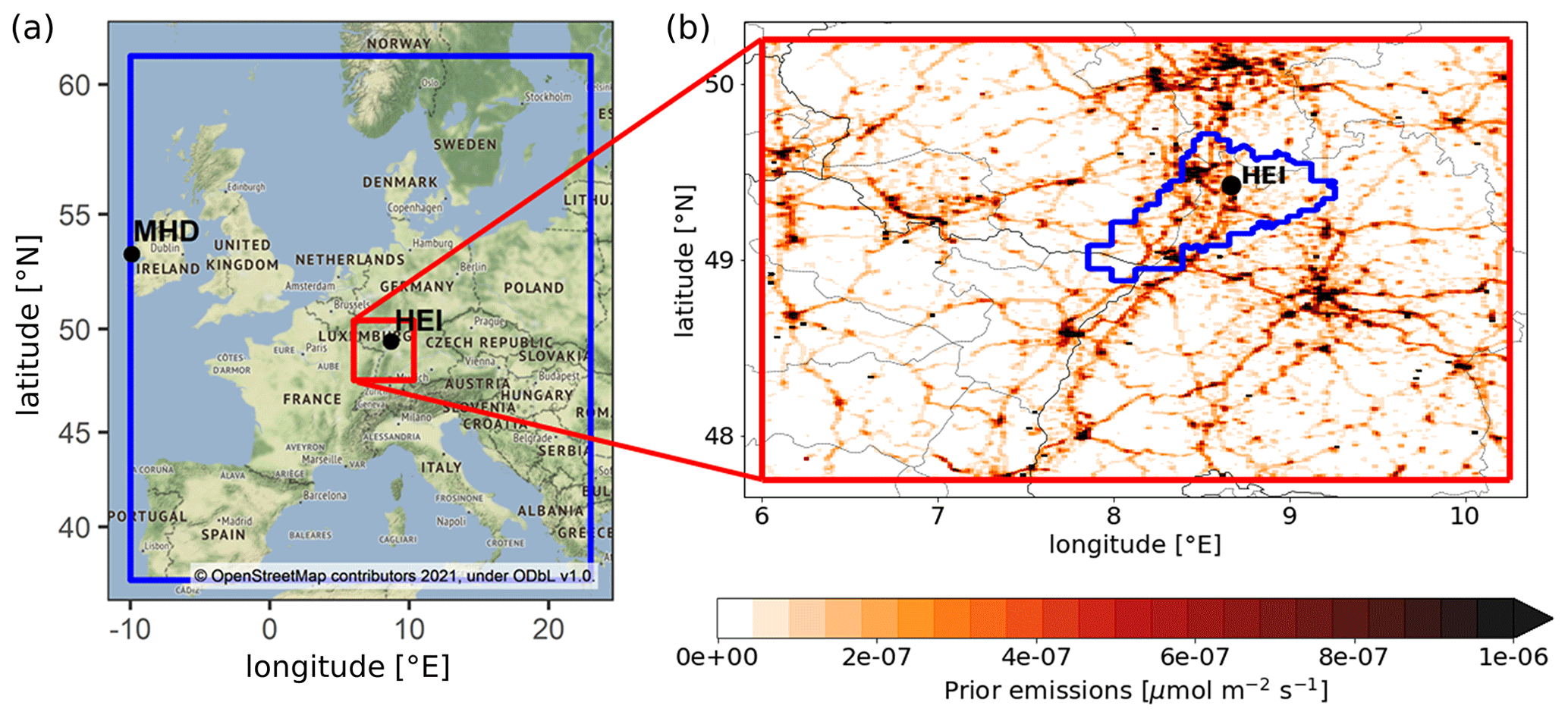
Figure 1 (a) Map of the central European STILT domain (blue) and the high-resolution Rhine Valley STILT domain (red). The Heidelberg (HEI) observation site and the Mace Head (MHD) marine site, which we used as a background site to calculate the ΔffCO₂ concentrations at Heidelberg (see Sect. 2.2.3), are indicated. (b) Zoomed view of the Rhine Valley domain showing the mean prior ffCO₂ emissions from the TNO inventory for 2019–2020. The blue outline within panel (b) shows the “50 % footprint” range, i.e., the area accounting for 50 % of the Heidelberg average footprint within the Rhine Valley.

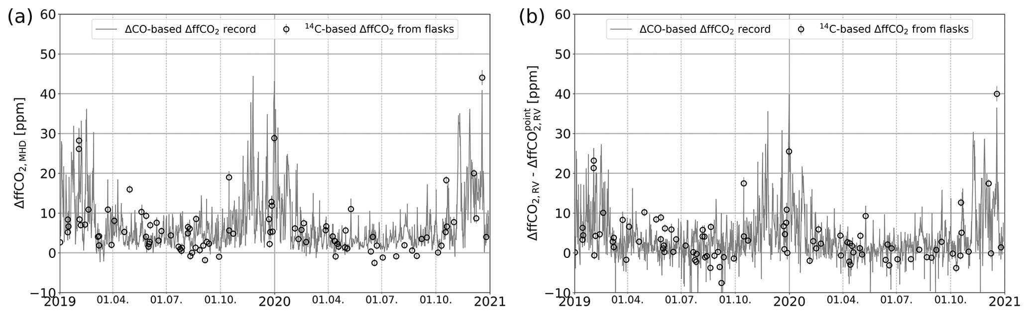
Figure 2 Afternoon ΔffCO₂ observations from the Heidelberg observation site. The gray curve indicates the ΔCO-based ΔffCO₂ record and the black circles show the ¹⁴C-based ΔffCO₂ estimates from flasks. Both the ¹⁴C-based and ΔCO-based ΔffCO₂ observations are 2σ-selected. Panel (a) shows the ΔffCO₂ excess compared with the Mace Head marine background site (i.e., ΔffCO_2,MHD in Eq. 1). Panel (b) shows the ΔffCO₂ excess compared with the Rhine Valley (RV) boundary (i.e., ΔffCO_2,RV in Eq. 1) minus the modeled ΔffCO_2,RV contributions from point sources within the Rhine Valley (ΔffCO${}_{\mathrm{2},\mathrm{RV}}^{\mathrm{point}}$). The data in panel (b) are effectively used to optimize the area source emissions in the Rhine Valley.

The CarboScope inversion system uses Bayesian inference to minimize the deviations between observed and modeled ΔffCO₂ concentrations by finding the (global) minimum of the cost function (for technical details, see Appendix A and Rödenbeck, 2005). This cost function consists of a data constraint and an a priori flux constraint, which is needed to regularize the underdetermined problem and to prevent large and unrealistic spatiotemporal ffCO₂ flux variabilities (Rödenbeck et al., 2018). The data constraint is weighted by the uncertainties of the transport model and the ΔffCO₂ observations. Furthermore, the uncertainty applied for the a priori ffCO₂ emissions determines the impact of the a priori constraint. Overall, the ratio between the model–data uncertainty and the a priori flux uncertainty controls the strength of the a priori constraint over the observational constraint (Rödenbeck, 2005; Kountouris et al., 2018; Munassar et al., 2022). The cost function is minimized by using a conjugate gradient algorithm with reorthogonalization after each iteration step (Rödenbeck, 2005). In this study, we optimize a single scalar on the a priori ffCO₂ emissions field inside the Rhine Valley domain every day.

2.2.1 Atmospheric transport model

We use the Stochastic Time-Inverted Lagrangian Transport (STILT; Lin et al., 2003; Nehrkorn et al., 2010) model, driven by meteorological fields from the high-resolution Weather Research and Forecasting (WRF) model (version 3.9.1.1; Skamarock et al., 2008), to simulate the atmospheric transport in the Rhine Valley domain (see the red rectangle in Fig. 1). Hourly 0.25° resolution data from the fifth generation (ERA5; Hersbach et al., 2020) of the European Centre for Medium-Range Weather Forecasts (ECMWF) atmospheric reanalysis were used as boundary conditions for the WRF simulations. The WRF meteorological fields have a horizontal resolution of 2 km and were generated by applying the MYNN (Mellor–Yamada–Nakanishi–Niino; Nakanishi and Niino, 2009) planetary boundary layer (PBL) parameterization scheme. Finally, using STILT, we calculated the sensitivity of the Heidelberg observations to ffCO₂ emissions from individual grid cells in the catchment area of the site (i.e., the so-called footprint in units of concentration per flux density) by computing the back-trajectories of 100 particles released from the Heidelberg receptor site for each hour. The hourly resolution footprints have a horizontal spatial resolution of about 1 km × 1 km ($\mathrm{1}/\mathrm{60}\mathit{°}\times \mathrm{1}/\mathrm{120}\mathit{°}$, long × lat). As there are many point source emissions within the Rhine Valley, we apply the STILT volume source influence (VSI) approach introduced by Maier et al. (2022) to model them. This modeling approach considers the effective heights (including plume rise) of the point source emissions, which are typically released from elevated chimney stacks. This approach substantially improved the simulation of ΔffCO₂ concentrations at the Heidelberg site, especially during situations with low PBL heights (Maier et al., 2022). For the area source emissions, we apply the standard approach in STILT, which assumes that all emissions are released from the surface.

2.2.2 A priori information

We use the ffCO₂ emissions from the Netherlands Organization for Applied Scientific Research (TNO; Dellaert et al., 2019; Denier van der Gon et al., 2019) with a horizontal resolution of about 1 km ($\mathrm{1}/\mathrm{60}$° $\times \mathrm{1}/\mathrm{120}$°, long × lat) as a priori estimates for our Rhine Valley inversion. The TNO emission inventory provides annual ffCO₂ emissions for 15 different source sectors as well as sector-specific temporal profiles. In this study, we treat the ffCO₂ emissions from the point-source-dominated “energy production” and “industry” TNO sectors separately for the following reasons:

1. While the VSI approach (see above) strongly improves the vertical representation of point source emissions in STILT (Maier et al., 2022), it still remains difficult to correctly describe the mixing and transport of narrow point source plumes with meteorological fields that have a resolution of 2 km.

2. Due to the elevated release of point source emissions from high stacks, the Heidelberg observation site, with an air intake height of only 30 m above the ground, is rarely influenced by distinct emission plumes from nearby point sources (see Fig. 4 in Maier et al., 2024, which shows the $\mathrm{\Delta }\mathrm{CO}/\mathrm{\Delta }{\mathrm{ffCO}}_{\mathrm{2}}$ ratio analysis). This makes it difficult to evaluate those point source emissions with ΔffCO₂ observations from the Heidelberg observation site alone.

3. As the energy and industry point source emissions in TNO are directly based on the European Pollutant and Transfer Register (E-PRTR) database, which provides information on the location and emission of the major facilities in Europe (Kuenen et al., 2014), we expect them to be better known than the more diffuse area source emissions in the Rhine Valley.

Thus, we focus on how well our observations are able to constrain area source emissions in the footprint of the Heidelberg site.

Hence, we prescribe the energy and industry emissions in our inversion setup and adjust only the area source emissions in the Rhine Valley, which mainly originate from the heating and traffic sector. TNO provides monthly profiles for the ffCO₂ emissions from each of the 15 source sectors. We use the monthly profiles for 2019, which are European averages and, thus, identical for all countries within the central European STILT domain (see blue box in Fig. 1a). For 2020, TNO provides country-specific temporal profiles to account for the large variabilities in the length and intensity of the COVID-19 restrictions among the individual countries. As Germany and France are both part of the Rhine Valley domain, we decided to use the average of the German and French temporal profiles for 2020 to construct suitable sector-specific monthly profiles for the Rhine Valley domain in 2020. For all inversion runs performed in this study, we use these TNO monthly profiles to calculate monthly ffCO₂ emissions for the energy and industry sectors from the corresponding annual total emissions.

In this study, we aim to evaluate the ΔffCO₂ observation information regarding the seasonal cycle of the area source ffCO₂ emissions. That is why we apply temporally constant (“flat”) a priori ffCO₂ emissions for the area sources in our standard inversion runs. For this, we use the (high-spatial-resolution) 2-year average TNO area source emissions of the years 2019 and 2020. Finally, we also perform a sensitivity inversion run, in which we replace the temporally flat a priori area source emissions by monthly varying a priori area source emissions. For this, we use the monthly profiles from TNO described above (i.e., the European average monthly profiles in 2019 and the mean of the German and French monthly profiles in 2020) for both the area and the point source emissions.

2.2.3 Observations

In separate inversion runs, we use either the discrete ¹⁴C-based ΔffCO₂ estimates from flasks, collected as integrals over 1 h, or the hourly ΔCO-based ΔffCO₂ record from the Heidelberg observation site (see Fig. 2). The companion paper (Maier et al., 2024) describes the calculation of the ¹⁴C-based ΔffCO₂ estimates in detail as well as the construction of the continuous ΔCO-based ΔffCO₂ record. In short, the ΔCO-based ΔffCO₂ record has been constructed by dividing the continuously measured hourly ΔCO offsets compared with the Mace Head (MHD) marine reference site by an average $\mathrm{\Delta }\mathrm{CO}/\mathrm{\Delta }{\mathrm{ffCO}}_{\mathrm{2}}$ ratio of 8.44±0.07 ppb ppm⁻¹, which was determined from ΔCO and ¹⁴C-based ΔffCO₂ observations of almost 350 daytime and nighttime flask samples collected in 2019 and 2020. Correlation of these ΔCO and ΔffCO₂ values showed only small variability, because heating and traffic $\mathrm{CO}/{\mathrm{ffCO}}_{\mathrm{2}}$ emission ratios in the footprint of Heidelberg are currently very similar (around 8 ppb ppm⁻¹). In the inversion, however, we only use the afternoon ¹⁴C-based and ΔCO-based ΔffCO₂ observations between 11:00 and 16:00 UTC, as nighttime situations are associated with a poorer transport model performance. Times for the hourly integrated ΔffCO₂ observations are reported as the start of the hour, e.g., 11:00 UTC corresponds to the time period between 11:00 and 12:00 UTC. The average uncertainties of the ¹⁴C- and ΔCO-based ΔffCO₂ concentrations were estimated to 1.1 and 3.9 ppm, respectively (Maier et al., 2023a, 2024).

Furthermore, we apply a 2σ-selection criterion to the ΔffCO₂ observations, as introduced by Rödenbeck et al. (2018). For this, we take the high-resolution annual total ffCO₂ emissions from TNO and apply the hourly sector-specific temporal profiles. These hourly resolution ffCO₂ emissions are then transported with the WRF-STILT model to simulate hourly ΔffCO₂ concentrations. The mean difference between the simulated and the ΔCO-based ΔffCO₂ observations is only −0.04 ppm during afternoon hours with a standard deviation of 6.76 ppm (i.e., almost 100 % of the mean value), which indicates that the model is able to reproduce, on average, the afternoon ΔCO-based ΔffCO₂ observations without a significant mean bias. This directly allows the application of the 2σ-selection criterion, which means that we only use those ΔffCO₂ observations whose deviation from the modeled ΔffCO₂ is smaller than 2 times the standard deviation between the observed and modeled ΔffCO₂ (i.e., within the 2σ range). Therewith, we exclude the data outside the 2σ range, which obviously cannot be represented with our transport model. Examples of such data are observations during very strong air stagnation events in winter, which are often underestimated in the model, or, vice versa, situations when the model overestimates the point source influence at the observation site. As the inversion system assumes a Gaussian distribution for the model–data mismatch, these extreme outlier events would have a strong impact on the inversion results (Rödenbeck et al., 2018). Thus, this 2σ-selection criterion can be seen as an additional regularization for the inversion to avoid using situations with unrealistic model simulations. We apply the 2σ-selection criterion to both the ¹⁴C-based ΔffCO₂ observations from the afternoon flask samples and the afternoon hours of the ΔCO-based ΔffCO₂ record.

2.2.4 Lateral boundary conditions

We set up the inversion system for the Rhine Valley domain (47.75–50.25° N, 6.00–10.25° E; red rectangle in Fig. 1a) around the Heidelberg observation site and run the inversion for the full 2 years (2019 and 2020) within this domain. However, as we calculated the ¹⁴C- and ΔCO-based ΔffCO₂ excess compared with MHD (see Maier et al., 2024), we need to define a suitable ΔffCO₂ background representative of the boundary of the Rhine Valley domain. In the following, we call this the “Rhine Valley ΔffCO₂ background”. By definition, we assume that the Δ¹⁴CO₂ observations from MHD correspond to ΔffCO₂=0 ppm, which is reasonable because the MHD ¹⁴CO₂ samples were only collected during situations with clean westerly air masses from the Atlantic. Therefore, it seems to be suitable to apply the MHD (ΔffCO₂=0 ppm) background to the entire western boundary of the central European STILT domain (blue rectangle in Fig. 1a). However, this introduces the following question: “How representative is this background of the other boundaries of the central European domain?”. Maier et al. (2023a) estimated the representativeness bias of the MHD background for the eastern boundary of the central European domain, which is likely the most polluted border. They showed that the representativeness bias is on average smaller than 0.1 ppm for an observation site in central Europe. Therefore, we neglect this bias and also assume ΔffCO₂=0 ppm at the non-western boundaries of the central European domain. To estimate the Rhine Valley ΔffCO₂ background, we then use a nested STILT model approach with a 2 km horizontal resolution WRF meteorology in the Rhine Valley domain and a coarser (10 km) WRF resolution in the central European STILT domain outside the Rhine Valley. For both domains, we use hourly ffCO₂ emissions from TNO (Dellaert et al., 2019; Denier van der Gon et al., 2019). This nested approach allows us to separate the ffCO₂ contributions from each STILT domain. With this setup, we model the ΔffCO₂ contributions from the central European domain outside the Rhine Valley (ΔffCO_2,CE-RV) for the Heidelberg site for each hour during 2019 and 2020. We then subtract this modeled Rhine Valley ΔffCO₂ background (ΔffCO_2,CE-RV) from the estimated ΔffCO₂ excess compared with MHD (ΔffCO_2,MHD) to obtain the ΔffCO₂ excess compared with the Rhine Valley boundary (ΔffCO_2,RV):

$$\begin{array}{}\text{(1)}& \mathrm{\Delta }{\mathrm{ffCO}}_{\mathrm{2},\mathrm{RV}}=\mathrm{\Delta }{\mathrm{ffCO}}_{\mathrm{2},\mathrm{MHD}}-\mathrm{\Delta }{\mathrm{ffCO}}_{\mathrm{2},\mathrm{CE}\text{-}\mathrm{RV}}.\end{array}$$

The ΔffCO_2,RV excess concentrations compared with the Rhine Valley boundary are then introduced into the inversion system to constrain the ffCO₂ emissions within the Rhine Valley. Note, however, that the actual data constraint is the ΔffCO_2,RV excess minus the modeled ΔffCO₂ contribution from the point sources within the Rhine Valley (ΔffCO${}_{\mathrm{2},\mathrm{RV}}^{\mathrm{point}}$; see Fig. 2b), as we prescribe the point source emissions and only optimize for the area source emissions.

We also want to emphasize that the ΔffCO_2,RV excess concentrations rely on the STILT transport and the TNO emissions being correct. A potential bias in the modeled transport or the ffCO₂ emissions outside the Rhine Valley would directly translate into a bias in the ΔffCO_2,RV excess concentrations. This, in turn, might affect the deduced ffCO₂ fluxes within the Rhine Valley domain. To assess the impact of the Rhine Valley ΔffCO₂ background (ΔffCO_2,CE-RV) on the a posteriori ffCO₂ fluxes in the main footprint of Heidelberg, we also perform an inversion run with an alternative Rhine Valley ΔffCO₂ background. We again model this alternative background with STILT but apply the 0.25° resolution forecasting meteorological data from the Integrated Forecasting System (IFS) instead of the WRF meteorology (see Sect. 2.2.1). Moreover, we replace the TNO emissions with the Emissions Database for Global Atmospheric Research (EDGAR, version 4.3.2; Janssens-Maenhout et al., 2019) emissions to prescribe the ffCO₂ fluxes in Europe. This EDGAR inventory was updated to the years 2019 and 2020 by taking the British Petroleum (BP) statistics on fossil fuel consumption into account and was remapped on a grid with a horizontal resolution of 0.25°. Note that we only use this coarser STILT resolution for simulating the alternative Rhine Valley ΔffCO₂ background. The inversion itself is again performed with the high-resolution WRF meteorology (see Sect. 3.3).

2.2.5 Model–data mismatch

The model–data mismatch (MDM) is calculated by subtracting the modeled from the observed ΔffCO_2,RV concentrations. The uncertainties of the ΔCO-based and ¹⁴C-based ΔffCO₂ observations are estimated to be 3.9 and 1.1 ppm, respectively (see Maier et al., 2024). The transport model uncertainty of urban, continental sites like Heidelberg with complex local circulations was assumed to be 5 ppm. The quadratically added observational and transport model uncertainties yield the total uncertainty of the model–data mismatch, which we call the MDM error in the following. To account for the temporal correlations of observations that are close together in time, we apply a data density weighting, as described in Rödenbeck (2005). It artificially increases the MDM error, so that all observations within 1 week lead to the same constraint as a single observation per week. The weighting interval was set to 1 week because this is a typical duration of synoptic weather patterns. Depending on the number of observations per week, the final MDM error of individual hourly observations ranges between 5.1 and 7.8 ppm in the case of ¹⁴C-based ΔffCO₂ from flasks and between 23.7 and 37.5 ppm in the case of the ΔCO-based ΔffCO₂ record.

Based on our analysis results presented in Sect. 3.1, we decided to apply weekly averaging in the case of the ΔCO-based ΔffCO₂ inversion (see Sect. 3.2), which we briefly describe here. The MDM vector for the ΔCO-based ΔffCO₂ inversion has a length of 3237, which represents the number of the (2σ-selected) afternoon hours with available ΔCO-based ΔffCO₂ observations. Weekly averaging means that each hourly entry of the MDM vector within a week is replaced by the respective weighted average MDM of that week. The weight of the individual hours within a week is defined by the MDM error of the respective hours. This means that the weekly averaged MDM vector has the same length as the original MDM vector. We do not modify the hourly MDM errors when applying the weekly averaging. This means that the weekly averaging would not change anything if all hourly MDM entries within a week were initially (by chance) the same.

2.2.6 Degrees of freedom

As we only use ΔffCO₂ observations from one single station in the Rhine Valley, we restrict the number of degrees of freedom in our inversion system so that the inverse problem is not too strongly underdetermined. Therefore, we only investigate the area source emissions in the Rhine Valley and prescribe the energy and industry emissions, as described above. Moreover, the inversion system adjusts only one spatial scaling factor per day, which increases or decreases the area source emissions in the whole Rhine Valley domain equally. Hence, we expect that the high-resolution TNO inventory is much better at describing the large spatial heterogeneity in the ffCO₂ emissions within the Rhine Valley than our top-down approach. As we want to investigate the seasonal cycle of the ffCO₂ emissions, additional temporal degrees of freedom are needed. For this, we choose a temporal correlation length of about 4 months (“Filt3T” in CarboScope notation), which should be appropriate to explore seasonal cycles. Finally, because the Heidelberg observations cannot be used to constrain the emissions in the whole Rhine Valley domain, we only analyze the a posteriori area source emissions in the (most constrained) near field of the observation site. We define the near field of Heidelberg as the area that accounts for 50 % of the temporally accumulated footprint in the Rhine Valley domain for the 2 years of 2019 and 2020 (blue outlined region in Fig. 1b).

3 Results

3.1 Potential of flask-based ΔffCO₂ estimates to investigate the seasonal cycle of ffCO₂ emissions

First, we investigate the potential of flask-based ΔffCO₂ estimates to resolve the seasonal cycle of the area source ffCO₂ emissions around the urban Heidelberg observation site. For this, we use the average of the TNO area source ffCO₂ emissions of the 2 years of 2019 and 2020 as a temporally constant prior estimate (see Sect. 2.2.2). To analyze the impact of the observational constraint on the a posteriori results, we apply different prior uncertainties, which effectively lead to different ratios between a priori and observational constraints (Fig. 3). In a first inversion run (Fig. 3a), we use the ¹⁴C-based ΔffCO₂ observations from the 94 afternoon flasks collected in Heidelberg in the 2 years of 2019 and 2020. The distribution of the flask samplings over the 2 years can be seen in Fig. 2. For various reasons (e.g., testing of the flask sampler associated with frequent changes in the flask sampling strategy), the flasks were not evenly collected; specifically, the 2019–2020 winter has only limited flask coverage. The ¹⁴C-based a posteriori ffCO₂ emissions show a clear seasonal cycle for the larger prior uncertainties that is mainly data-driven. However, large and unrealistic a posteriori flux variabilities emerge for prior uncertainties larger than 50 % of the flat a priori emissions. For example, the low flask coverage during the 2019–2020 winter period leads to a huge maximum in the area source ffCO₂ emissions in November 2019 when the inversion algorithm tries to fit individual flask observations that have large model–data mismatches (see Fig. B1). Similarly, the flask samples in summer 2020 with near-zero or even negative ΔffCO₂ estimates, which lead to negative model–data mismatches (cf. Figs. 2b and B1), cause a strong reduction in the a posteriori emissions.

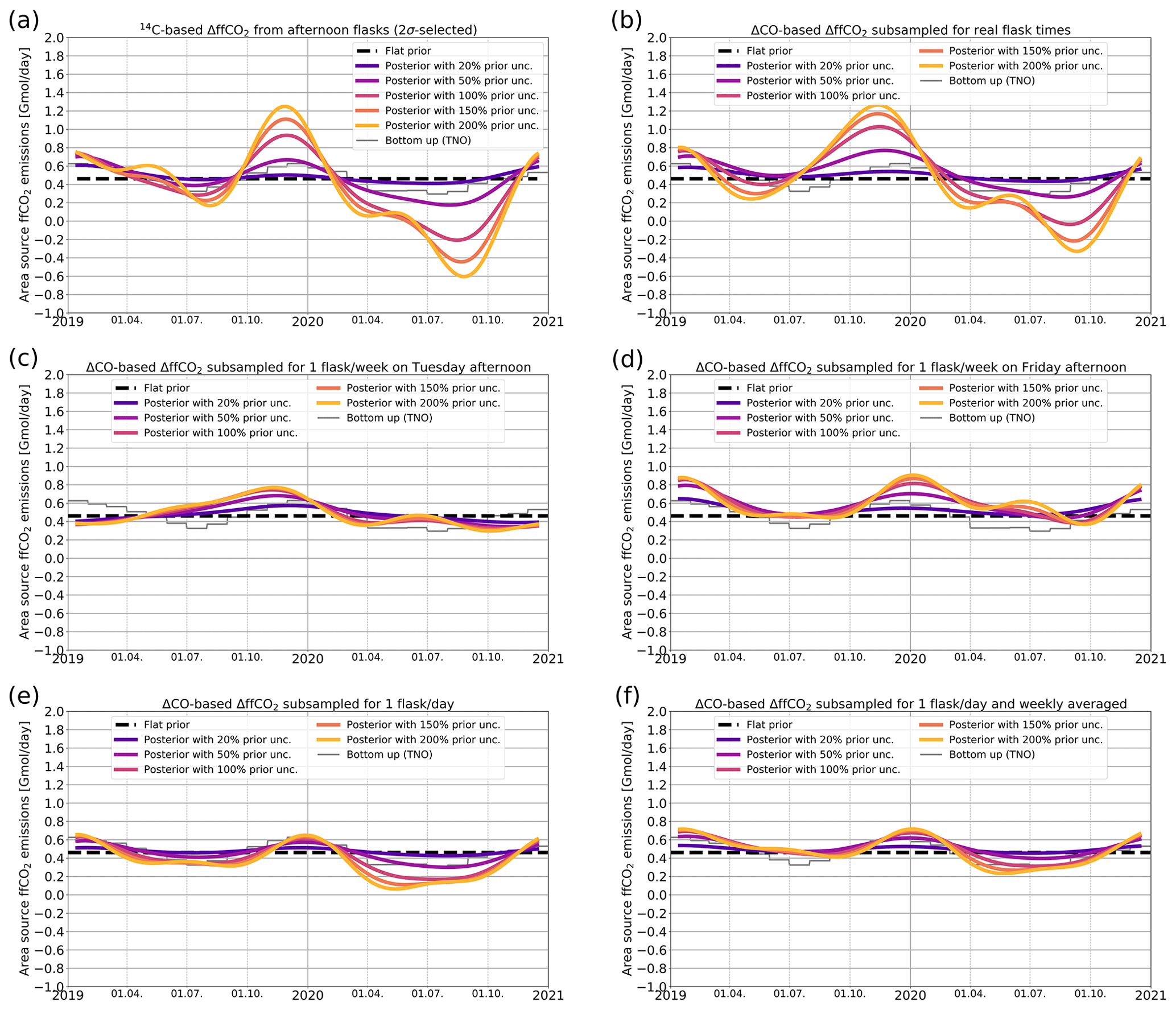
Figure 3 Area source ffCO₂ emissions in the near field (blue outlined area in Fig. 1b) of Heidelberg. Shown are the flat prior emissions (dashed black line), the a posteriori emissions for different prior uncertainties between 20 % and 200 % of the flat a priori emissions (solid colored lines) as well as the bottom-up estimates from TNO (gray line). In panel (a), ¹⁴C-based ΔffCO₂ estimates from 94 2σ-selected afternoon flasks from Heidelberg were used as observational input (see Fig. 2). Panel (b) shows the inversion results if the ΔCO-based ΔffCO₂ observations subsampled during the 94 flask sampling hours were used. In panels (c) and (d), the inversion was constrained with one hourly afternoon (at 13:00 UTC) ΔCO-based ΔffCO₂ observation every week collected on the 2 random working days of Tuesday (c) or Friday (d). Panel (e) shows the results if one hypothetical flask is collected each day at 13:00 UTC. In panel (f), the seven afternoon flask observations within 1 week are averaged.

Figure B1 shows the agreement between the flat prior and the different a posteriori-based model results and the flask observations. The flat prior emissions lead to a mean bias (observed minus modeled ΔffCO₂ concentration) of 0.68 ppm with a standard deviation of 5.61 ppm. The a posteriori emissions based on a 50 % prior uncertainty reduce the mean bias and the standard deviation to 0.35±5.23 ppm. However, for higher prior uncertainties, the mean bias increases again and only the standard deviation is further reduced; for example, a prior uncertainty of 150 % leads to a mean bias of 0.54±4.78 ppm between the observed and modeled ΔffCO₂ concentration. This might be an indication of overfitting. To further investigate the performance of the inversion, we conducted a reduced chi-square (${\mathit{\chi }}_{\mathrm{r}}^{\mathrm{2}}$) analysis. The ${\mathit{\chi }}_{\mathrm{r}}^{\mathrm{2}}$ values decrease from 1.10 (for a 50 % prior uncertainty) to 0.97 (for a 150 % prior uncertainty). Typically, ${\mathit{\chi }}_{\mathrm{r}}^{\mathrm{2}}$ values smaller than 1 are an indication of overfitting if the model–data mismatch error is chosen properly. However, as the ${\mathit{\chi }}_{\mathrm{r}}^{\mathrm{2}}$ values (for prior uncertainties between 50 % and 200 %) are all close to 1 (within ±10 %), the ${\mathit{\chi }}_{\mathrm{r}}^{\mathrm{2}}$ values might not be suitable to demonstrate overfitting in our case. Overall, this urban inversion setup obviously needs a very strong regularization through low prior uncertainties to prevent the fitting of individual flask observations and, thus, unrealistic variability in the a posteriori ffCO₂ emissions. This indicates that the applied 2σ-filtering approach (see Sect. 2.2.3) is not sufficient in this urban setting.

We further investigate whether these overfitting patterns can be attributed to the uneven distribution of the flask samples. For this, we subsample the continuous ΔCO-based ΔffCO₂ record. In a first step, we use the ΔCO-based ΔffCO₂ observations from those 94 afternoon hours with flask samples as an observational constraint (Fig. 3b). For the most part, the subsampled ΔCO-based ΔffCO₂ observations reproduce the a posteriori results of the ¹⁴C-based ΔffCO₂ estimates. However, there are differences, like the shifted summer minimum in 2019. These differences can be explained by the deviations between the ¹⁴C-based and ΔCO-based ΔffCO₂ estimates in Fig. 2, and thus the variability in the $\mathrm{\Delta }\mathrm{CO}/\mathrm{\Delta }{\mathrm{ffCO}}_{\mathrm{2}}$ ratios that we fully neglected by using a constant mean ratio for constructing the ΔCO-based ΔffCO₂ record. Therefore, when comparing the results with the TNO seasonality of emissions (gray histogram), it seems obvious that the ¹⁴C-based ΔffCO₂ estimates provide more accurate data than the subsampled ΔCO-based ΔffCO₂ record. However, the general similarity between both results means that we can use the continuous ΔCO-based ΔffCO₂ record to investigate an even data coverage with hypothetical Heidelberg flask samples. Figure 3c and d show the inversion results if the ΔCO-based ΔffCO₂ record is subsampled for one flask every week on Tuesday or on Friday afternoon, respectively. We chose Tuesday and Friday as random examples of 2 working days. The evenly distributed weekly flasks strongly dampen the variability in the a posteriori results. However, they show large differences depending on which day of the week the hypothetical afternoon flask was collected: whereas the Tuesday flasks lead to a quite unrealistic gradual increase in the ffCO₂ emissions between January and November 2019, the Friday flasks show a more realistic seasonal cycle in this year. In contrast, both Tuesday and Friday flasks lead to an unexpected maximum in summer 2020. The comparison between the (hypothetical) flask concentrations and the a posteriori results illustrates again that the inversion mainly tries to fit those individual hours with the largest MDM (not shown). This implies that the a posteriori results are still dependent on the selection of the individual hypothetical flasks. Therefore, it seems that even a uniform data coverage with a realistic flask sampling frequency of one flask per week is not sufficient to determine a plausible seasonal cycle of the area source ffCO₂ emissions around Heidelberg (as, e.g., suggested by the TNO inventory). However, the situation should be improved in the case of real, hourly integrated ¹⁴C flasks that are collected, e.g., once per week, as the average $\mathrm{\Delta }\mathrm{CO}/\mathrm{\Delta }{\mathrm{ffCO}}_{\mathrm{2}}$ ratio used to construct the ΔCO-based ΔffCO₂ record might be inappropriate for individual hours.

Finally, we investigated the benefit of an extremely high flask sampling frequency of one flask per afternoon (see Fig. 3e). Note that such a high-frequency flask sampling increases the MDM error because of the applied data density weighting (see Sect. 2.2.5). Here, the a posteriori results seem to approach the TNO bottom-up emissions in 2019. However, there are still unexpectedly strong deviations between the top-down and bottom-up estimates in the summer half-year of 2020 for increased prior uncertainties. These differences might be caused by individual afternoon hours with a negative MDM in summer 2020. To reduce the impact of such hours, we perform a separate inversion run in which we average the modeled and observational data of all seven hypothetical afternoon flasks within each week (Fig. 3f; see Sect. 2.2.5 for a description of the weekly averaging of the MDM vector). This further reduces the spread of a posteriori results, particularly in summer 2020, further approaching the seasonal amplitude of the bottom-up TNO emissions. Thus, several afternoon flasks per week would be needed so that the influence of individual flasks on the inversion results can be averaged out and a plausible seasonal cycle amplitude in the area source ffCO₂ emissions around Heidelberg can be obtained.

Overall, these results show that the a posteriori estimates are very sensitive to individual flask observations in the Heidelberg target region, which has very heterogeneously distributed ffCO₂ sources. Obviously, the transport model fails to appropriately simulate the ΔffCO₂ concentrations for individual afternoon hours. This can be explained by remaining shortcomings in the transport model as well as by the enormous heterogeneity in the ffCO₂ emissions in the footprint of the Heidelberg observation site. As already mentioned in Sect. 2, modeling individual plumes from point source emissions is a particular challenge in this urban region, and, for example, the forward model estimates of point source signals, even with the improved VSI approach, often seem incorrect, at least at a temporal resolution of 1 h. Moreover, there might also be inaccuracies in the TNO point source emissions themselves. Finally, part of the MDM can also be explained by uncertainties in the proxies used to spatially disaggregate the area source emissions in the TNO inventory (Super et al., 2020).

3.2 Potential of continuous ΔCO-based ΔffCO₂ estimates to investigate the seasonal cycle of ffCO₂ emissions

The big advantage of the continuous ΔCO-based ΔffCO₂ record is that it provides full temporal coverage of the inversion period and can, thus, also be averaged such that the sensitivity of the a posteriori results to individual (hourly) model–data mismatches with poor model performance is strongly reduced. In Appendix C, we investigate the time interval over which the hourly ΔCO-based and modeled ΔffCO₂ concentrations should be averaged to sufficiently reduce the impact of the point source emissions on the a posteriori area source emissions. For this, in addition to the standard inversion runs with fixed point source emissions, we perform further sensitivity runs with adjustable point source emissions. Ideally (i.e., if the point source emissions are well described in TNO), the a posteriori area source emissions are identical for both inversion runs, meaning that the modeling of the better-known point source emissions has no impact on the area source emissions. It turns out that the averaging interval of 1 week strongly reduces the impact of the point sources on the a posteriori area source emissions (see blue curves in Fig. C1). It limits the differences between the a posteriori area source emissions of the inversion runs with fixed and adjustable point source emissions to below 30 % for individual seasons. Averaged over the 2 years (2019 and 2020), these differences are below 10 %. Therefore, for the ΔCO-based ΔffCO₂ inversion, we apply weekly averaging to the MDM vector (as described in Sect. 2.2.5).

In the following, we use the weekly averaged afternoon ΔCO-based ΔffCO₂ observations to investigate the seasonal cycle of the area source ffCO₂ emissions around Heidelberg (see Fig. 4a). If the chosen prior uncertainty is large enough, the seasonal cycle amplitude of the a posteriori estimates agrees with that of the TNO inventory reasonably well. Moreover, the data-driven inversion results distinctly show the effect of the COVID-19 restrictions, with lower emissions in 2020 compared with 2019. In southwestern Germany, the first COVID-19 lockdown started in mid-March 2020. Indeed, the inversion results show a strong decrease in the area source ffCO₂ emissions at that time. In particular, the decline in the a posteriori ffCO₂ emissions is much steeper in spring 2020 than in spring 2019 and the minimum of the seasonal cycle is flatter in 2020 (as it extends over several summer months). The sharp drop in emissions at the beginning of the COVID-19 restrictions in spring 2020 can also be seen in Fig. D1, where we plot the difference between the seasonal cycles of the 2 years.

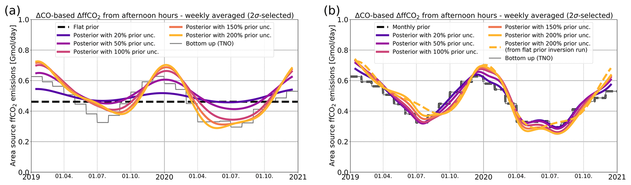
Figure 4 Area source ffCO₂ emissions in the near field (blue outlined area in Fig. 1b) of Heidelberg. In panel (a), a flat prior (dashed black line) was used for the area source emissions; in panel (b), a monthly prior, i.e., the monthly bottom-up estimates from TNO (dashed gray line), was used as the a priori estimate. Shown are the a posteriori emissions for different prior uncertainties between 20 and 200 % (solid colored lines). The inversion was constrained with weekly averages of hourly, 2σ-selected afternoon ΔCO-based ΔffCO₂ observations from Heidelberg. For comparison, the posterior emissions with 200 % prior uncertainty from panel (a) are shown as a dashed yellow line in panel (b).

The agreement with the phasing of the seasonal cycle of the TNO inventory seems to be better in 2020 than in 2019. As described in Sect. 2.2.2, TNO provides country-specific “COVID-19” time profiles for 2020 that consider the timing and the strength of the respective national restrictions. For this year, Fig. 4 shows the average of the monthly time profiles from Germany and France applied to the annual Rhine Valley emissions (gray histogram). This seasonal cycle for 2020 seems to be confirmed by our observations. However, the TNO seasonal cycle shown for 2019 is a general estimate constructed for the whole central European domain (see Fig. 1) that is neither specific for individual countries nor for the year 2019. It assumes minimum emissions in July, whereas our observations show minimum emissions in August and September. Indeed, this shifted minimum of the seasonal cycle coincides with the summer holidays in southwestern Germany, which are from August to mid-September.

We further investigate the consistency of the seasonal cycles from the bottom-up and the top-down estimates. For this, we explore the effect of using the monthly TNO bottom-up seasonal cycle for the a priori emissions (see Fig. 4b). As expected, the phase of the a posteriori seasonal cycle is in agreement with the TNO inventory in 2020. However, the a priori information pulls the summer emission minimum to July in 2019. With weakening regularization of the prior, the inversion algorithm tries to shift the minimum of the a posteriori seasonal cycle from July towards August and September. Due to the limited temporal degrees of freedom of the inversion, this shifting artificially increases the emissions in May 2019 and lowers them in October. Hence, these results might point to some inconsistencies in the seasonality of the TNO emissions in the main footprint of the Heidelberg observation site. In fact, correct phasing of the fossil emissions is essential when prescribed ffCO₂ emissions are used in CO₂ model inversions to separate the fossil from the biogenic contribution in atmospheric CO₂ observations and constrain CO₂ fluxes from the biosphere. Although these biospheric CO₂ signals are typically estimated with observations from sites that are more remote and rural than the urban Heidelberg site, the correct seasonality in prescribed ffCO₂ emissions is still important when deducing the month-to-month variations in the biospheric CO₂ fluxes.

Overall, the (weekly averaged) ΔCO-based ΔffCO₂ record seems to be well suited to estimate (and validate) the seasonal cycle of bottom-up ffCO₂ emissions in the near field of the Heidelberg observation site. This is a very promising result, especially considering how simply the ΔCO-based ΔffCO₂ record was constructed. It is based on the 2-year average $\mathrm{\Delta }\mathrm{CO}/\mathrm{\Delta }{\mathrm{ffCO}}_{\mathrm{2}}$ ratio estimated from ¹⁴C measurements on flask samples, and a potential seasonal cycle in the $\mathrm{\Delta }\mathrm{CO}/\mathrm{\Delta }{\mathrm{ffCO}}_{\mathrm{2}}$ ratios was fully neglected.

3.3 Robustness of the ΔCO-based ΔffCO₂ inversion results

In the following, we investigate the robustness of the (weekly averaged) ΔCO-based ΔffCO₂ inversion results. For this, we (1) reduce the flat prior emissions by 20 %, (2) assume a seasonal cycle in the $\mathrm{\Delta }\mathrm{CO}/\mathrm{\Delta }{\mathrm{ffCO}}_{\mathrm{2}}$ ratios, and (3) apply an alternative Rhine Valley ΔffCO₂ background. In Fig. 5, we show the respective a posteriori results for a prior uncertainty of 150 %, which constitutes enough weighting on the (weekly averaged) ΔCO-based ΔffCO₂ observations to reconstruct the seasonal cycle from the flat a priori area source ffCO₂ emissions (see Fig. 4a). Moreover, the 150 % prior uncertainty reduces the mean bias between the weekly averaged ΔCO-based ΔffCO₂ observations and the a posteriori fits to 0.10±1.89 ppm (compared with the mean bias of 0.65±2.23 ppm, which one gets when using the flat prior emissions). Further increasing the prior uncertainty to 200 % leads to only neglectable changes in the mean bias (0.11±1.88 ppm).

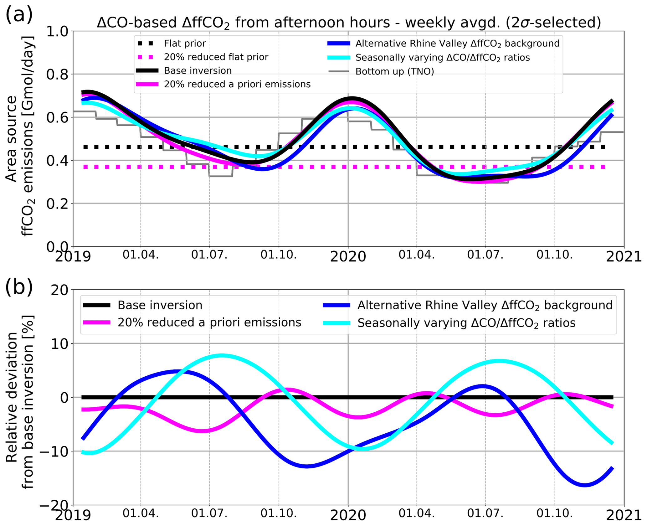
Figure 5 (a) Area source ffCO₂ emissions in the near field (blue outlined area in Fig. 1b) of Heidelberg for different sensitivity runs. Shown are the a posteriori results for a 20 % reduction in the flat a priori emissions (solid magenta line), for an alternative Rhine Valley ΔffCO₂ background modeled with EDGAR emissions (blue), and for an assumed seasonal cycle in the $\mathrm{\Delta }\mathrm{CO}/\mathrm{\Delta }{\mathrm{ffCO}}_{\mathrm{2}}$ ratios (cyan; see Fig. E1). As a reference, the a posteriori result of the base inversion from Fig. 4a is shown in black. All a posteriori results correspond to a 150 % prior uncertainty. The dotted lines indicate the flat prior emissions (black) and the prior emissions reduced by 20 % (magenta). Panel (b) shows the relative deviations between the different a posteriori area source emissions of the sensitivity runs and the base inversion (in %).

First, if the a priori area source ffCO₂ emissions in the Rhine Valley domain are equally reduced by 20 % (see dotted magenta line in Fig. 5a), the ΔCO-based ΔffCO₂ inversion manages to compensate for almost all of this bias (compare the magenta curves with the black curves in Fig. 5). The deviations between the a posteriori emissions of the inversion runs with perturbed and unperturbed flat prior emissions is typically below 5 % for all seasons (Fig. 5b). Accordingly, the a posteriori seasonal cycle of the ffCO₂ emissions is hardly affected by a potential bias in the flat prior emissions. The deviations between the annual totals of the a posteriori estimates of the perturbed and unperturbed prior inversion runs is only 2 % for both years. This means that about 90 % of this 20 % bias in the perturbed flat prior could be corrected for with the observational constraint on an annual scale.

With the second sensitivity test, we want to investigate the effect of the $\mathrm{\Delta }\mathrm{CO}/\mathrm{\Delta }{\mathrm{ffCO}}_{\mathrm{2}}$ ratios used to construct the ΔCO-based ΔffCO₂ record. For our base inversion, the ΔCO-based ΔffCO₂ record was constructed using the average $\mathrm{\Delta }\mathrm{CO}/\mathrm{\Delta }{\mathrm{ffCO}}_{\mathrm{2}}$ ratio of 8.44±0.07 ppb ppm⁻¹, which was calculated from all flask samples collected in Heidelberg in 2019 and 2020. However, as discussed in Maier et al. (2024), the ratio during summer with lower signals is hard to determine and, thus, less constrained. Indeed, the winter flasks show a slightly higher mean $\mathrm{\Delta }\mathrm{CO}/\mathrm{\Delta }{\mathrm{ffCO}}_{\mathrm{2}}$ ratio (8.52±0.08 ppb ppm⁻¹, R²=0.89) compared with the summer flasks (8.08±0.17 ppb ppm⁻¹, R²=0.36). This introduces the following question: “How would our inversion results change if the $\mathrm{\Delta }\mathrm{CO}/\mathrm{\Delta }{\mathrm{ffCO}}_{\mathrm{2}}$ ratios would have a (small) seasonal cycle?”. For this, we assume a seasonal cycle in the ratios for the 2 years, with 5 % lower ratios in the summer half-year and, correspondingly, 5 % larger ratios in the winter half-year; the 2-year mean is still 8.44 ppb ppm⁻¹ (see Fig. E1). Notice that we use the ratios to calculate the ΔffCO_2,MHD excess compared with the MHD background site and then subtract the modeled Rhine Valley ΔffCO_2,CE-RV background to get the ΔffCO_2,RV observations for our Rhine Valley inversion (see Eq. 1). This effectively results in summer and winter ΔffCO₂ concentrations being more than 5 % higher and lower than the ΔffCO₂ concentrations based on the average ratio, respectively. Obviously, this leads to larger a posteriori emissions (cyan curve in Fig. 5) during summer and lower emissions in winter compared with the base inversion results. The largest seasonal deviations from the base inversion a posteriori emissions are 10 %. As, by construction, the mean of the seasonally varying ratios corresponds to the average ratio used for the base inversion, the effect on the annual totals of the a posteriori ffCO₂ emissions is neglectable.

Finally, we investigate the impact of the lateral ΔffCO₂ boundaries on the area source ffCO₂ emissions estimates. For our base inversion, we used the high-resolution TNO emission inventory and WRF-STILT to model (for the Heidelberg observation site) the ΔffCO₂ contributions from the European STILT domain outside the Rhine Valley (see Sect. 2.2.4). For the following sensitivity run (blue curve in Fig. 5), we model the Rhine Valley ΔffCO₂ background with ffCO₂ emissions based on the EDGAR emissions and with a coarser meteorology in STILT (see Sect. 2.2.4). The application of this alternative Rhine Valley ΔffCO₂ background leads to more than 10 % lower emissions in the autumn of both years, which can be explained by strong deviations between the weekly averages of the two modeled background concentrations during these periods (see Fig. F1). Thus, the Rhine Valley background affects the seasonal cycle of the area source ffCO₂ emissions. During summer, the deviations from the base inversion results are below 5 %. The annual totals of the area source ffCO₂ emissions around Heidelberg are 3 % and 7 % lower in the years 2019 and 2020, respectively, if the alternative Rhine Valley ΔffCO₂ background is used.

4 Discussion and conclusions

In the present study, we investigate the potential of ¹⁴C-based and ΔCO-based ΔffCO₂ observations to evaluate the ffCO₂ emissions and their seasonal cycle in an urban region around the Heidelberg observation site. This urban area is characterized by complex topography and large spatial heterogeneity in ffCO₂ sources, including several nearby point sources. Thus, deficits in the transport model as well as inaccuracies in the driving meteorology and the prescribed point source emissions strongly impact the model–data mismatch at the observation site, which will be minimized by the inversion algorithm. We focus on the estimation of the ffCO₂ emissions from area sources, as the observations from the Heidelberg site with an air intake height of 30 m above the ground are not suitable to constrain the emissions of nearby point sources with elevated stack heights. Indeed, the analysis of the $\mathrm{\Delta }\mathrm{CO}/\mathrm{\Delta }{\mathrm{ffCO}}_{\mathrm{2}}$ ratios in Maier et al. (2024) showed that the Heidelberg observation site is hardly influenced by pure point source emission plumes. Moreover, we expect that point source emissions can be better quantified a priori from the bottom up compared with area source emissions. Therefore, we prescribe the better-known point source ffCO₂ emissions in the inversion setup and only adjust the area source emissions in the Rhine Valley domain.

4.1 Can flask-based ΔffCO₂ observations be used to predict the seasonal cycle of ffCO₂ emissions at an urban site?

To investigate the potential of ΔffCO₂ observations to predict the seasonal cycle of the area source ffCO₂ emissions around Heidelberg, we applied temporally constant (flat) a priori ffCO₂ emissions in our inversion system, such that all seasonal information comes from the atmospheric data. We have shown that ¹⁴C-based ΔffCO₂ observations from almost 100 hourly flask samples collected in the 2 years of 2019 and 2020 are not sufficient to reconstruct a robust seasonal cycle from the flat a priori estimate. As the Bayesian inversion setup assumes a Gaussian distribution for the model–data mismatch, the inversion algorithm tries to primarily reduce the largest model–data differences. Therefore, we applied a 2σ-selection criterion to exclude the flask events with the largest model–data mismatches and, thus, poorer model performance. However, the a posteriori ffCO₂ emissions are still very sensitive to individual flask observations. This may suggest that the 2σ filter is not sufficient in a densely populated high-fossil-fuel environment like Heidelberg with a complex topography. Therefore, strong regularization through small a priori uncertainties (i.e., < 50 % prior uncertainty; Fig. 3a) is needed in the case of flask observations to avoid large overfitting patterns in the inversion results.

Due to the fortunate circumstance of currently having similar heating and traffic emission ratios in the main footprint of Heidelberg, we decided to use the 2-year average ¹⁴C-based $\mathrm{\Delta }\mathrm{CO}/\mathrm{\Delta }{\mathrm{ffCO}}_{\mathrm{2}}$ ratio from the flasks to construct a continuous ΔCO-based ΔffCO₂ record (see Maier et al., 2024). By subsampling this ΔCO-based ΔffCO₂ record, we further investigate the potential of uniform data coverage with one hypothetical afternoon flask per week to reliably estimate the seasonal cycle in the area source emissions. Indeed, several afternoon flask samples per week are needed, in addition to an averaging of the flask observations within 1 week so that the overfitting of individual flask data is reduced. However, the situation should be better for real, e.g., sub-weekly, ¹⁴C flasks compared with the subsampled ΔCO-based ΔffCO₂ record. As the applied 2-year average $\mathrm{\Delta }\mathrm{CO}/\mathrm{\Delta }{\mathrm{ffCO}}_{\mathrm{2}}$ ratio may be inappropriate for individual hours, this could amplify the sensitivity to the individual hypothetical flasks.

4.2 What is an appropriate averaging interval for urban observations?

The main advantage of the ΔCO-based ΔffCO₂ record is its continuous data coverage that allows an averaging so that the influence of individual hours with poor model performance on the inversion results is strongly reduced. The comparison of Fig. 3e with Fig. 3f and Fig. 4a clearly illustrates that the averaging of multiple hourly observations leads to a reduction in the a posteriori flux variability. In this urban region, such an averaging is especially necessary because of the shortcomings in the STILT model and its driving meteorology with respect to describing the transport and mixing of nearby point source emissions. Imagine that the plume of a point source arrives at the observation site a few hours earlier or later than simulated by STILT. In such cases, averaging is inevitable in order to prevent the incorrect adjustment of the ffCO₂ emissions. Moreover, the STILT-VSI approach itself has its deficits, as it assumes mean effective emission height profiles for all meteorological situations and ignores the stack heights of individual power plants. Furthermore, the VSI approach still relies on correct vertical mixing in STILT and an accurate point source emission inventory. Although, we could show that the VSI approach strongly improves the agreement between modeled and observed ΔffCO₂ concentrations from 2-week integrated samples in Maier et al. (2022), it may still overestimate the point source contributions for individual hours. Therefore, an averaging of the observations is very helpful when a transport model like STILT is used to describe the transport and mixing of nearby point source emissions.

We investigate how to appropriately average the observational and modeled data. Ideally, the a posteriori area source ffCO₂ emissions are independent of an incorrect modeling of the point source emissions. Thus, they should not be affected by whether the a priori point source emissions are fixed or adjustable in the inversion framework, provided that the point source emissions are well represented in the emission inventory. We found that an averaging interval of 1-week limits the differences between the a posteriori area source ffCO₂ emissions of the inversion runs with fixed and adjustable point source emissions to below 30 % for all seasons. This deviation can be used as a measure of the uncertainty of the a posteriori area source ffCO₂ emissions that is induced by an inadequate modeling of the point source emissions. A longer, e.g., monthly, averaging interval further reduces this difference (see Appendix C), but it also involves averaging over very different meteorological situations and, thus, reduces the spatiotemporal information comprised in the observations. This might be especially important if there are several observation sites and the inversion system optimizes the ΔffCO₂ gradients between these different stations. The averaging interval of a week corresponds to the typical length scale of synoptic weather patterns. Therefore, the model–data mismatch error has already been increased to account for the potential correlations between the hourly observations within 1 week. The weekly averaging should, thus, not destroy too much information. Hence, an averaging interval of 1 week should be seen as a compromise between reducing the impact of hours with an inadequate model performance and using as much observational information as possible.

4.3 What is the potential of ΔCO-based ΔffCO₂ to estimate the seasonal cycle of urban ffCO₂ emissions?

The weekly averaged ΔCO-based ΔffCO₂ observations lead to robust seasonal cycles in ffCO₂ emissions with a plausible amplitude and phasing, based on comparison with the TNO inventory. Figure G1 further compares the TNO ffCO₂ emissions in the near-field area of Heidelberg (blue outlined area in Fig. 1b) with emissions from the EDGAR inventory (as introduced in Sect. 2.2.4) and the GridFEDv2021.2 inventory (Jones et al., 2021). While the EDGAR emissions are on average about 25 % lower than the TNO emissions over the 2 years (2019 and 2020), the GridFED inventory shows ca. 23 % larger emissions than TNO. This illustrates the uncertainty of the emission inventories at regional scales. In 2019, the amplitude and phasing of the seasonal cycle are very similar for the EDGAR and TNO inventory. However, the normalized seasonal cycles of the two inventories show differences of up to roughly 20 % in spring 2020, which can be explained by the fact that the shown seasonal cycle of the EDGAR inventory does not take the COVID-19 restrictions into account. In contrast, the seasonal cycles from GridFED include the effect of the COVID-19 restrictions in spring 2020, similar to TNO, but show a smaller seasonal cycle amplitude compared with EDGAR and TNO in 2019. Overall, the seasonal cycles of our top-down estimate are in the range covered by all three bottom-up inventories, thus inferring that we could indeed reliably reconstruct the amplitude and the phasing of the seasonal cycle from flat a priori area source ffCO₂ emissions with the ΔCO-based ΔffCO₂ observations.

Further, we could detect the COVID-19 signal in 2020, which is characterized by lower emissions compared with 2019 and a very steep decline in the emissions in spring 2020 (see Fig. D1). This is in accordance with what is reported by TNO for 2020. However, our ΔCO-based ΔffCO₂ results for 2019 suggest the summer minimum of the (restricted) Rhine Valley area source ffCO₂ emissions to be in August and September (instead of July), when local summer holidays take place in that part of Germany. Thus, this result of the Heidelberg inversion might point to some inconsistencies in the seasonality of TNO emissions in the footprint of the station. The correct phasing of the fossil emissions is essential when prescribed ffCO₂ emissions and associated forward modeling results are used in atmospheric transport inversions to constrain the CO₂ fluxes from the biosphere.

In contrast to the inversion with flask-¹⁴C-based ΔffCO₂ observations, the ΔCO-based ΔffCO₂ inversion with weekly averaging allows a weakening of the regularization strength without generating unrealistic variabilities in the seasonal cycle of the ffCO₂ emissions. This implies that the a posteriori results are less dependent on a potential bias in the a priori emissions (see Fig. G1). Indeed, a sensitivity run with a 20 % reduction in the flat prior estimate for the area source ffCO₂ emissions leads to similar results to the base inversion run with unperturbed prior estimate, when sufficiently large prior uncertainties are used. Thus, the ΔCO-based ΔffCO₂ inversion is able to simultaneously reconstruct the seasonal cycle from a flat prior and correct a potential bias in the total a priori emissions.

However, the ΔCO-based ΔffCO₂ inversion results strongly depend on a potential bias in the $\mathrm{\Delta }\mathrm{CO}/\mathrm{\Delta }{\mathrm{ffCO}}_{\mathrm{2}}$ ratios that are applied to calculate the ΔffCO₂ estimates. As there is no evidence of a strong seasonal cycle in the $\mathrm{\Delta }\mathrm{CO}/\mathrm{\Delta }{\mathrm{ffCO}}_{\mathrm{2}}$ ratios at the Heidelberg observation site, we used a constant average $\mathrm{\Delta }\mathrm{CO}/\mathrm{\Delta }{\mathrm{ffCO}}_{\mathrm{2}}$ ratio to calculate the ΔCO-based ΔffCO₂ record for the 2 years of 2019 and 2020 (see Maier et al., 2024). However, due to the low signals and the weak correlation between ΔCO and ΔffCO₂ during summer, it is hard to determine separate summer ratios. Nevertheless, our results indicate that there might be a small seasonal cycle of the order of 5 % in the ratio. We have shown that a hypothetical seasonal cycle with 5 % lower and 5 % larger ratios in summer and winter, respectively, would lead to changes in the area source ffCO₂ emissions of up to 10 % for individual seasons. This emphasizes the importance of a thorough determination of the $\mathrm{\Delta }\mathrm{CO}/\mathrm{\Delta }{\mathrm{ffCO}}_{\mathrm{2}}$ ratios to prevent biases in estimates of total fluxes and the seasonal cycle of the ffCO₂ emissions.

Indeed, we are currently in a fortunate situation in Heidelberg, as the emission ratios of the traffic and heating sectors seem to be quite similar in the main footprint of the station (see Maier et al., 2024). Hence, despite the varying share of traffic and heating over the course of a year, this allowed the usage of a constant average flask-based $\mathrm{\Delta }\mathrm{CO}/\mathrm{\Delta }{\mathrm{ffCO}}_{\mathrm{2}}$ ratio for constructing the ΔCO-based ΔffCO₂ record. Of course, it is much more challenging to determine continuous ΔCO-based ΔffCO₂ estimates for stations where the $\mathrm{\Delta }\mathrm{CO}/\mathrm{\Delta }{\mathrm{ffCO}}_{\mathrm{2}}$ ratios show large seasonal or even diurnal variability. In principle, also bottom-up estimates of the seasonal contributions of each ffCO₂ sector and its characteristic $\mathrm{CO}/{\mathrm{ffCO}}_{\mathrm{2}}$ emission ratio could be used to construct the seasonal cycle of the $\mathrm{\Delta }\mathrm{CO}/\mathrm{\Delta }{\mathrm{ffCO}}_{\mathrm{2}}$ ratios. However, in the companion paper (Maier et al., 2024), we show that there can be large discrepancies between ¹⁴C-based and inventory-based $\mathrm{\Delta }\mathrm{CO}/\mathrm{\Delta }{\mathrm{ffCO}}_{\mathrm{2}}$ ratios. Therefore, we recommend validating those bottom-up ratios with observations before using them to estimate a continuous ΔffCO₂ record.

The ΔCO-based ΔffCO₂ inversion can be seen as a simplification of a multispecies inversion, which is based on co-located CO₂ and CO observations. Such a multispecies inversion exploits the fact that the co-located CO₂ and CO observations are affected by the same atmospheric transport and that these two species have partially overlapping emission patterns (Boschetti et al., 2018). Boschetti et al. (2018) show that the consideration of these interspecies correlations leads to a reduction in the respective a posteriori uncertainties of the ffCO₂ (and CO) emissions. While our ΔCO-based ΔffCO₂ inversion assumes a constant but observation-based $\mathrm{\Delta }\mathrm{CO}/\mathrm{\Delta }{\mathrm{ffCO}}_{\mathrm{2}}$ ratio, the multispecies inversion intrinsically considers the spatiotemporal variability in the ratios. However, this requires reliable a priori estimates of the $\mathrm{CO}/{\mathrm{ffCO}}_{\mathrm{2}}$ emission ratios and their uncertainties as well as neglectable non-fossil CO sources and sinks.

A common challenge in regional inversions is the determination of the lateral boundary conditions (Munassar et al., 2023). In this study, we used two different emission inventories and meteorological fields to estimate the ΔffCO₂ background for the Rhine Valley domain by modeling the contributions from the central European ffCO₂ emissions outside the Rhine Valley. For individual seasons, the a posteriori area source ffCO₂ emissions around Heidelberg can differ by more than 10 %. This highlights the strong need for appropriate boundary conditions. In Europe, the Integrated Carbon Observation System (ICOS; Heiskanen et al., 2022) provides high-quality atmospheric in situ data from a network of tall-tower stations that cover a large part of the European continent. These observations may help to verify the ffCO₂ emissions in Europe. The optimized European ffCO₂ emissions could then be used to more reliably estimate the ΔffCO₂ background for the Rhine Valley domain.

Overall, our results demonstrate that the weekly averaged ΔCO-based ΔffCO₂ observations are currently well suited to investigate the amplitude and the phasing of the seasonal cycle of the area source ffCO₂ emissions in the main footprint of the Heidelberg observation site. The different sensitivity runs suggest that ΔCO-based ΔffCO₂ allows a reconstruction of this seasonal cycle from temporally constant a priori estimates with an uncertainty of below ca. 30 % for all seasons. Thus, if the $\mathrm{\Delta }\mathrm{CO}/\mathrm{\Delta }{\mathrm{ffCO}}_{\mathrm{2}}$ ratios can be determined accurately, we recommend applying this ΔCO-based ΔffCO₂ inversion at further urban sites with a strong heterogeneity in the local ffCO₂ sources. If ratios from bottom-up inventories are not trusted or the urban region is influenced by CO emissions from the biosphere, the ratios are most reliably calculated from ¹⁴C flasks. Then, at least some of the summer ¹⁴C flasks should be collected during situations with significant CO and ffCO₂ signals, so that a possible seasonal cycle in the $\mathrm{\Delta }\mathrm{CO}/\mathrm{\Delta }{\mathrm{ffCO}}_{\mathrm{2}}$ ratios could be identified. At remote sites, such as at several ICOS atmosphere stations with low ffCO₂ signals and predominant biosphere influence, the calculation of $\mathrm{\Delta }\mathrm{CO}/\mathrm{\Delta }{\mathrm{ffCO}}_{\mathrm{2}}$ ratios and the construction of a bias-free ΔCO-based ΔffCO₂ record might be more challenging than at an urban site. However, the model performance is expected to be better at remote sites with a typically higher air intake above the ground and a much lower heterogeneity in the surrounding ffCO₂ sources with minor influences from nearby point sources. Consequently, the outcome of our urban study cannot directly be transferred to remote sites; further studies are needed to investigate the potential of ¹⁴C-based vs. ΔCO-based ΔffCO₂ to estimate ffCO₂ emissions at such sites.

Finally, the good performance of the continuous but less precise ΔCO-based ΔffCO₂ observations in our regional inversion suggests that there may be the potential for continuously measured ¹⁴CO₂ (e.g., via optical spectrometry) to estimate urban ffCO₂ emissions, even if those continuous ¹⁴CO₂ measurements have larger uncertainties.

Appendix A: Description of the CarboScope inversion framework

A detailed description of the CarboScope inversion system can be found in Rödenbeck (2005). In the following, we summarize the main characteristics for reference.

In this study, the CarboScope inversion framework is used to minimize the model–data mismatch m between observed and modeled ΔffCO₂ concentrations. For this, the ffCO₂ flux field f is written in terms of a fixed a priori estimate f_fix and a vector p with dimensionless adjustable parameters:

$$\begin{array}{}\text{(A1)}& \mathit{f}={\mathit{f}}_{\mathrm{fix}}+\mathbf{F}\mathit{p},\end{array}$$

where the matrix F describes the uncertainty of the a priori fluxes and their spatiotemporal correlations. The a priori realization of the parameters p_pri is assumed to have a zero mean, i.e., 〈p_pri〉=0, and the variance $\langle {\mathit{p}}_{\mathrm{pri}}{\mathit{p}}_{\mathrm{pri}}^{\mathrm{T}}\rangle =\frac{\mathrm{1}}{\mathit{\mu }}\mathbf{1}$, where 1 is the identity matrix and μ is a scaling factor. This leads to the following cost function:

$$\begin{array}{}\text{(A2)}& J={\displaystyle \frac{\mathrm{1}}{\mathrm{2}}}{\mathit{m}}^{\mathrm{T}}{\mathit{Q}}_{\mathrm{m}}^{-\mathrm{1}}\mathit{m}+{\displaystyle \frac{\mathit{\mu }}{\mathrm{2}}}{\mathit{p}}^{\mathrm{T}}\mathit{p}+C.\end{array}$$

The first term of this cost function describes the data constraint, which is weighted by the model–data mismatch covariance matrix Q_m. The a priori constraint is included in the second term of the cost function. It is scaled by the parameter μ, which effectively represents the ratio between a priori and data constraint (e.g., the a priori term vanishes for μ→0, in accordance with the a priori covariance matrix ${\mathbf{Q}}_{\mathrm{f},\mathrm{pri}}=\frac{\mathrm{1}}{\mathit{\mu }}{\mathbf{FF}}^{\mathrm{T}}$ going to infinity; note that Q_f,pri does not explicitly appear in the CarboScope implementation). The last constant C contains all terms that are independent of p.

The minimum of the cost function is calculated using the following expression:

$$\begin{array}{}\text{(A3)}& {\left.{\displaystyle \frac{\partial J}{\partial {\mathit{p}}^{\mathrm{T}}}}\right|}_{\mathit{p}=\langle {\mathit{p}}_{\mathrm{post}}\rangle }=\mathrm{0},\end{array}$$

where p_post describes the a posteriori realizations of the parameter vector p. For this, a conjugate gradient algorithm is used, which is described in detail in Rödenbeck (2005).

Appendix B: Fits to the flask observations

In Fig. B1, we show the agreement between the flat prior and the different a posteriori-based model results and the flask observations. It illustrates that the inversion mainly reduces the largest model–data mismatches of individual winter flasks and the negative model–data mismatches in summer 2020.

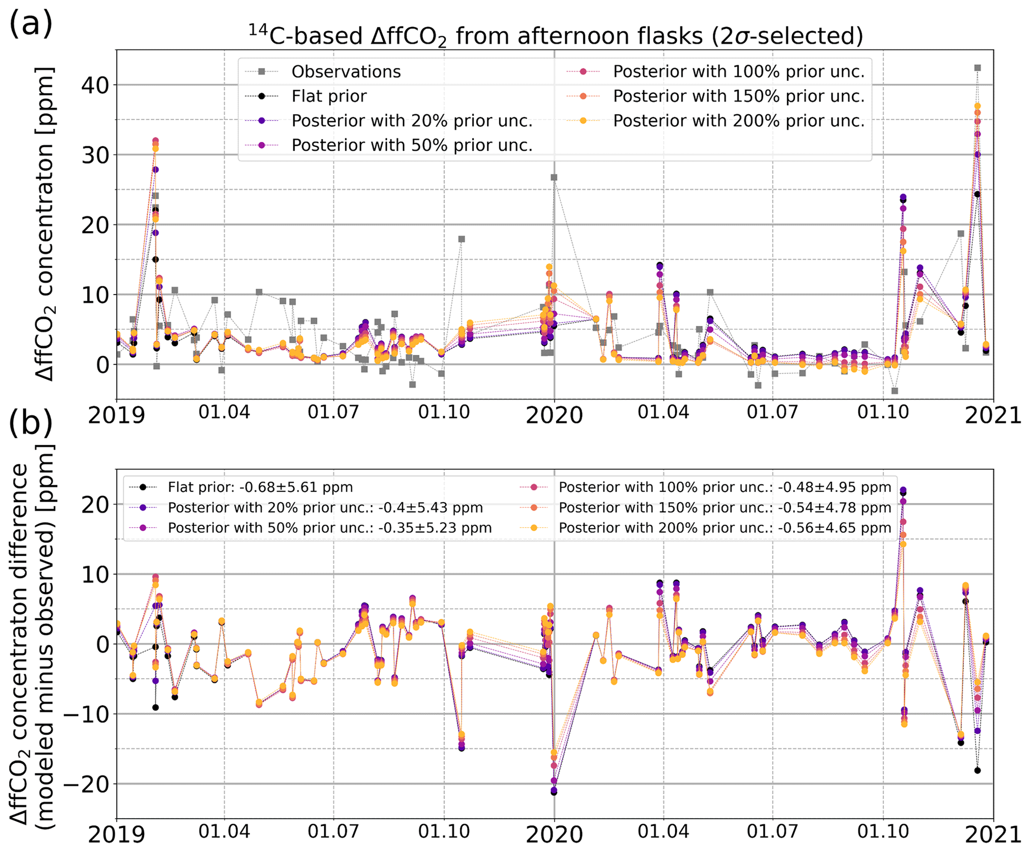
Figure B1 Comparison between the observed ¹⁴C-based ΔffCO₂ concentrations from the flasks and the modeled ΔffCO₂ concentrations based on the flat prior (black) and the different a posteriori emissions with prior uncertainties of between 20 % and 200 % (colored).

Appendix C: Impact of the averaging interval and additional degrees of freedom for the point sources emissions

To investigate the influence of inadequate point source modeling on the a posteriori area source ffCO₂ emissions, we use two different ΔCO-based ΔffCO₂ inversion setups: (1) an inversion with fixed point source emissions (“INV_fix”) and (2) an inversion with adjustable point source emissions (“INV_adj”). The first inversion setup corresponds to the inversion described in Sect. 2. It optimizes the flat a priori area source emissions by using fixed monthly point source emissions. The second inversion setup optimizes both the flat a priori area source emissions and the monthly a priori point source emissions. Thus, the point source emissions from the respective energy production sector and industry sector get the same temporal (i.e., “Filt3T” in CarboScope notation; see Sect. 2.2.6) and spatial (i.e., one spatial scaling factor) degrees of freedom as the area source emissions. Ideally, both inversion setups should lead to the same a posteriori area source emissions, meaning that the modeling of the better-known point source emissions has no influence on the area source emission estimates. Obviously, this is not the case. If the observed and modeled hourly ΔffCO₂ concentrations (i.e., the model–data mismatches) are not averaged over a certain period of time, the INV_fix inversion leads to much lower area source emissions estimates than the INV_adj inversion (see cyan curves in Fig. C1). For individual seasons, e.g., in summer 2020, the differences are larger than 150 %. Thus, the INV_fix inversion tends to decrease the area source emissions to compensate for an inadequate modeling of the (fixed) point source emissions. This indicates that the transport model (even with the VSI approach) and/or the TNO emission inventory seems to overestimate the contributions from point sources at the Heidelberg observation site for individual hours.

The averaging over one afternoon (magenta curve in Fig. C1) only leads to minor improvements; there are still deviations larger than 100 % in summer 2020. In contrast, the averaging interval of 1 week (blue curve) limits the largest deviations in summer 2020 to below 30 %. Averaged over the 2 years of 2019 and 2020, these deviations between the INV_fix and INV_adj a posteriori area source emissions are less than 10 %. A monthly averaging interval (pink curve) further reduces the deviations to below 20 % in summer 2020.

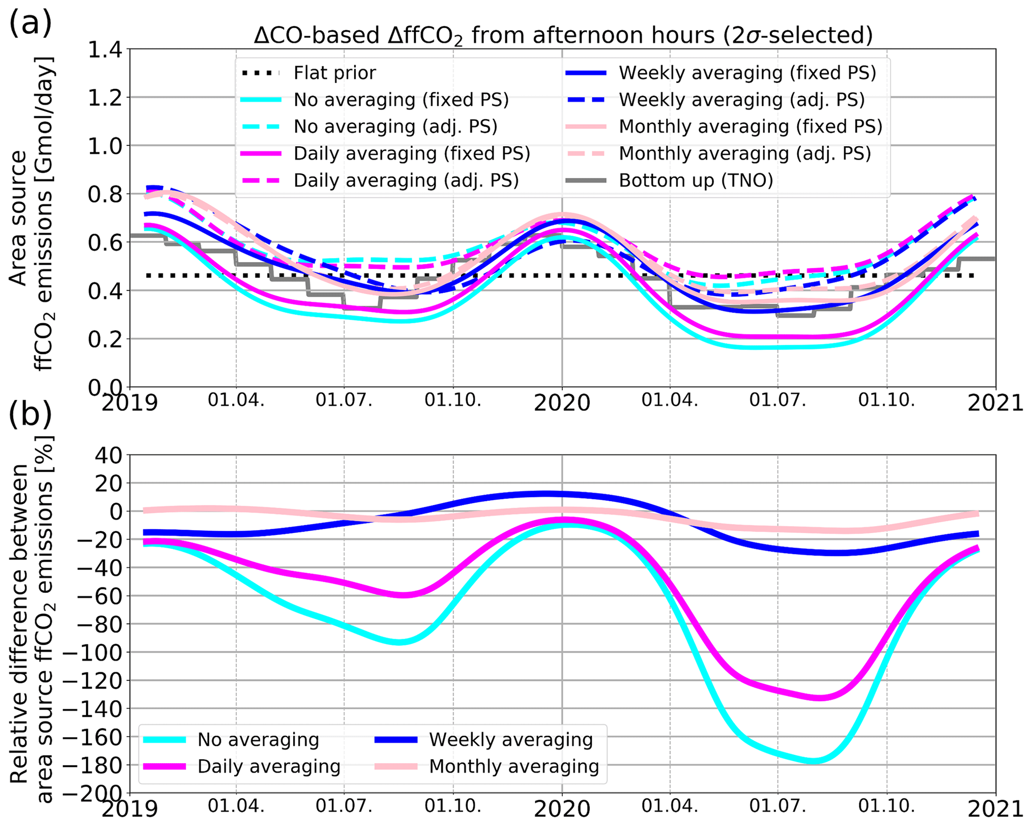
Figure C1 (a) Area source ffCO₂ emissions in the near field (blue outlined area in Fig. 1b) of Heidelberg. Shown are the results of the ΔCO-based ΔffCO₂ inversion with fixed point sources (solid lines, “fixed PS”) and adjustable point sources (dashed lines, “adj. PS”) for different averaging intervals ranging from no averaging at all (cyan) to daily averaging of the 5 h (11:00–16:00 UTC) of each afternoon (magenta) and weekly (blue) and monthly (pink) averaging. All a posteriori results correspond to a 150 % prior uncertainty. The flat a priori emissions and the bottom-up emissions are shown as a reference in black and gray, respectively. Panel (b) shows the relative differences (fixed PS minus adj. PS) between the a posteriori area source ffCO₂ emissions of the inversion runs with adjustable and fixed point source emissions (in %).

We also investigate if the sum of the a posteriori area source and point source emissions is similar for the INV_fix and the INV_adj inversion runs (see Fig. C2). If no averaging or only a daily averaging is applied, the INV_adj run leads to up to 50 % lower total (i.e., area plus point source) ffCO₂ emissions than the INV_fix run. This again shows that the point source emissions are strongly reduced in the INV_adj inversion run. A weekly averaging (blue curve) restricts the relative differences between INV_fix and INV_adj to below ca. 20 % if the first and the last 2 months of the 2-year period are disregarded. The monthly averaging again shows the smallest differences (below 10 %) between the INV_fix and the INV_adj run.

Figure C3 shows the comparison between the modeled ΔffCO₂ concentrations based on the INV_fix and INV_adj a posteriori emissions and the ΔCO-based ΔffCO₂ observations if a weekly averaging is applied (i.e., all hourly entries within 1 week are averaged in the model–data mismatch vector). The mean bias and the standard deviation between weekly averaged observed and modeled ΔffCO₂ are very similar for both inversion runs (0.10±1.89 ppm in the case of INV_fix and 0.13±1.80 ppm in the case of INV_adj). For comparison, the flat prior emissions lead to a mean bias of 0.65±2.23 ppm. Hence, there are no significant changes in the fits to the observational data when additional degrees of freedom are introduced for the point source emissions.

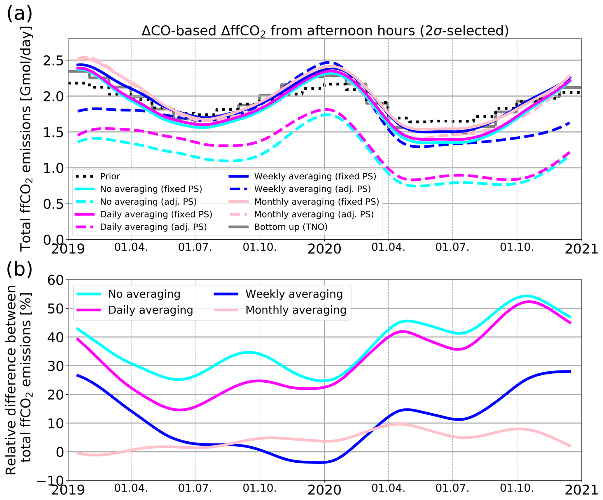
Figure C2 (a) Area plus point source (i.e., “total”) ffCO₂ emissions in the near field (blue outlined area in Fig. 1b) of Heidelberg. Shown are the results of the ΔCO-based ΔffCO₂ inversion with fixed point sources (solid lines, “fixed PS”) and adjustable point sources (dashed lines, “adj. PS”) for different averaging intervals ranging from no averaging at all (cyan) to daily averaging of the 5 h (11:00–16:00 UTC) of each afternoon (magenta) and weekly (blue) and monthly (pink) averaging. All a posteriori results correspond to a 150 % prior uncertainty. The a priori emissions and the bottom-up emissions are shown as a reference in black and gray, respectively. Panel (b) shows the relative differences (fixed PS minus adj. PS) between the a posteriori total ffCO₂ emissions of the inversion runs with adjustable and fixed point source emissions (in %).

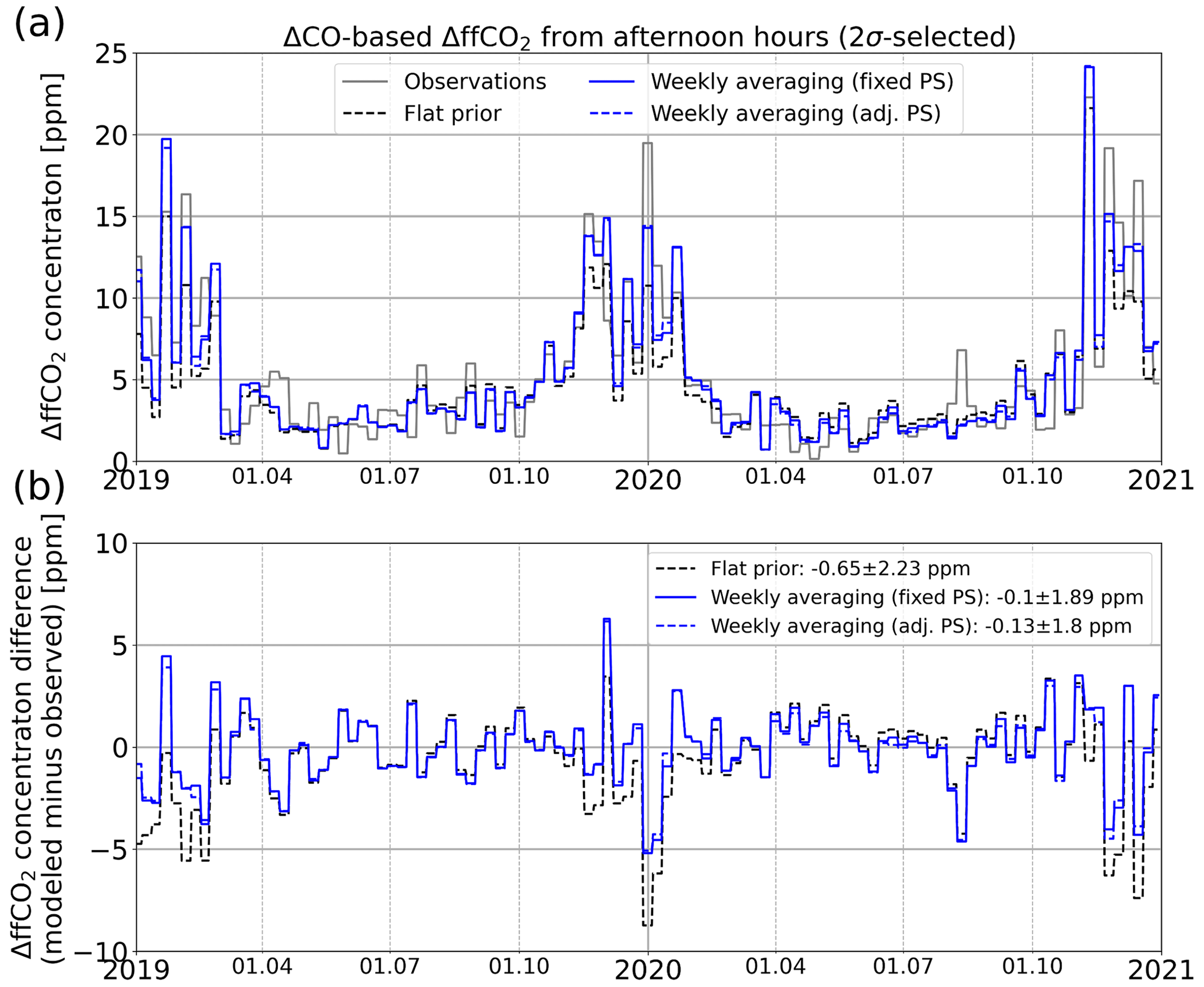
Figure C3 Comparison between the weekly averaged observed ΔCO-based ΔffCO₂ concentrations (gray) and the modeled ΔffCO₂ concentrations based on the flat prior (black) and the a posteriori emissions with a prior uncertainty of 150 % (blue). Shown are the results for the standard INV_fix inversion setup with fixed point source emissions (solid) and the INV_adj inversion setup with adjustable point source emissions (dashed). In both inversion setups, the hourly entries of the model–data mismatch vector within 1 week were averaged.

Appendix D: Anomaly in the seasonal cycle of the area source ffCO₂ emissions in 2020

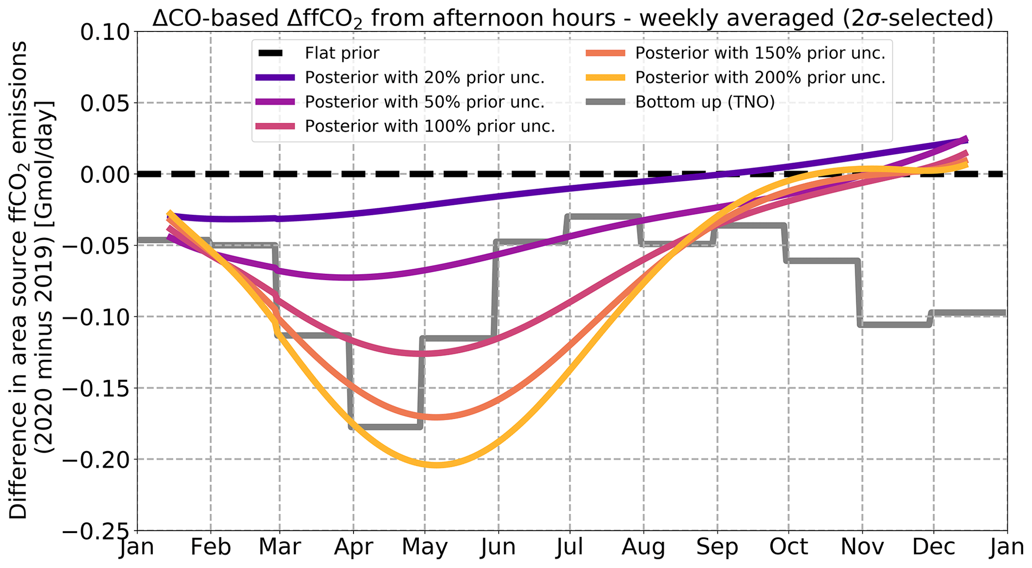
Figure D1 Difference in the near-field area source ffCO₂ emissions (in the blue outlined area in Fig. 1) between 2020 and 2019. Shown are the results of the ΔCO-based ΔffCO₂ inversion with fixed point sources and temporally flat prior emissions (see Fig. 4a).

Appendix E: Hypothetical seasonal cycle in the ΔCO$/\mathrm{\Delta }$ffCO₂ ratios

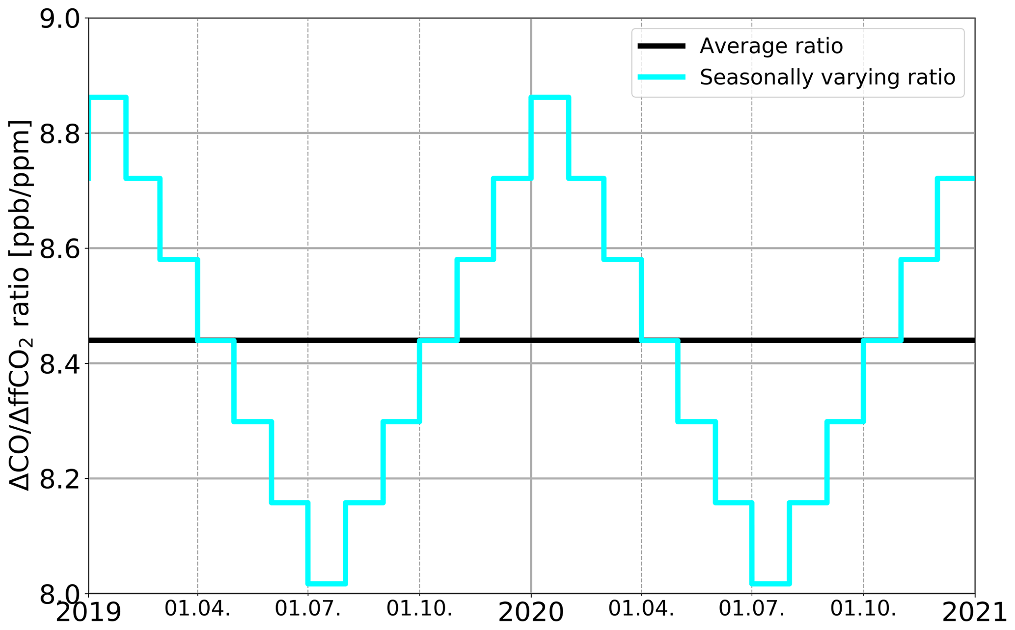
Figure E1 Average $\mathrm{\Delta }\mathrm{CO}/\mathrm{\Delta }{\mathrm{ffCO}}_{\mathrm{2}}$ ratio (black) and hypothetical seasonally varying ratio (cyan) used to construct the ΔCO-based ΔffCO₂ record for the base inversion (Fig. 4) and the sensitivity inversion run (cyan curve in Fig. 5), respectively.

Appendix F: Comparison between two modeled Rhine Valley ΔffCO₂ backgrounds

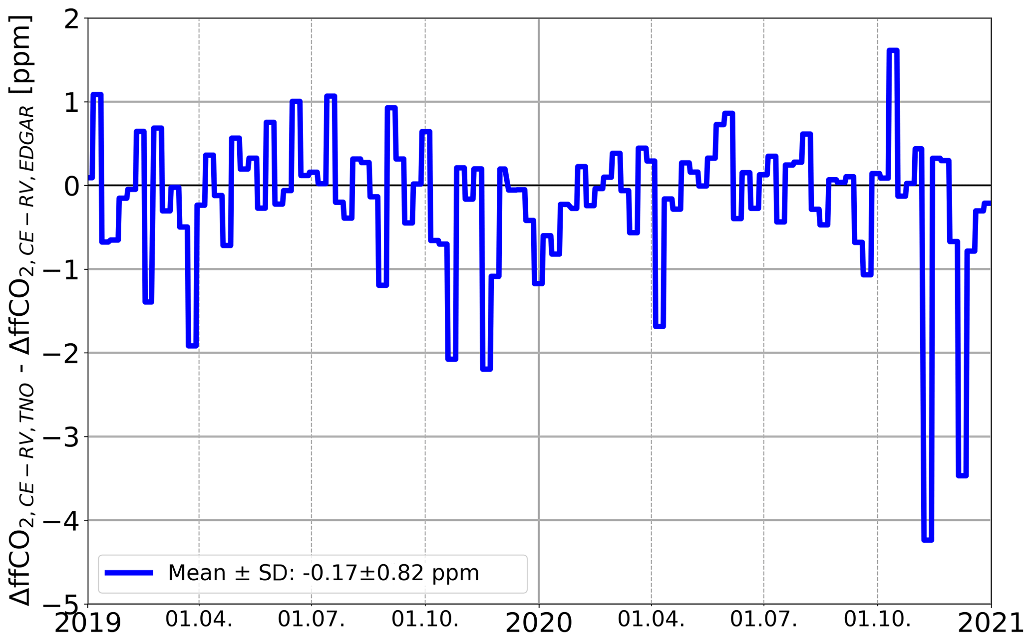
Figure F1 Difference between the Rhine Valley background modeled with TNO emissions (ΔffCO${}_{\mathrm{2},\mathrm{CE}\text{-}\mathrm{RV},\mathrm{TNO}}$) and the Rhine Valley background modeled with EDGAR emissions (ΔffCO${}_{\mathrm{2},\mathrm{CE}\text{-}\mathrm{RV},\mathrm{EDGAR}}$). Shown are weekly averages for afternoon situations.

Appendix G: Comparison between TNO and other emission inventories

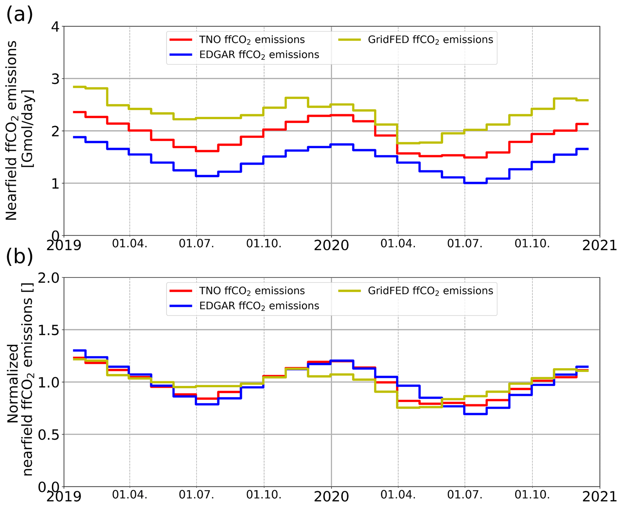
Figure G1 (a) Comparison between the TNO (red), EDGAR (blue), and GridFED (yellow) ffCO₂ emissions within the near-field area of Heidelberg (blue outlined area in Fig. 1b). Panel (b) shows the respective normalized near-field ffCO₂ emissions.