Exploring ozone variability in the upper troposphere and lower stratosphere using dynamical coordinates

Ozone trends in the upper troposphere and lower stratosphere (UTLS) remain highly uncertain because of sharp spatial gradients and high variability caused by competing transport, chemical, and mixing processes near the upper-tropospheric jets and extratropical tropopause as well as inhomogeneous spatially and temporally limited observations of the region. Subtropical jets and the tropopause act as transport barriers, delineating boundaries between atmospheric regimes controlled by different processes; they can thus be used to separate data taken in those different regimes for numerous purposes, including trend assessment. As part of the Observed Composition Trends And Variability in the UTLS (OCTAV-UTLS) Stratosphere-troposphere Processes And their Role in Climate (SPARC) activity, we assess the effectiveness of several coordinate systems in segregating air into different atmospheric regimes. To achieve this, a comprehensive dynamical dataset is used to reference every measurement from various observing systems to the locations of jets and tropopauses in different coordinates (e.g., altitude, pressure, potential temperature, latitude, and equivalent latitude). We assess which coordinate combinations are most useful for dividing the measurements into bins such that the data in each bin are affected by the same processes, thus minimizing the variability induced when combining measurements from different dynamical regimes, each characterized by different physical processes. Such bins will be particularly suitable for combining measurements with different sampling characteristics and for assessing trends and attributing them to changing atmospheric dynamics. Overall, the use of equivalent latitude and potential temperature leads to the most substantial reduction in binned variability across the UTLS. This coordinate pairing uses potential vorticity (PV) on isentropic surfaces, thus aligning with the adiabatic transport of tracers.

1 Introduction

The distribution of ozone in the upper troposphere and lower stratosphere (UTLS) region is crucial for Earth's radiation budget (e.g., Riese et al., 2012) and for modulating air quality near Earth's surface (e.g., Langford et al., 2015; Lin et al., 2015; Williams et al., 2019). Despite its importance and the decades of satellite, aircraft, balloon-borne, and ground-based measurements, confidence in the long-term ozone trends in the UTLS remains low (e.g., Harris et al., 2015; Steinbrecht et al., 2017; Petropavlovskikh et al., 2019; Szeląg et al., 2020; Godin-Beekmann et al., 2022). The difficulty in quantifying trends arises because the UTLS is a transition region between the ozone-poor troposphere and the ozone-rich stratosphere (Gettelman et al., 2011). UTLS ozone also exhibits high spatial and temporal variability driven primarily by variations in the UTLS jets and the tropopauses (e.g., Randel et al., 2007; Añel et al., 2008; Pan et al., 2009; Manney et al., 2011; Schwartz et al., 2015; Albers et al., 2018; Olsen et al., 2019). Measurements available in this region are spatially and temporally limited, resulting in inhomogeneous sampling of this variability. Moreover, the tropopause and the jets act as dynamical barriers to mixing, accompanied by strong changes in static stability (e.g., Birner, 2004) or strong isentropic potential vorticity (PV) gradients (e.g., Kunz et al., 2011a; Manney et al., 2011). Both lead to strong ozone and tracer gradients at the tropopause (Kunz et al., 2011b; Hegglin et al., 2008). Thus, tropopause (e.g., Pan et al., 2004; Hoor et al., 2004; Hegglin et al., 2009) or jet-relative (e.g., Manney et al., 2011; Olsen et al., 2019) coordinate systems have often been used to segregate air masses influenced by different dynamical processes (e.g., tropospheric versus stratospheric or poleward versus equatorward of the subtropical jet).

Another way of segregating air masses is by using coordinates that account for adiabatic conservation laws, i.e., PV–potential temperature (θ)-related coordinates. Rossby and smaller-scale waves lead to meridional displacements of air parcels that are mostly adiabatic and largely reversible in nature. PV–θ coordinates leverage the meridional distortions of PV contours as well as the movement of adiabatic parcels on surfaces of constant θ to account for these displacements (e.g., Hegglin et al., 2006). It is important to note that irreversible processes (diabatic processes such as radiative cooling or heating, turbulent mixing and stirring) modify PV on different timescales. These processes are associated with transport that leads to mixing and irreversible tracer exchange, likewise introducing ozone variability that cannot be accounted for by adiabatic coordinate transformations. Analyzing datasets in geometric coordinate systems (e.g., latitude–pressure grids) generally results in higher binned variability, as these coordinates do not account for the variability caused by changes in the positions of the jets or the tropopauses or for wave-induced air parcel displacements.

As part of the Observed Composition Trends And Variability in the UTLS (OCTAV-UTLS) Stratosphere-troposphere Processes And their Role in Climate (SPARC) activity, in this study we analyze how well different coordinate systems separate ozone measurements taken in atmospheric regimes dominated by different processes. Coordinate systems that effectively achieve this are expected to segregate observations into bins with reduced variability because measurements influenced by different (reversible) dynamical processes will not be averaged together. The datasets used include observations from the Aura Microwave Limb Sounder (MLS) and the Atmospheric Chemistry Experiment Fourier Transform Spectrometer (ACE-FTS) satellite instruments as well as high-resolution measurements from aircraft (including those from various research campaigns and the Civil Aircraft for the Regular Investigation of the atmosphere Based on an Instrument Container – CARIBIC-2), lidars, and ozonesondes.

Each data point from our observational datasets (see Sect. 2.1) comes with temporal and geolocation information. The geolocation information includes longitude and latitude in the horizontal and either altitude or pressure (or both) in the vertical. While these basic coordinates are essential for measurement retrievals and data processing, dynamically defined coordinates often facilitate interpretation of the data. Coordinate systems designed to show relationships with atmospheric phenomena are typically established with reference to the specific phenomenon itself, such as tropopause-relative coordinates. Conversely, dynamical coordinates such as potential temperature in the vertical or equivalent latitude (i.e., PV on isentropes) in the horizontal provide a framework (based on conservation laws for atmospheric motions) that aligns with the adiabatic movement of the air parcels.

Each of these coordinates remaps the data with respect to different aspects of dynamics, transport, or location. Thus, the coordinates that are most helpful for studying geophysical and transport properties of the data may be different for different regions and/or phenomena that are of interest. A key metric used to evaluate the impact of binning the data in each coordinate system is the binned variability. Depending on the coordinate system and its ability to account for tracer gradients at transport barriers between different air masses (e.g., at the tropopause or jet cores), the binning process can induce artificial variability on top of the inherent atmospheric variability (e.g., induced by nonconservative processes).

For example, Hegglin et al. (2008) discussed this enhanced variability when comparing datasets binned using tropopause-relative coordinates to those binned using altitude. This comparison revealed increased variability when the influence of the tropopause (and the tracer gradients associated with its location) was not accounted for, thereby highlighting the significance of dynamical variability. Since dynamical variability is an inherent property of the atmosphere, different representations of the data, i.e., coordinate systems that segregate dissimilar air masses, can minimize its effects on values grouped together in a bin, making it a useful metric for coordinate system comparison. We emphasize that neither the dynamical variability itself nor the atmospheric trace gas variability can be removed or minimized by any means – and indeed it is exactly this variability and the mechanisms for it that we ultimately want to isolate and study.

The choice of coordinate can, however, facilitate combination of measurements in each bin that are primarily affected by the same processes (thus reducing the variability in that bin) by accounting for transport history and/or the locations of transport barriers and thus strong tracer gradients. In other words, process-related coordinates can reduce binned variability, highlighting a more interpretable representation of the geophysical and trace gas variability and thus helping to elucidate the physical processes controlling it in different regions. The goal of this study is to show the effect of different coordinate systems on the binned variability. To achieve this, we use a variety of observational datasets together with reanalysis data.

Several abbreviations are used throughout this paper; all are defined the first time they appear in the text. However, to improve readability, a list of the abbreviations is provided in Appendix A (Table A1).

2 Datasets and binning methodology

2.1 Datasets

In this study, we use UTLS ozone observations from a diverse set of measurement techniques, in particular from ozonesonde, lidar, aircraft, and satellite datasets. These datasets have vastly different precision, accuracy, and temporal and spatial coverage. Table 1 provides a summary of the key characteristics of the different measurement systems, while Fig. 1 displays the sampling patterns. Further information for each dataset is presented below.

Sterling et al. (2018)Sterling et al. (2018)Stauffer et al. (2022)Sterling et al. (2018)Stauffer et al. (2022)Sterling et al. (2018)Stauffer et al. (2022)Sterling et al. (2018)Stauffer et al. (2020)Sterling et al. (2018)Stauffer et al. (2020)Sterling et al. (2018)Stauffer et al. (2020)Johnson et al. (2023)Steinbrecht et al. (2009)Ancellet et al. (1989)Pelon et al. (1986)McDermid et al. (2002)McDermid et al. (1990)McDermid et al. (1995)Bernet et al. (2020)Brenninkmeijer et al. (2007)Pan et al. (2010)Müller et al. (2016)Oelhaf et al. (2019)Waters et al. (2006)Bernath et al. (2005)

Table 1 Dataset characteristics.

^a For all the ozonesondes, the highest altitude depends on the bursting point of the balloon. ^b Electrochemical concentration. ^c Differential absorption lidar. ^d There are two different lidars at OHP, a stratospheric system (measuring since 1985) and a tropospheric one (measuring since 1991). ^e There are two different lidars at TMF, a stratospheric system (measuring since 1989) and a tropospheric one (measuring since 1999). ^f Typically between 10 and 13 km. ^g Photometry. ^h These campaigns all used the FAIRO instrument (Zahn et al., 2012). ⁱ Daily. ^j Seasonal.

Figure 1 Sampling patterns and locations of the ozone measurements used in this study. For the aircraft datasets (i.e., CARIBIC-2, TACTS/ESMVaL, PGS, and START08), we show all the sampling locations available during the 2005–2018 period. For the ozonesondes and lidar datasets, we display the site locations. For MLS and ACE-FTS we show representative daily and yearly sampling patterns, respectively.

2.1.1 Satellite remote instruments

Satellite instruments operate remotely, enabling them to provide global coverage. They differ in their observation geometry and in the wavelengths they may use to remotely sense the atmosphere, which influence the measurement characteristics, accuracy, precision, and sampling. In this study, we focus on two satellite limb sounders, Aura MLS and ACE-FTS, to exploit their long time series and maximize the overlap with other datasets.

Aura MLS

Aura MLS was launched aboard the Aura satellite in July 2004 (Waters et al., 1999, 2006). The spacecraft flies in a 98° inclined near-polar, sun-synchronous orbit, with a 13:45 local time ascending (north-going) Equator-crossing time at 705 km altitude that allows for observations from about 82° S to 82° N in each orbit. MLS uses heterodyne radiometers to observe thermal emission from the atmospheric limb in spectral regions centered near 118, 190, 240, and 640 GHz and 2.5 THz (i.e., at wavelengths of 2.54, 1.58, 1.25, 0.47, and 0.12 mm). From these radiances, temperature, trace gas concentrations, geopotential height, and cloud ice are retrieved. MLS provides about 3500 profiles (per species) along the suborbital track every day during both daytime and nighttime. The MLS ozone (Schwartz et al., 2020) vertical resolution in the UTLS is around ∼ 3 km.

ACE-FTS

ACE-FTS was launched aboard the SciSat-1 spacecraft in August 2003 (Bernath et al., 2005). The spacecraft has a drifting orbit at 650 km with an inclination of 74° that allows for observations from 85° S and 85° N. ACE-FTS profiles the atmosphere using a solar occultation technique, measuring one sunrise and one sunset per orbit, resulting in approximately 15 sunrise and 15 sunset occultations per day. Global coverage is achieved over a period of 3 months (i.e., one season), with almost exactly the same coverage year after year. ACE-FTS measures infrared spectra between 750 and 4400 cm⁻¹ at a high resolution (0.02 cm⁻¹) to derive volume mixing ratio profiles of over 50 atmospheric trace gas species and isotopologs (Boone et al., 2005). These measurements achieve an effective vertical resolution of around 1 km in the UTLS region due to vertical oversampling (Hegglin et al., 2008).

In comparison with MLS, ACE-FTS has a much lower sampling density and thus shows a seasonally varying sampling bias (Toohey et al., 2013; Millán et al., 2016; Hegglin and Tegtmeier, 2017). However, because of the very high signal-to-noise ratio of the solar occultation technique, ACE-FTS measurements are typically more precise than those from MLS.

2.1.2 Airborne in situ instruments

Aircraft in situ measurements for this study were typically made using chemiluminescence detectors and/or UV photometry. In this study we use data from four campaigns:

• Stratosphere-Troposphere Analyses of Regional Transport 2008 (START08; Pan et al., 2010);

• Transport and Composition in the Upper Troposphere and Lower Stratosphere and Earth System Model Validation (TACTS/ESMVal; Müller et al., 2016);

• the Polar Stratosphere in a Changing Climate (POLSTRACC; Oelhaf et al., 2019) campaign, operated with two other projects, the Investigation of the Life cycle of gravity waves (GW-LCYCLE) and Seasonality of Air mass transport and origin in the Lowermost Stratosphere (SALSA), known collectively as the PGS mission; and

• the In-service Aircraft for a Global Observing System (IAGOS; Petzold et al., 2015; Thouret et al., 2022) and CARIBIC (Brenninkmeijer et al., 1999, 2007).

Typical random errors for the ozone measurements in these campaigns are smaller than 1 % (e.g., Zahn et al., 2012). In comparison to satellite instruments, in situ measurements on aircraft generally have limited temporal and spatial coverage globally, as shown in Fig. 1. However, CARIBIC-2 aircraft operate at cruising altitudes of 10–13 km, near the climatological location of the extratropical tropopause. The high temporal and horizontal sampling of CARIBIC-2 provides a very detailed view of the tropopause and a very long time series (starting in 1997). In contrast, the other aircraft missions studied here, START08, PGS, and TACTS/ESMVal, have more limited regional and temporal coverage but provide more extensive vertical coverage of the UTLS, making them ideal for process-oriented studies. Thus the set of all aircraft datasets used here provides complementary views of the UTLS.

2.1.3 Lidars

This study uses data from several ground-based ozone differential absorption lidars (DIALs; Mégie et al. (1977)). Different wavelengths are used for tropospheric (Hartley band: 266–300 nm) and stratospheric ozone (Higgins band: 300–360 nm) to ensure adequate sensitivity to the drastically different ozone concentrations in the two regions. Stratospheric lidar measurements used here are taken at Table Mountain, Mauna Loa, Haute-Provence, Hohenpeissenberg, and Lauder; tropospheric lidar measurements are from Table Mountain and Haute-Provence (see Fig. 1).

Because of the wavelength dependence, stratospheric ozone lidars only operate at night, while tropospheric ozone lidars operate at any time of the day (with a limited signal-to-noise ratio during daytime). In this study, only nighttime data are used to keep consistency between the tropospheric and stratospheric lidar datasets. Instruments operate for any duration from a few minutes to several days (sometimes weeks) without interruption, typically recording one to five profiles a week at 5 %–20 % relative uncertainty in the UTLS. Most lidars achieve a high vertical resolution on the order of less than 1 km. Temporal and vertical resolution can be tuned to achieve specific uncertainty requirements (Leblanc et al., 2016a, b). The characteristics of the lidars used in this study are given in Table 1.

In comparison with satellite instruments, lidars can capture the temporal evolution of vertical ozone profiles over a given location with a relatively high vertical resolution and accuracy, but the geographical coverage is limited by the actual number of instrument locations.

2.1.4 Ozonesondes

The ozonesonde profiles used in this study (see Table 1 for details) are from balloons launched at eight stations (Summit, Greenland; Trinidad Head, USA; Boulder, USA; Hunstville, USA; Hilo, USA; PagoPago, American Samoa; Suva, Fiji; Amundsen-Scott South Pole, Antarctica). The Boulder, Hilo, and Trinidad Head stations have weekly ozonesonde launches, while American Samoa and Fiji launch ozonesondes only twice a month, with occasional gaps in the time series. The sampling at the South Pole station is typically weekly to biweekly, except during the ozone depletion season (September–October), when sampling can be as frequent as every other day to map the rate of the ozone decline in the lower stratosphere (Johnson et al., 2023). Since around 2001 (depending on the station), the data have been collected with 1 Hz frequency, yielding a vertical resolution between 5 and 300 m.

In this study, ozonesondes were gridded to 100 m to reduce computing power when calculating the dynamical diagnostics (see Sect. 2.2). It is important to note that this gridding resolution has no impact on the study's results, as the reanalysis fields only contain information at about 1 km vertical spacing and measurements will be averaged together in approximately 1 km bins. Lower-stratospheric uncertainties of ozonesondes are about ± 4 %–6 %, while in the upper troposphere they are around ± 5 % in the tropics and around ± 20 % at the mid latitudes (e.g., Smit et al., 2007; Sterling et al., 2018; Tarasick et al., 2021; Smit and Thompson, 2021). The ozonesonde records have been homogenized to remove instrumental steps (Sterling et al., 2018).

Note that Stauffer et al. (2020) identified an instrument artifact that has caused total column ozone measurements from some stations to drop by 3 %–7 %, including Hilo, Fiji, and American Samoa. Subsequently, Stauffer et al. (2022) found that these drop-offs may be related to changes in the pump efficiency. These drop-offs were typically limited to pressures above ∼ 50 hPa, which is approximately the upper limit of the vertical range used in this study. Therefore, the results shown here should generally be unaffected.

In comparison with satellite instruments, ozonesondes, similarly to lidars, can capture the temporal evolution of vertical ozone profiles over a given location with high vertical resolution and accuracy, albeit with spatial coverage limited by the number of launch stations.

The datasets used in this study are not intended to be comprehensive; numerous other ozone records are available, e.g., limb scattering satellite sounders, such as the Optical Spectrograph and Infrared Imager System (OSIRIS; Llewellyn et al., 2004) or the Ozone Mapping and Profiler Suite (OMPS; Seftor et al., 2014), the long-term airborne measurements from IAGOS-CORE (Petzold et al., 2015), and the ozonesondes included in the Southern Hemisphere ADditional OZonesondes (SHADOZ; Witte et al., 2017; Thompson et al., 2017). However, the records included are representative of the currently available measurement techniques in terms of resolution and geophysical sampling of the UTLS.

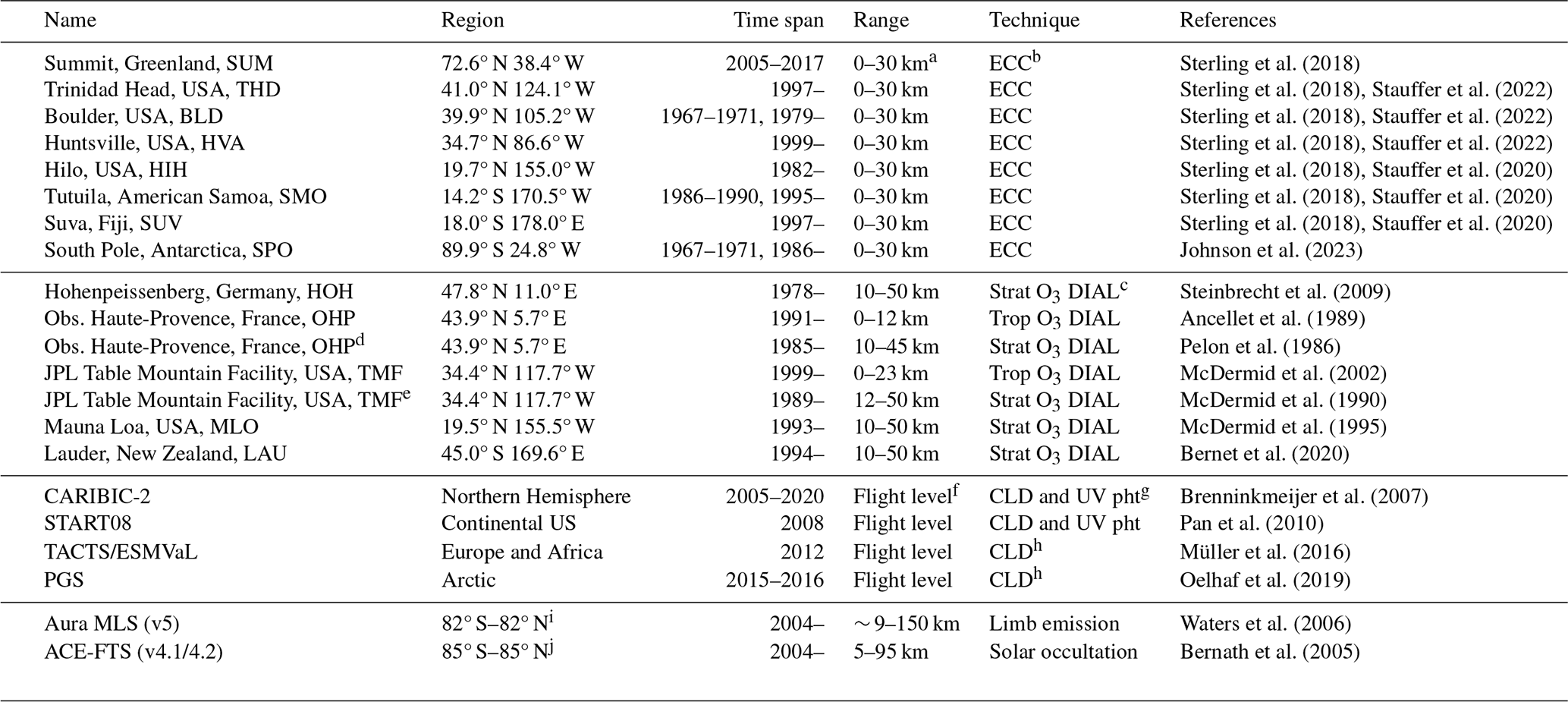
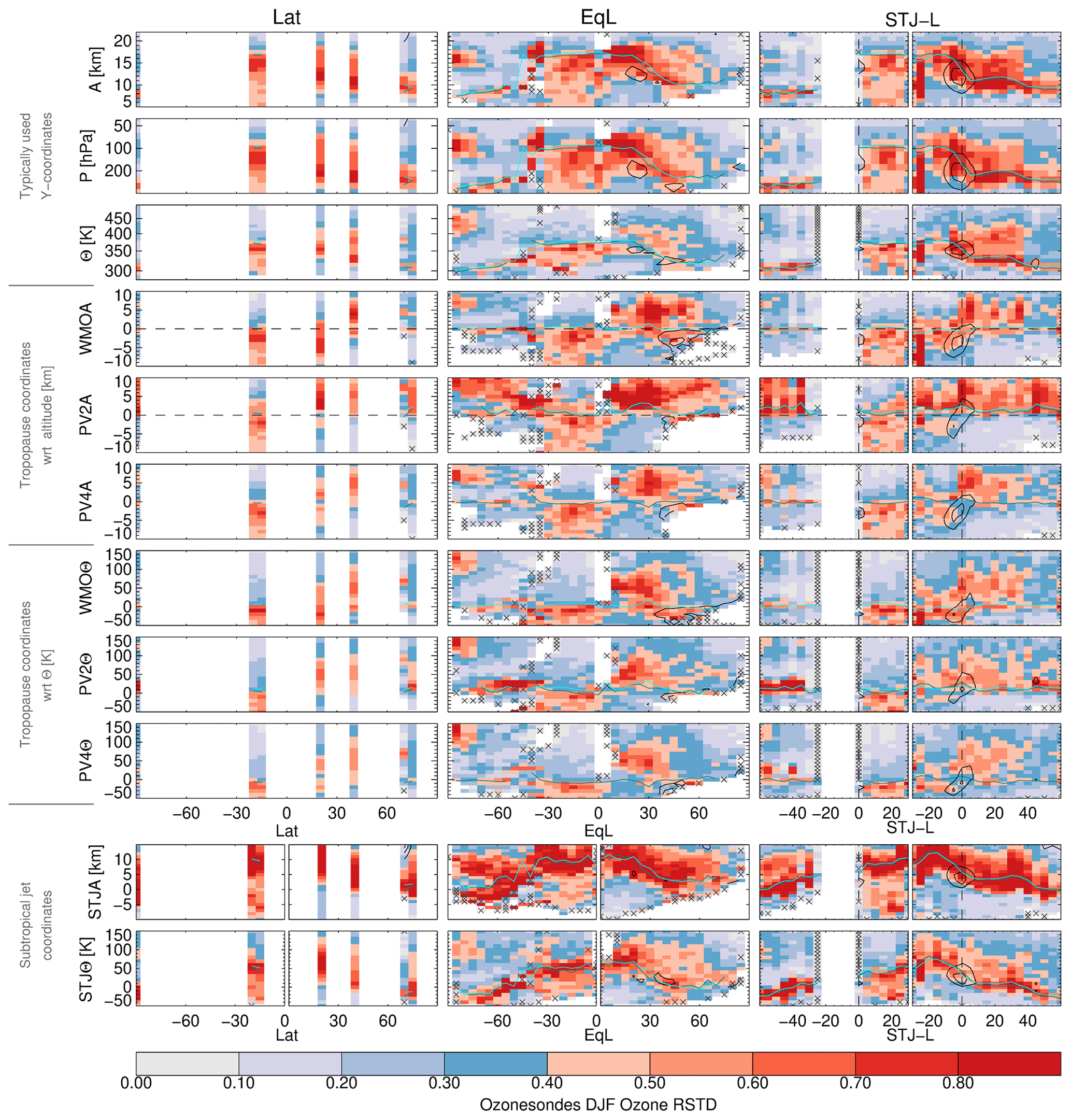
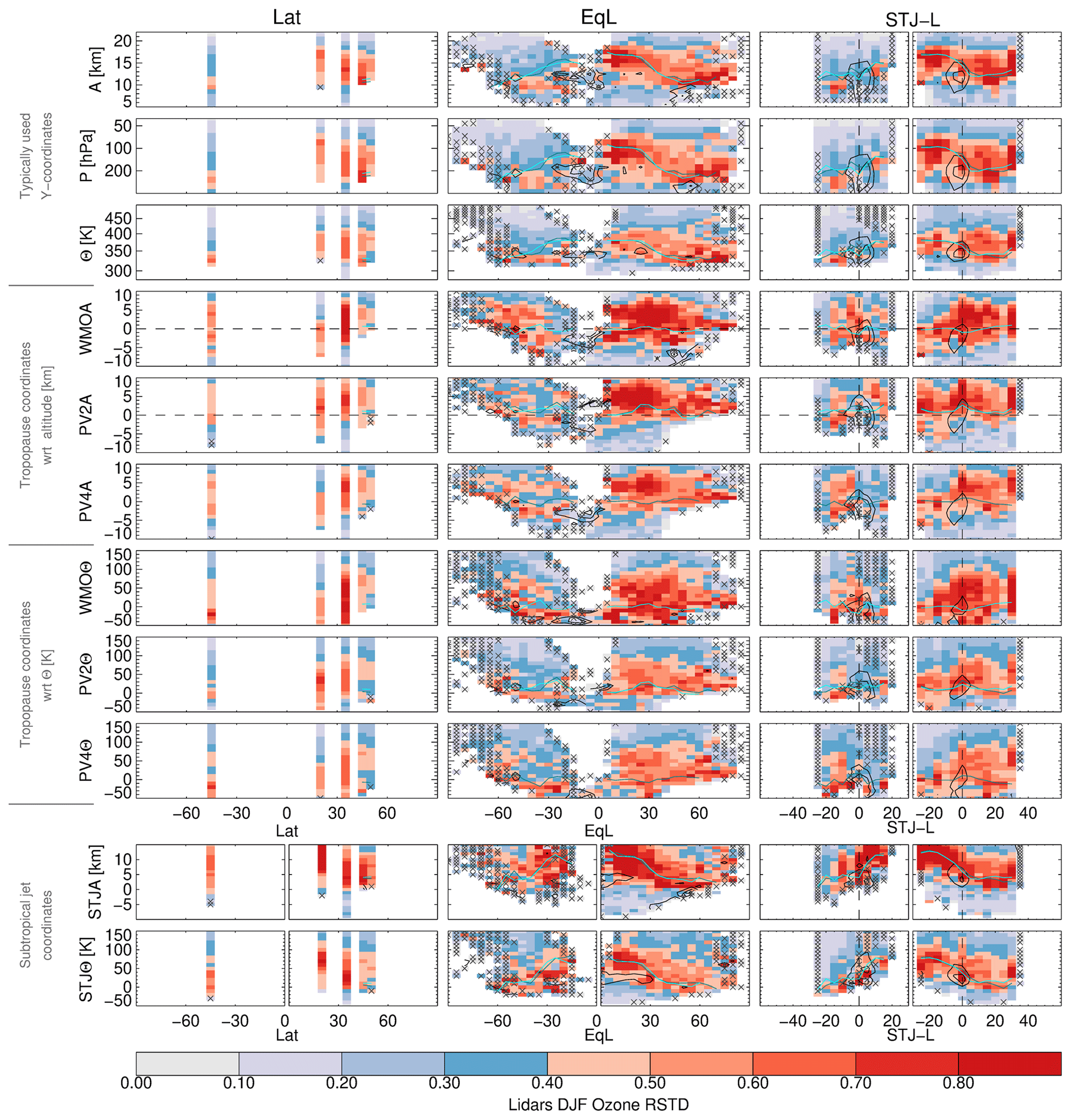
Figure 2 DJF (2005–2018) mean ozone distributions for MLS, ACE-FTS, aircraft, ozonesondes, and lidars as a function of latitude and altitude, pressure, or potential temperature. Cyan lines show the 4.5 PVU dynamical tropopause and teal lines the WMO (thermal) tropopause. The black contours show wind speed values of 30, 40, and 50 ms⁻¹. Note that differences in the wind representation in comparison with MLS suggest sampling biases. Crosses indicate bins where there are fewer than 10 measurements.

2.2 Method

2.2.1 Jet and tropopause characterization

To conduct a comprehensive analysis of the effects different coordinate systems can have on the variability of these ozone datasets, supplementary information regarding the atmospheric dynamical conditions that affect them is essential. In the context of the transport-relevant coordinates sought here, the information used in this study is potential temperature, equivalent latitude (the latitude that would enclose the same area between it and the pole as each isentropic potential vorticity contour), subtropical jet locations (derived from wind speeds), and the tropopause locations at each measurement time and location. These dynamical fields were computed using the JEt and Tropopause Products for Analysis and Characterization (JETPAC) algorithms, which are described in detail by Manney et al. (2011), Manney et al. (2014), Manney et al. (2017), Manney et al. (2021b), and Manney and Hegglin (2018). A complete overview of the latest JETPAC configuration used here is given by Millán et al. (2023).

In short, JETPAC provides potential temperature, equivalent latitude, and dynamical (PV-based) and World Meteorological Organization (WMO, temperature gradient) tropopause locations and conditions as well as the locations and dynamical characteristics of the UTLS jets for each of the measurement locations of the disparate datasets used here. JETPAC computes these fields from reanalysis datasets, in this case the Modern-Era Retrospective analysis for Research and Applications, version 2 (MERRA-2; Gelaro et al., 2017). MERRA-2 provides meteorological fields at 3 h intervals, on a 0.625°–0.5° latitude–longitude grid with 72 hybrid σ-pressure levels between the surface and 0.01 hPa. The UTLS vertical spacing is about 1.2 km. MERRA-2 products have been extensively evaluated and found to be well-suited for UTLS studies (Manney et al., 2017, 2021a, c; Manney and Hegglin, 2018; Xian and Homeyer, 2019; Homeyer et al., 2021; Fujiwara et al., 2022; Tegtmeier et al., 2022).

By using the same algorithms and the same reanalysis fields for all the datasets, we ensure that the derived dynamical conditions are consistent throughout the diverse datasets used in this study. This consistency facilitates the examination of these datasets with varying sampling characteristics, uncertainties, and resolutions in a unified dynamical framework. This framework allows us to explore the impact of different dynamical coordinate systems such as equivalent latitude, potential temperature, the tropopause, and jet-relative coordinates as well as to compare them with conventional coordinates such as latitude, altitude, and pressure.

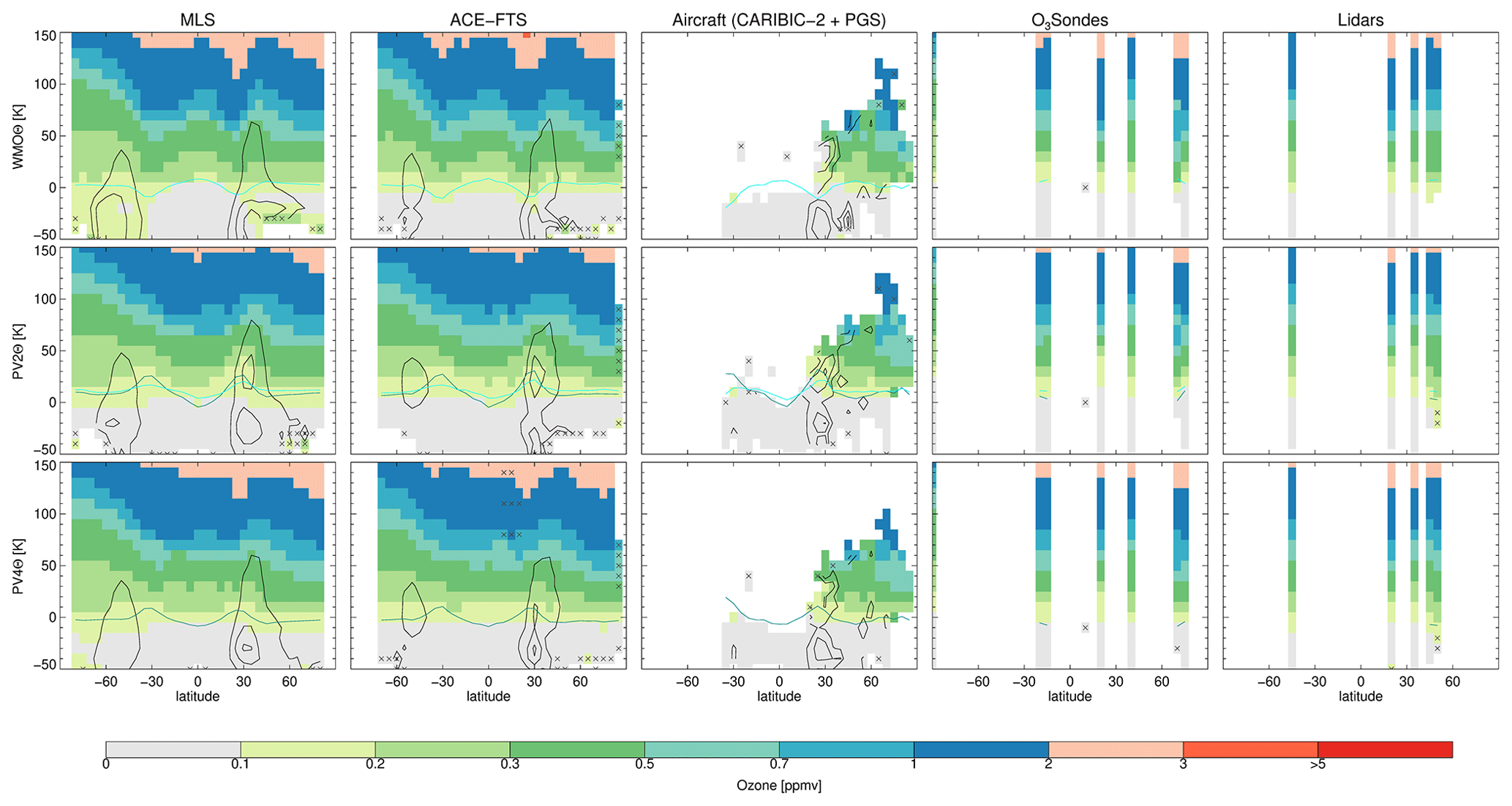
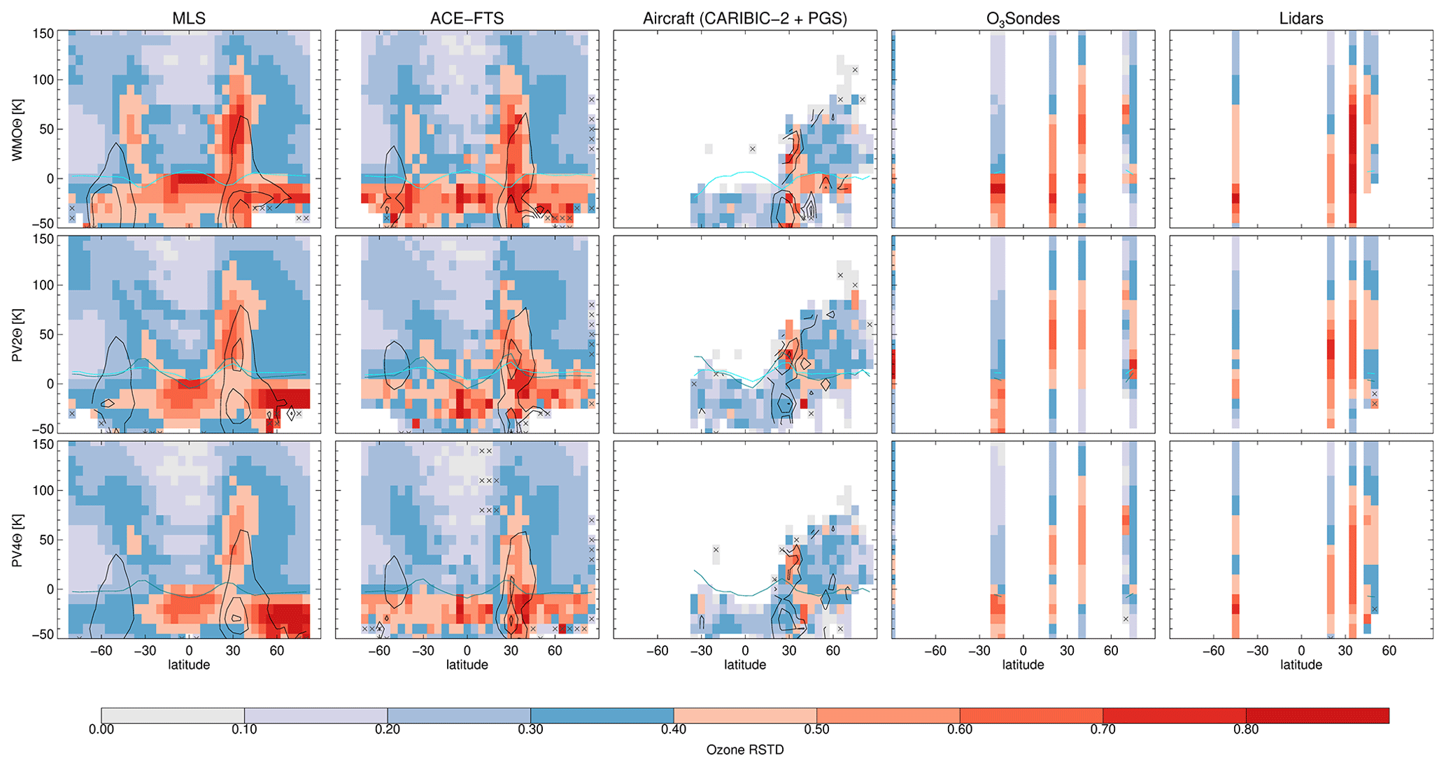
Figure 3 As in Fig. 2, but the vertical coordinates represent a potential temperature difference with respect to the tropopause defined by the WMO criteria: 2 PVU or 4.5 PVU threshold.

Figure 4 As in Fig. 2, but the vertical coordinate is potential temperature and the horizontal coordinates in the three rows are latitude, equivalent latitude, and distance in latitude from the STJ (i.e., STJ-L).

2.2.2 Coordinate mapping

We examine the effects of different coordinate systems on the representation of geophysical variability in UTLS ozone through production of climatologies from the datasets outlined in Sect. 2.1. For this initial study, we use averages over all longitudes with different horizontal coordinates, similar to zonal means when using latitude. However, many dynamical and chemical processes exhibit significant longitudinal variations. Consequently, as mentioned in the Introduction, coordinates that are most helpful for studying geophysical and transport properties may vary depending on the region or phenomenon of interest.

Because the variability in climatologies used here is also influenced by sampling and measurement characteristics, the use of multiple datasets allows exploration of the commonalities among differences in climatologies as a function of the coordinate system for each instrument. Any common changes between coordinate systems are assumed to result from a change in the representation of the effects of geophysical variability.

In this study, we focus on 3-month climatological periods, using data spanning 2005 through 2018. We choose this period due to the current availability of dynamical diagnostics (discussed in the previous Sect. 2.2.1), which require significant computing time to generate. This period allows for ample overlap among all the measurement techniques used here, i.e., ozonesondes, lidars, aircraft in situ campaigns, and limb sounders. While the aircraft in situ measurements from PGS, TACTS/ESMVaL, and START08 do not cover the entire period, we include them to enhance the coverage of this measurement technique. However, it is worth noting that the bulk of the variability, in the aircraft results, is driven by the overwhelming quantity of CARIBIC-2 measurements.

In particular, we focus on December–January–February (DJF) climatologies constructed for this 14-year period to investigate the perspective given by using different coordinate systems. Results for the June–July–August (JJA) period are provided in the Appendix for further reference. We highlight these seasons to focus on the periods where the subtropical jet is predominant in the Northern Hemisphere (DJF) as well as in the Southern Hemisphere (JJA) (e.g., Spensberger and Spengler, 2020; Manney et al., 2014). Results for March–April–May (MAM) and September–October–November (SON) were analyzed but are not shown.

All information on the dynamical coordinates (e.g., equivalent latitude, jet and tropopause characteristics) used in the construction of the climatologies is calculated using JETPAC. In the vertical, data are binned from their native pressure or altitude onto uniform vertical grids using either altitude, pressure, or potential temperature, with the bounds of each chosen to span approximately the same vertical range within the UTLS. Figure 2 illustrates the redistribution of ozone across these three coordinates when plotted versus latitude as the horizontal coordinate. While the ozone distributions share some broad similarities, notable differences are observed, showcasing the impacts of using different vertical coordinates. The impact of these coordinates on the ozone variability will be discussed in Sect. 3.

Figure 5 As in Fig. 2 but displaying the ozone relative standard deviation.

Figure 6 As in Fig. 3 but displaying the ozone relative standard deviation.

Additional vertical coordinates are constructed by setting the altitude or potential temperature in reference to the tropopause or the subtropical jet (STJ) core. In this study, three tropopause definitions were considered: the WMO-defined lapse rate tropopause, the dynamically defined 2 potential vorticity unit (PVU), and the 4.5 PVU tropopause. In total, this results in 11 vertical grids, as outlined in Table 2. An example of these relative coordinates is illustrated in Fig. 3, which shows ozone plotted as a function of latitude and potential temperature relative to the three tropopauses used in this study. Tropopause coordinates segregate measurements taken in the troposphere from those taken in the stratosphere, leading to strong gradients at the zero coordinate level (i.e., the tropopause). The usefulness of these coordinates in minimizing binned variability depends on how well the corresponding tropopause captures these ozone gradients as well as the vertical resolution of the measurements in question. The bounds of the vertical coordinate grids were chosen to minimize contributions from the lower troposphere and middle stratosphere to the UTLS climatologies.

Table 2 Vertical coordinate grids employed in this study, along with their vertical ranges and resolution.

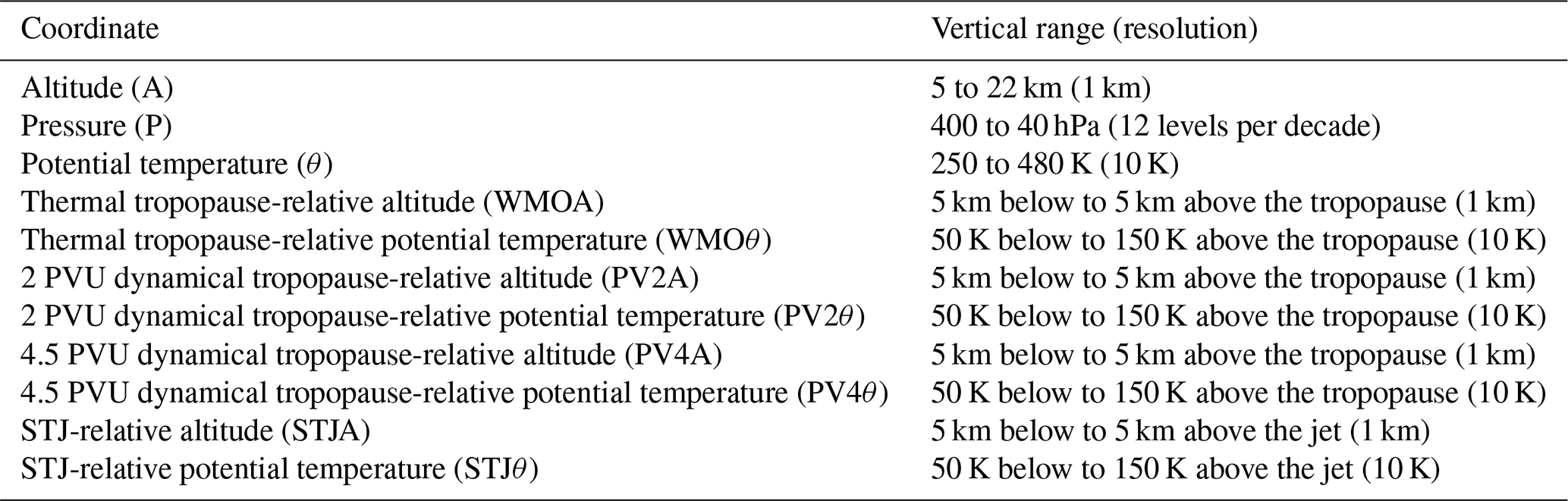
In the horizontal, data are binned onto grids using either geographic latitude, equivalent latitude, or STJ-relative latitude (STJ-L). Each of these coordinates uses a 5° spacing, but the geographic and equivalent-latitude grids span 90° N to 90° S, while the STJ-L grid spans 30° equatorward to 60° poleward of the jet core. The influence of the jets is limited to a smaller latitudinal range than what is employed here. However, the 30°–60° range allows us to compare against other coordinate systems in the most straightforward manner. These horizontal coordinates are summarized in Table 3 and illustrated in Fig. 4 using potential temperature as the vertical coordinate. Note that, when referring to the STJ-L, we divide the data into hemispheres resulting in the two subpanels per dataset as shown in the bottom row of Fig. 4. This separation by hemisphere is also performed when referring to the subtropical jet core in the vertical.

The effect of the dynamical remapping using equivalent-latitude or jet-based coordinates is most noticeable for the ozonesonde and lidar datasets. These observations are made near fixed geographical latitudes but for different dynamical conditions (e.g., south of the STJ or north of the STJ, different tropopause altitudes). The use of dynamical coordinates bins the data according to dynamical regimes, thus accounting for the dynamical conditions over time at a fixed location. It therefore expands their “condition-space” coverage to span much of the globe.

Table 3 Horizontal coordinate grids employed in this study, along with their ranges and resolution.

For each coordinate bin (spanning 5° in the horizontal coordinate and the vertical spacing outlined in Table 2), we quantified the variability using the relative standard deviation, RSTD, given by

$$\begin{array}{}\text{(1)}& \mathrm{RSTD}={\displaystyle \frac{\mathit{\sigma }}{\stackrel{\mathrm{‾}}{x}}},\end{array}$$

where $\stackrel{\mathrm{‾}}{x}$ is the mean volume mixing ratio, and σ is the standard deviation of the bin. The RSTD is used to evaluate the variability of the climatologies, as it provides a measure of spatial variance that is scaled and thus independent of the magnitude of the mean concentration within each coordinate bin, enabling effective comparisons across the UTLS.

3 Results

Before conducting a comparison involving all 33 coordinate systems, we assess the RSTD and the underlying properties for the coordinate systems illustrated in Fig. 2 through Fig. 4. The RSTD equivalents of those figures are shown in Fig. 5 through Fig. 7. It is important to note that the aircraft, ozonesonde, and lidar datasets have much sparser coverage, particularly for the latter two, in latitude-based coordinates than ACE-FTS and MLS. Additionally, ACE-FTS and lidar observations are limited to clear-sky conditions due to their inability to penetrate most clouds. MLS has the coarsest vertical resolution, causing smearing of both observations and the variance (Livesey et al., 2020). The aircraft measurements are mostly limited to flight levels but allow for the detection of more variability in the measurement region due to the high temporal sampling. By examining these diverse datasets, the impacts of each individual limitation in resolution or sampling can be assessed and ozone variability characteristics that are robust across all the datasets can be identified. As a reference, Fig. B1 showcases the number of measurements per bin available for each observation system and for several coordinate systems used in this study.

Figure 5 shows the influence on the relative standard deviation of using different traditional vertical coordinates versus latitude. The tropopause region can be clearly identified as a region of high ozone variability in all five datasets. In altitude and pressure coordinates, the variability associated with this feature extends well into the troposphere, particularly for MLS as a consequence of its coarser vertical resolution. However, when employing potential temperature, which effectively captures rapid quasi-isentropic transport and accounts for vertical displacements of the adiabats in altitude or pressure coordinates, a decrease in the vertical extent of this high binned variability (high RSTD values) becomes apparent. This effect is particularly evident in the MLS, ACE-FTS, and aircraft datasets but can be inferred from the ozonesonde and lidar plots as well. Thus the potential temperature vertical coordinate helps account for some of the geophysical variability seen when binning the data at altitude or pressure.

Moreover, MLS and ACE-FTS display particularly high RSTD values around the northern STJ, which constitutes a stronger transport barrier in DJF compared to summer. Specifically, the STJ separates tropical and midlatitude air, leading to intense ozone gradients near the jet location. Variability in this region manifests itself as high RSTD values resulting from variations in the latitude of large ozone gradients. In altitude and pressure coordinates, the jet-associated variability mostly falls along the tropopause. However, when employing potential temperature, the jet-induced variability manifests itself more prominently as a distinct lobe of variability located mostly above the STJ. Overall, as a function of latitude, potential temperature not only reduces the overall binned variability, but also clarifies the structure of the two main sources of variability (i.e., tropopause and STJ variations), which cannot be separated when using altitude or pressure coordinates.

When changing the vertical coordinate to potential temperature relative to the tropopause(s), as shown in Fig. 6, it is apparent that the effect of remapping to tropopause-referenced coordinates tends to agglomerate the variability in the bins along the transport barriers, i.e., where gradients are strong enough to make for substantial changes within one bin. MLS and ACE-FTS display high RSTD lobes around 30° S and 30° N (also hinted at by the lidars), which correspond to the regions where double tropopauses (e.g., Randel et al., 2007; Añel et al., 2008; Schwartz et al., 2015; Olsen et al., 2019) associated with tropospheric and stratospheric intrusions are preferentially found. In these regions, the choice of one reference surface leads to high variability in a fixed latitude framework. The location of the double tropopauses varies with latitude, longitude, and time. The binning process then mixes measurements within latitude bins where vertical profiles are taken relative to the lower (primary) and upper (secondary) tropopause at different longitudes, resulting in the large RSTD at the jet location high into the lower stratosphere. Moreover, in between the primary and secondary tropopause, only accounting for the vertical distance relative to the tropopause fails to account for the presence of air masses of tropospheric and stratospheric origin that are quasi-horizontally (i.e., quasi-isentropically) advected between these levels (e.g., Pan et al., 2009; Wang and Polvani, 2011; Schwartz et al., 2015), leading to high RSTD values.

By intercomparing the panels in Fig. 6, it is evident that the RSTDs are overall smaller when binning with respect to either the 2 PVU (PV2θ) or 4.5 PVU dynamical tropopause (PV4θ) than when binning with respect to the WMO tropopause (WMOθ). In particular, this is noticeable in the lobes of high RSTDs around 30° S and 30° N seen in MLS and ACE-FTS and hinted at in the ozonesonde and lidar panels. Further, the RSTD also displays smaller values for the aircraft datasets in the extratropics, with the PV4θ coordinate generally accounting for variability better than the PV2θ coordinate. This is because the 2 PVU surface better represents the tropopause at the middle and high latitudes (Hoor et al., 2004; Kunz et al., 2015), while higher PV values best represent the tropopause for the subtropics (Kunz et al., 2015; Berthet et al., 2007). In general, Fig. 6 suggests that dynamical tropopause-based coordinates resolve the ozone gradients across the tropopause region better than the WMO tropopause-based coordinate. This is not unexpected as the WMO tropopause results in breaks and multiple tropopauses between the tropics and the extratropics (e.g., Randel et al., 2007; Pan et al., 2009; Homeyer et al., 2010) rather than a continuous transition as provided by the dynamical (PV) tropopauses. Compared to other datasets, MLS displays larger RSTD values in the northern extratropics and smaller values in the southern extratropics in the tropopause-based coordinates. Despite its coarse vertical resolution potentially failing to properly resolve the tropopause, this RSTD value might be related to its better coverage of the region; i.e., MLS might sample more variability.

Figure 7 As in Fig. 4 but displaying the ozone relative standard deviation.

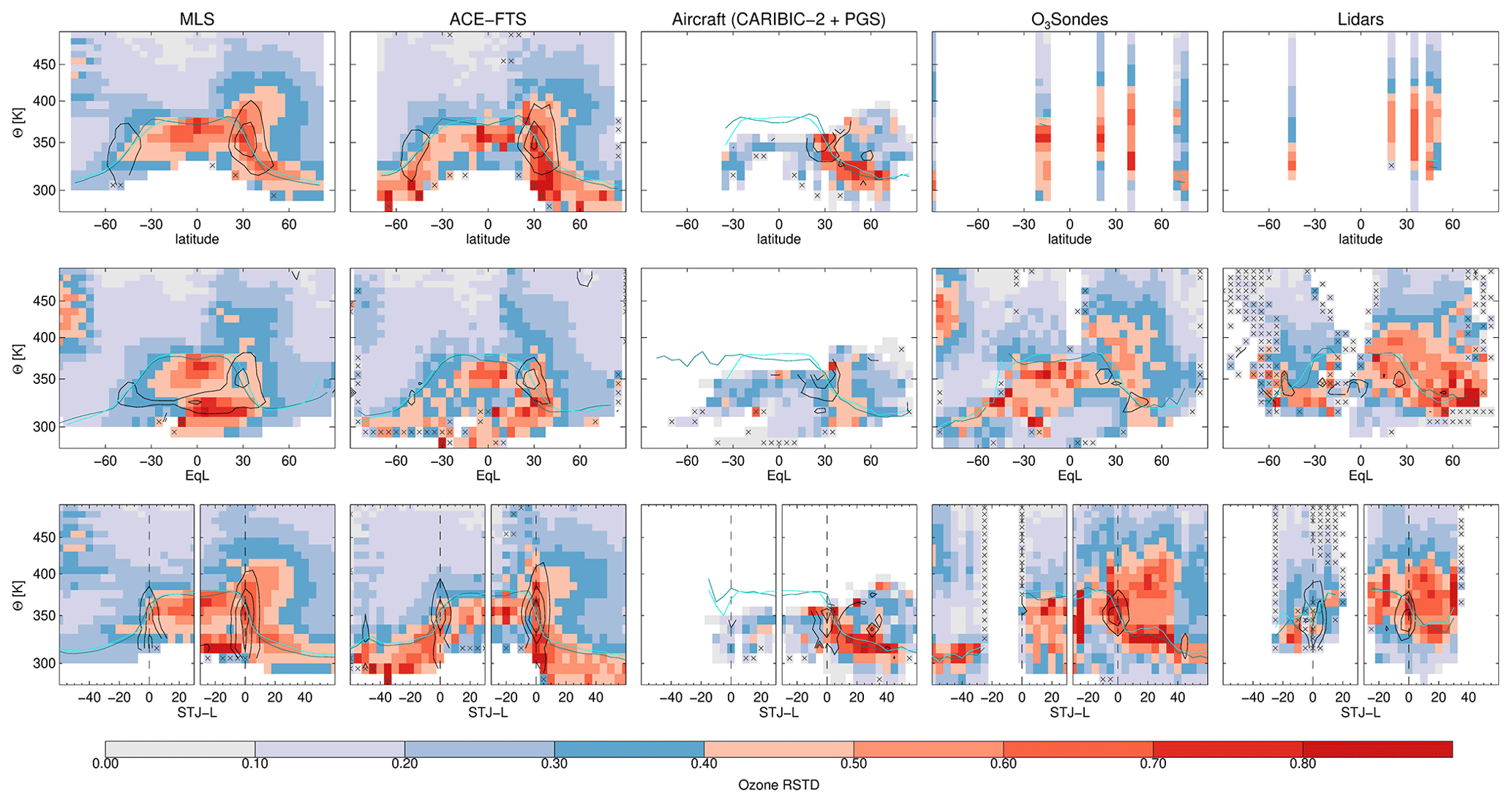
Figure 7 shows the influence on the RSTD of using different horizontal coordinates with potential temperature as the vertical coordinate. The similarity between binning in latitude and binning in STJ-referenced latitude in the MLS and ACE-FTS panels is striking, though the STJ-L panels do show variability along the STJ, with a narrower peak (especially for ACE-FTS). This similarity likely arises from the relatively dense sampling of these datasets and the climatological averaging; it also likely arises partly from the fact that the jets have a strong influence on transport only in the region within about 20–30° latitude of the jet, meaning that distributions are expected to be very similar away from the jets. A similar effect is seen for the aircraft data, albeit with slightly higher RSTD values in the extratropics, again suggesting that the limited latitude region of influence of the jets is an important factor.

For MLS, ACE-FTS, and the aircraft datasets, binning in equivalent latitude leads to a reduction in the RSTD. For example, the lobe of the high RSTD above the northern STJ in latitude and at 0° in the STJ-L coordinate system is greatly reduced when binning the data using equivalent latitude. This is also evident in the ozonesonde and lidar datasets, which show higher RSTD values when binned in latitude with respect to the STJ compared to binning using equivalent latitude. The high RSTD values are greatly reduced when using equivalent latitude, which accounts for the different dynamical regimes and isentropic PV gradients away from the STJ. This illustrates that a portion of the variability is related to reversible processes, in this case primarily the undulation of planetary and synoptic-scale waves. In contrast, binning with respect to the STJ leads to pronounced RSTD values at the jet core location (i.e., 0° with respect to the STJ) due to the strong ozone gradient across the jet, but further from the jet, the variability is higher than that observed with the other horizontal coordinates.

Overall, Fig. 7 indicates that all datasets benefit from the use of equivalent latitude. This coordinate implicitly includes the dynamical tropopause and accounts for dynamics on the typical timescale of planetary wave activity by accounting for the reversible part of the planetary-wave-induced air mass excursions in the mean, especially in the lower stratosphere. However, it is important to exercise caution when using equivalent-latitude coordinates in the upper troposphere. Adiabatic PV conservation is violated, particularly by phase transitions of water, regional turbulence (especially near jet cores), radiative cooling in anticyclones (e.g., Zierl and Wirth, 1997) or above clouds (e.g., Kunkel et al., 2016), and the absence of a connected circumpolar transport barrier (e.g., Manney et al., 2011; Pan et al., 2012; Jin et al., 2013; Kaluza et al., 2021). STJ-relative coordinates are more appropriate for processes in the region immediately surrounding the jet and for studies where identifying and quantifying the strength and sharpness of the jet is critical.

4 Discussion

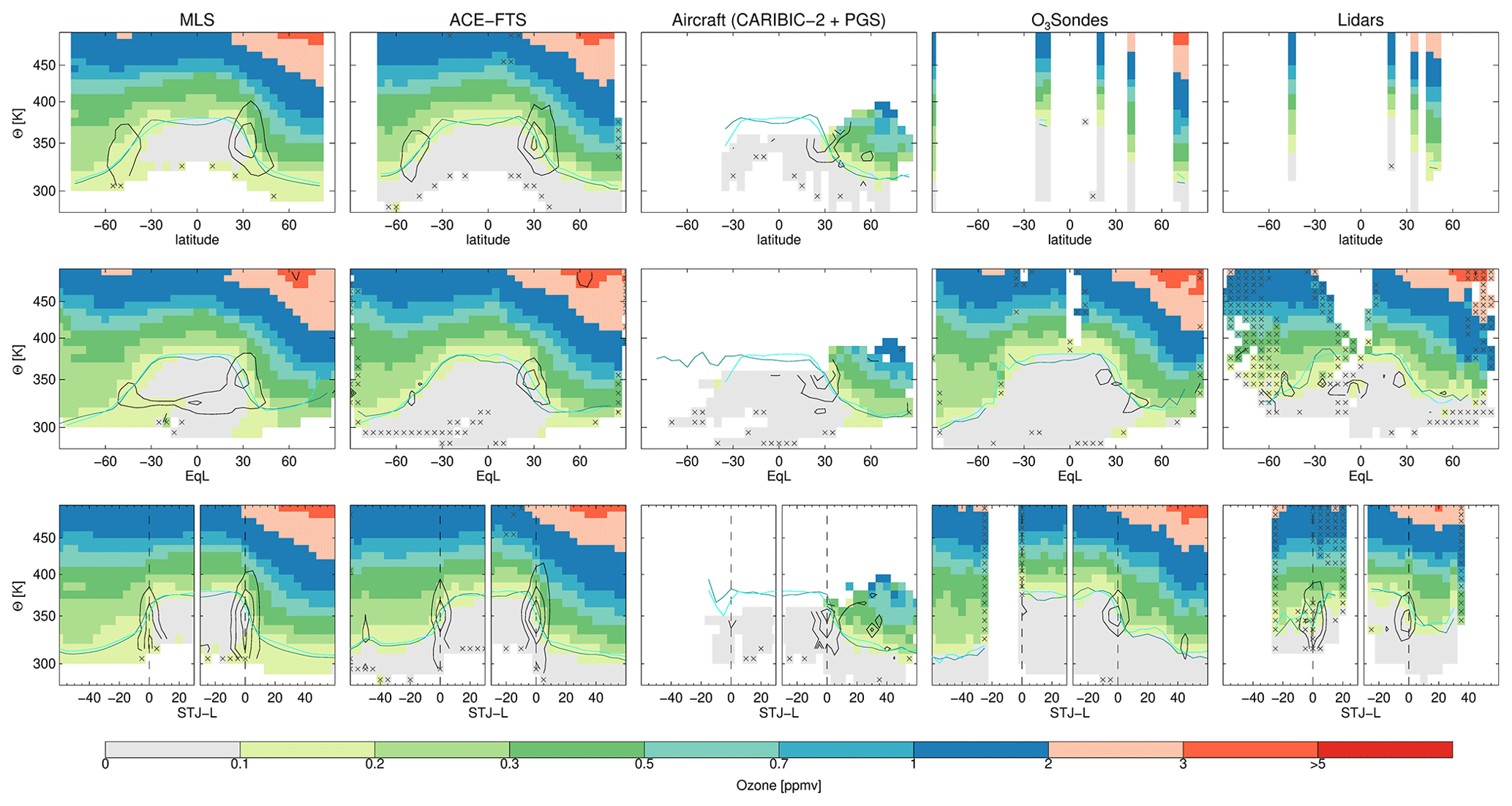
We now discuss the DJF RSTD for MLS (Fig. 8), ozonesondes (Fig. 9), and aircraft measurements (Fig. 10) to illustrate the differences between the various coordinate systems. These datasets were chosen to exemplify satellite observations (MLS) with relatively coarse vertical and horizontal resolutions but with global coverage as well as examples of in situ data with fine vertical resolution (ozonesondes) and horizontal resolution (aircraft) but with limited geographical coverage. The equivalent figures for ACE-FTS and lidars are shown in the Appendix (Figs. C1 and C2).

Despite their different sampling and data densities, all datasets show broad areas of agreement (i.e., consistency in the change) when comparing the various binned coordinate systems in Figs. 8, 9, and 10. Comparing the typically used vertical coordinates (altitude, pressure, and potential temperature) versus latitude, equivalent latitude, and latitude relative to the STJ (top three rows in these figures), all the datasets show a significant reduction in binned variability in the equivalent latitude–potential temperature coordinate system. For example, the binned variability directly at the extratropical tropopause (including the subtropics) is greatly reduced. Further, the lobes of variability above the northern STJ as seen in MLS (Fig. 8) almost disappear in this coordinate system.

This result may not be too surprising since equivalent latitude and potential temperature constitute a purely adiabatic coordinate system combining isentropes (i.e., adiabats) with PV, which is materially conserved for adiabatic and frictionless flow. Equivalent latitude facilitates identification of a reversible adiabatic transport component (which can be appropriately accounted for using suitable coordinates) and a non-adiabatic component related to irreversible mixing. The latter cannot be fully accounted for by coordinate mapping and constitutes part of natural atmospheric variability. In contrast, minimizing the impact of the former is contingent upon the selection of suitable coordinates.

Figure 8 Overview of the MLS DJF (2005–2018) ozone relative standard deviation. Cyan lines show the 4.5 PVU dynamical tropopause and teal lines the WMO (thermal) tropopause (dotted teal lines show the secondary thermal tropopause). The black contours show wind speed values of 30, 40, and 50 m s⁻¹.

Figure 9 As in Fig. 8 but displaying the ozonesonde relative standard deviation.

Figure 10 As in Fig. 8 but displaying the aircraft relative standard deviation.

Regarding tropopause-relative coordinates, we subdivided the data into two categories using geometric altitude and potential temperature relative to the tropopause. Across all the datasets, the use of tropopause-relative altitude coordinates consistently results in higher binned variability than tropopause-relative potential temperature coordinates, regardless of the horizontal coordinate used. This again highlights the quasi-isentropic stratospheric distribution of ozone. Overall, the binned variability is lower for all the horizontal coordinates when using either the 2 PVU tropopause or the 4.5 PVU tropopause as a reference than when using the WMO tropopause. Further, the 2 PVU relative coordinate in general leads to higher binned variability in the subtropics than the 4.5 PVU coordinate but with very similar binned variability elsewhere. The enhanced tropical variability when using the 2 PVU tropopause is in line with the findings of Hoinka (1998) and Kunz et al. (2011a), which concluded that the subtropical tropopause is better represented by the ∼ 4–5.5 PVU surfaces, depending on the season.

As discussed in Sect. 3, double tropopauses associated with the STJ manifest themselves as regions of enhanced ozone variability (around 30° S and 30° N) since a vertical coordinate with respect to the primary tropopause cannot account for mixing measurements taken relative to the lower (primary) and upper (secondary) tropopause and air mass references with tropospheric and stratospheric origins that are quasi-horizontally advected between the primary and secondary tropopauses. These lobes of binned variability are somewhat reduced when using STJ-referenced latitude. However, away from the STJ core, the binned variability increases since the jet is a primary factor (i.e., a transport barrier) in controlling the flow only in a narrow latitude band around the jet core, and thus the flow away from this region is better represented by a dynamical coordinate such as equivalent latitude.

Binning in an equivalent latitude–tropopause-referenced coordinate results in high binned variability near the South Pole during DJF (and near the North Pole during JJA; see the Appendix). In fact, it leads to higher binned variability than using latitude or STJ latitude at all times. This is related to the thermal structure in the polar regions, where both WMO and dynamical tropopauses are often ill-defined and/or very broad (e.g., Bethan et al., 1996; Zängl and Hoinka, 2001; Wilcox et al., 2012).

Regarding vertical STJ coordinates, the data are again shown for coordinates relative to both altitude and potential temperature. As expected, across all the datasets, the use of STJ coordinates relative to altitude results in larger RSTD values than for STJ coordinates relative to potential temperature, regardless of the horizontal coordinate used. Examining the RSTD values across the coordinate systems which use STJθ as the vertical coordinate, it is evident that the binned variability is minimized when using STJ-L as the horizontal coordinate. That is, referring to the STJ in both the vertical and horizontal leads to the lowest binned variability within the STJ-based coordinates.

All of the findings discussed in this section also hold for ACE-FTS and lidar datasets (see Figs. C1 and C2) as well as for the other seasons (see Figs. D1–D5 for JJA examples).

To further quantify the impact of using the various coordinate systems on variability, we use the binned climatological values of latitude and pressure in the different coordinate systems to remap the variability to the “traditional” latitude–pressure coordinate system. The accuracy of this remapping depends on how representative the climatological latitude and pressure values are in the different coordinate systems. Consequently, it only offers a broad overview of the impacts of these coordinate systems. The difference between the RSTD of the reference coordinate system (RSTD_ref) and that of each of the remapped climatologies (RSTD_clim) is calculated as

$$\begin{array}{}\text{(2)}& {\mathrm{RSTD}}_{\mathrm{diff}}={\displaystyle \frac{{\mathrm{RSTD}}_{\mathrm{clim}}-{\mathrm{RSTD}}_{\mathrm{ref}}}{{\mathrm{RSTD}}_{\mathrm{ref}}}},\end{array}$$

which yields a direct metric for assessing the effect of these coordinate systems on the binned variability.

Figure 11 displays the result of remapping and comparing the MLS DJF data. Notably, the use of equivalent latitude–potential temperature (EqL $/\mathit{\theta }$) coordinates leads to the most substantial reduction in binned variability across the upper troposphere and lowermost stratosphere. Equivalent latitude effectively accounts for the reversible short-term variability at the extratropical tropopause, while potential temperature accounts for the vertical variability of isentropic surfaces and thus isentropic vertical displacement of air parcels. To highlight this further, Fig. E1 displays the same MLS DJF data comparison using the climatological values of equivalent latitude and θ, i.e., remapping into EqL $/\mathit{\theta }$. In all the other coordinates, there is enhanced binned variability, except in small regions, emphasizing the global utility of this coordinate pairing. Given the importance of equivalent latitude, other methods to calculate it (e.g., Añel et al., 2013) could be explored in the future.

Figure 11 also highlights that any tropopause-based coordinate leads to reduced binned variability around the tropopause, consistent with the results of Hegglin et al. (2009). It is important to note that, at greater distances from the respective tropopauses, tropopause coordinates in altitude tend to increase variability for all horizontal coordinates. This confirms earlier results by Hegglin et al. (2008) and indicates that using tropopause-based altitude coordinate systems may not be physically meaningful farther away from the tropopauses. Similarly, STJ coordinates lead to reduced binned variability only around the STJ, consistent with the results of Manney et al. (2011).

The reduction in variability observed in tropopause-based coordinates relative to potential temperature, especially in the winter hemisphere when the Brewer–Dobson circulation dominates vertical movement via advection, supports this interpretation (e.g., Hoor et al., 2004; Hegglin et al., 2006). Unlike altitude, potential temperature accounts for at least some of the large-scale adiabatic movements driven by the stratospheric circulation in the deeper stratosphere on shorter timescales (e.g., Harzer et al., 2023). Finally, some of this enhanced variability in all the tropopause-based coordinates is generally further reduced when using latitude with respect to the STJ.

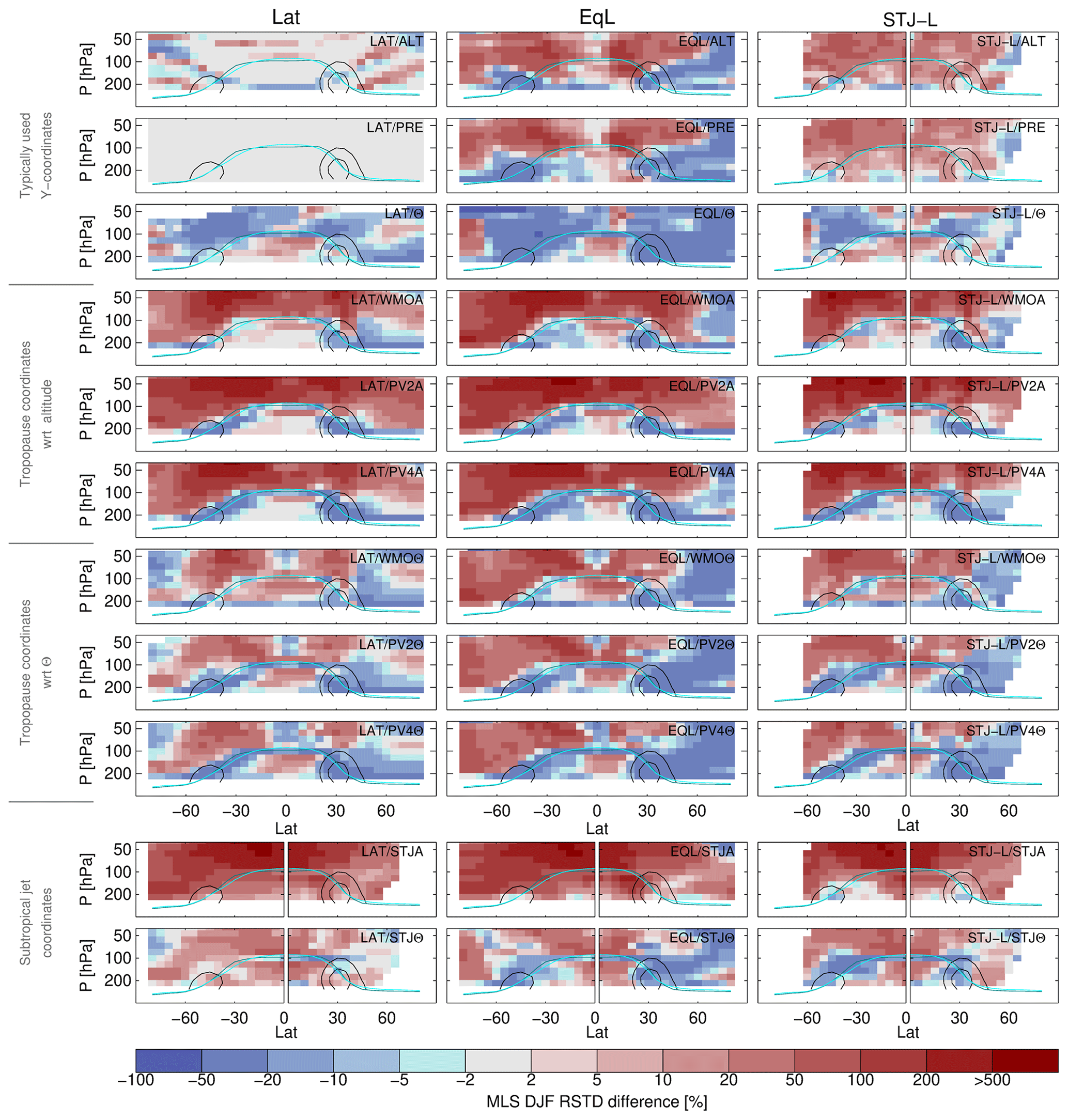
Figure 11 Relative standard deviation changes in different coordinates in comparison to binning in latitude and pressure. The red colors indicate an increase in binned variability, while the blue colors denote a reduction in binned variability.

5 Summary

As part of the OCTAV-UTLS SPARC activity, we have mapped multiplatform ozone datasets to different coordinate systems to systematically evaluate the influence of these coordinates on the binned climatological variability, unifying the disparate work of numerous prior studies on individual coordinate system variability in the most complete assessment of this topic that we are aware of. Coordinate systems that do not consider transport barriers can induce artificial variability when binning across ozone gradients at transport barriers, increasing the binned variability. By comparing the relative standard deviation in different coordinate systems, we evaluated the ability of each coordinate to account for variations arising from changes in the subtropical upper-tropospheric jet, changes in tropopause height, and wave-induced air parcel displacements. We thus evaluated the ability of each coordinate system to identify different regimes separated by transport barriers and to group air parcels appropriately into those regimes.

We found the following:

• Across all the datasets, referring to the tropopause or STJ core in the vertical leads to greater binned variability in altitude-based coordinates compared to potential temperature-based coordinates, irrespective of the horizontal coordinate used. This highlights the largely quasi-isentropic distribution of upper-tropospheric and lower-stratospheric ozone.

• Any tropopause-based coordinate (compared to commonly used coordinates such as altitude and pressure) leads to reduced binned variability just around the tropopause, consistent with previous studies. However, higher variability is seen in tropopause-based coordinates at some distances from the respective tropopauses.

• The binned variability is lower for all the horizontal coordinates when using either the 2 PVU or 4.5 PVU tropopause as a reference than when using the WMO tropopause.

• STJ-relative latitude leads to somewhat reduced binned variability in a narrow latitude band around the STJ core; farther from the STJ, equivalent latitude better represents the air parcels' movement.

• The use of equivalent latitude–potential temperature coordinates leads to the most substantial reduction in binned variability across the UTLS through all the datasets and all the seasons. Because this coordinate system uses PV on isentropic surfaces and PV is conserved for adiabatic frictionless flow, the transport of tracers follows this coordinate system.

These conclusions were drawn using a variety of ozone measurements (i.e., ozonesondes, lidars, and satellite and in situ aircraft measurements) with a plethora of vertical and horizontal resolutions as well as sampling characteristics. Therefore, we anticipate that these results will be applicable to other datasets not included in this study, such as OMPS, OSIRIS, IAGOS-CORE, and additional ozonesondes and lidar data available elsewhere.

We note that each coordinate system has its strengths and weaknesses, and thus different coordinate systems may be most effective for times and regions dominated by variability from different atmospheric processes. In this study, we identified coordinate systems that most help to reduce binned variability over broad regions in an effort to facilitate more robust UTLS composition trend analyses. The use of multiple datasets with different samplings and resolutions enables us to identify commonalities among them, ensuring conclusions that are independent of the specific measurement techniques. We are aware that several questions regarding the binned variability are still open, and some of them will be addressed in upcoming studies. For example, a future OCTAV-UTLS study will evaluate the impact of using those coordinates that most reduce binned variability in quantification of long-term ozone trends. Another study will analyze how differences in sampling patterns and resolution (both vertical and horizontal) can affect the representation of the datasets as well as the trend quantification.

Appendix A: Abbreviations and symbols used in this study

Table A1 Abbreviations and symbols used in this study.

^a Polar stratosphere in a changing climate. ^b Investigation of the life cycle of gravity waves. ^c Seasonality of air mass transport and origin in the lowermost stratosphere.

Appendix B: Number of measurements per bin

Figure B1 As in Fig. 2 but displaying the number of measurements (the count) in each bin for several coordinate systems.

Appendix C: DJF variability for ACE-FTS and lidars

Figure C1 As in Fig. 8 but displaying the ACE-FTS ozone relative standard deviation.

Figure C2 As in Fig. 8 but displaying the lidar ozone relative standard deviation.

Appendix D: JJA variability

Figure D1 As in Fig. 8 but displaying the MLS JJA ozone relative standard deviation.

Figure D2 As in Fig. 9 but displaying the ozonesonde JJA ozone relative standard deviation.

Figure D3 As in Fig. 10 but displaying the aircraft JJA ozone relative standard deviation.

Figure D4 As in Fig. C1 but displaying the ACE-FTS JJA ozone relative standard deviation.

Figure D5 As in Fig. C2 but displaying the lidar JJA ozone relative standard deviation.

Appendix E: Variability with respect to EqL $/\mathit{\theta }$

Figure E1 As in Fig. 11 but in comparison to binning in equivalent latitude and potential temperature.