Does the Asian summer monsoon play a role in the stratospheric aerosol budget of the Arctic?

The Asian summer monsoon has a strong convectional component with which aerosols are able to be lifted up into the lower stratosphere. Due to usually long lifetimes and long-range transport aerosols remain there much longer than in the troposphere and are also able to be advected around the globe. Our aim of this study is a synergy between simulations by Chemical Lagrangian Model of the Stratosphere (CLaMS) and KARL (Koldewey Aerosol Raman Lidar) at AWIPEV, Ny-Ålesund in the Arctic, by comparing CLaMS results with exemplary days of lidar measurements as well as analyzing the stratospheric aerosol background. We use global three-dimensional Lagrangian transport simulations including surface origin tracers as well as back trajectories to identify source regions of the aerosol particles measured over Ny-Ålesund. We analyzed lidar data for the year 2021 and found the stratosphere generally clear, without obvious aerosol layers from volcanic eruptions or biomass burnings. Still an obvious annual cycle of the backscatter coefficient with higher values in late summer to autumn and lower values in late winter has been found. Results from CLaMS model simulations indicate that from late summer to early autumn filaments with high fractions of air which originate in South Asia – one of the most polluted regions in the world – reach the Arctic at altitudes between 360 and 380 K potential temperature. We found a coinciding measurement between the overpass of such a filament and lidar observations, and we estimated that backscatter and depolarization increased by roughly 15 % during this event compared to the background aerosol concentration. Hence we demonstrate that the Asian summer monsoon is a weak but measurable source for Arctic stratospheric aerosol in late summer to early autumn.

1 Introduction

Already in 1960 Junge et al. (1961a) characterized some basic properties of stratospheric aerosols like size distribution, physical structure and chemical composition up to 30 km altitude. Stratospheric aerosols can be either long-range transported, injected from the troposphere or even directly created in the stratosphere and has a high sulfuric content (Junge et al., 1961a; Kremser et al., 2016), and they have a big impact on the local ozone layer but also on the radiative budget with a cooling factor due to additional scattering of direct solar radiation. Already Junge et al. (1961a) pointed out different mechanisms acting on stratospheric aerosols, like horizontal mixing due to large-scale exchange by intrusions through the tropopause, meridional and hemispheric circulations, or gravitational settling of particles determined by Stokes' law. Junge et al. (1961a) and Murphy et al. (2021) found in stratospheric in situ measurements a remarkable constant layer of particles in the accumulation mode (from 0.1 to 1 µm). Particles larger than that are created by oxidation of H₂S and SO₂ in the layer they are found in. Strong zonal winds in the stratosphere lead to a fast homogenization of aerosols, while vertical and meridional transport is controlled by the Brewer–Dobson circulation (BDC) (Holton et al., 1995; Butchart, 2014). The BDC is characterized by a meridional transport from rising air at the tropics towards high latitudes and a quasi-horizontal mixing over the extra-tropics (McIntyre and Palmer, 1983). This circulation and mixing control not only long-range transport (Shepherd, 2002) but also aging of aerosols (Waugh and Hall, 2002).

As Junge et al. (1961a) found out, lifetimes of aerosols in the lower stratosphere are on the order of magnitude of several hundred days and can easily be advected to higher latitudes and distributed over the entire globe. Due to the absence of water vapor in the stratosphere aerosol removal by precipitation does not take place. Therefore they are usually removed by sedimentation.

During the first 4 years of CALIPSO measurements (Cloud–Aerosol Lidar and Infrared Pathfinder Satellite Observations) an Asian tropopause aerosol layer (ATAL) was found during the Asian summer monsoon season at altitudes of 13 to 18 km, equivalent to 360 to 420 K potential temperature, while the Junge layer is usually at around 20 km (Junge et al., 1961b). With usually occurring depolarization values of up to 5 % and backscattering ratios of around 1.10 to 1.15, this layer is driven by an enhancement of background aerosol (Vernier et al., 2011). While overall the amount of non-sulfate aerosol or anthropogenic sulfur dioxide is difficult to assess (Kremser et al., 2016), the ATAL might be responsible for about 15 % of the aerosol content in the Northern Hemisphere. This is comparable to all volcanic eruptions from 2000 to 2015 (Yu et al., 2017) and within the order of magnitude of the estimated amount of ejected SO₂ during the Pinatubo eruption in 1991 (Andersson et al., 2015; Kremser et al., 2016; Quaglia et al., 2023). Chemical in situ measurements revealed that the ATAL mainly consists of secondary substances containing nitrate, ammonium, sulfate and organics and is therefore more diverse in its chemical composition than the Junge layer (Appel et al., 2022).

The Asian summer monsoon has very strong deep convection, where updrafts of 4 m s⁻¹ up to altitudes of 400 K are common (Wang, 2004; Randel et al., 2010; Bian et al., 2020), which allow both gas-phase aerosol precursors and aerosol particles from surface sources to reach the stratosphere (Vogel et al., 2019; Brunamonti et al., 2018; Hanumanthu et al., 2020). Several studies confirm that the horizontal transport out of the Asian monsoon anticyclone has an impact on the extratropical lower stratosphere of the Northern Hemisphere (e.g., Vogel et al., 2016; Yu et al., 2017; Yan et al., 2024). Besides volcanic activities, anthropogenic emissions make a large contribution to the total concentration of aerosol with sulfuric components. As Notholt et al. (2005) and Klimont et al. (2013) show, the sulfur emission of Europe, North America and the former Soviet Union is constantly decreasing, while the emission drastically increases in Southeast Asia, where also the very effective uplift of pollution, gas-phase aerosol precursors and aerosol particles in the stratosphere by the Asian summer monsoon takes place. Some observational evidence of an increasing of stratospheric aerosols globally was found by Vernier et al. (2011), who used observations by Cloud–Aerosol Lidar and Infrared Pathfinder Satellite Observations (CALIPSO) to reveal that the ATAL near 16 km in June to September is associated with the Asian monsoon anticyclone.

Using the CLaMS model (Chemical Lagrangian Model of the Stratosphere) and aircraft measurements over Europe and the northern Atlantic, horizontal pathways out of the Asian monsoon anticyclone were found exporting young polluted air masses eastward into the northern extratropical lower stratosphere within several weeks (e.g., Vogel et al., 2016; Wetzel et al., 2021; Lauther et al., 2022). In particular source regions of anthropogenic short-lived species such as CH₂Cl₂ emission are mainly located in Asia; therefore CH₂Cl₂ is a very good marker for transport out of the Asian monsoon anticyclone into the northern extratropical stratosphere (Lauther et al., 2022). The good linkage between CLaMS surface origin tracers and measured pollution tracers such as CH₂Cl₂ and PAN (Wetzel et al., 2021; Lauther et al., 2022) shows that CLaMS is very well suited for analyzing aerosol transport out of the ATAL.

Furthermore, aerosols originating from extended boreal biomass burnings especially in Russia and North America have been seen in the Arctic summer stratosphere at different sights and years in the Arctic (Zielinski et al., 2020; Ohneiser et al., 2021; Cheremisin et al., 2022). According to satellite-based studies of global extinction results wildfires can only be found in the lowermost part of the stratosphere with a relatively short lifetime (Thomason and Knepp, 2023). Therefore, the annual cycle with its natural variability and the origin of the Arctic stratospheric aerosol layer is important.

Currently stratospheric aerosol represents an interesting research topic as already several studies have analyzed a potential impact of stratospheric aerosol injections on geoengineering (e.g., Irvine and Keith, 2020; Cheng et al., 2022) to counteract the global rise in temperature. As Sun et al. (2020) point out, the impact of an injection of sulfuric aerosols into the stratosphere will change globally the incoming radiation but also the precipitation. Additionally, the effect will be different depending on the location of injection as well as the amount.

However, clearly all potential impacts on the climate system need to be understood prior to the execution of such a costly and risky environmental endeavor. To minimize impacts of precipitation suppression some authors favor aerosol injection into the Arctic summertime stratosphere (Lee et al., 2021). It is therefore important to understand the existing contribution of the un-modified stratospheric aerosol content in the Arctic, which may also originate from the Asian summer monsoon. As a first step we look into the seasonal variability in the Arctic stratospheric background aerosol impacted by the Asian summer monsoon.

Therefore we use model simulations to identify the contribution of the Asian summer monsoon to air masses detected by lidar measurements in the Arctic. For this study we focus on the year 2021, since it was a year with a statistically average number of biomass burnings in the Northern Hemisphere, and we have a qualitatively good lidar data set for every month of the year. In Sect. 2.1 we describe the instrument sight, followed by a short overview of the lidar KARL (Koldewey Aerosol Raman Lidar; see Sect. 3.3), radiosondes in Sect. 2.3, the model CLaMS (see Sect. 2.4) and the satellite MODIS in Sect. 2.5. We present an overview of basic stratospheric aerosol properties above our Arctic site in Sect. 2.2 which shows a weak but clear annual cycle. Further we show the output of a Lagrangian chemical transport model in Sect. 3.5 which shows the occurrences of air which originated in the Asian summer monsoon region over the Arctic. The discussion of the results will be presented in Sect. 4, and the conclusion will follow in Sect. 5.

2 Measurement site, instrument and model

2.1 Arctic measurement site: Ny-Ålesund

The observation site in Ny-Ålesund is located in the European Arctic (78.923° N, 11.928° E) on the northwest coast of the archipelago of Svalbard along the shore of Kongsfjord, which is orientated in a southeast to northwest direction on the west coast of Svalbard (Fig. 1).

Figure 1 Map of the vicinity of Ny-Ålesund, Kongsfjord, and its location in Europe. Sources: https://geokart.npolar.no/Html5Viewer/index.html?viewer=Barentsportal (last access: 23 April 2024), courtesy of Norsk Polarinstitutt and https://de.wikipedia.org/wiki/Datei:Europe_on_the_globe_(red).svg (last access: 23 April 2024).

2.2 KARL – Koldewey Aerosol Raman Lidar

2.2.1 Description of KARL

The lidar measurements were performed at the German–French AWIPEV research base in Ny-Ålesund, Svalbard, by the “Koldewey Aerosol Raman Lidar” (KARL). This system consists of a Spectra 290/50 Nd:YAG laser, which emits a laser beam at 355, 532 and 1064 nm with 50 Hz and 200 mJ per pulse and color vertically into the atmosphere. The backscattered photons are collected by a 70 cm telescope with a field of view of about 2 mrad in the elastic colors as well as in the Raman-scattered signals at N₂ at 387 and 607 nm. Data recording is done via Hamamatsu photomultipliers and Licel transient recorders with 7.5 m resolution. Full overlap is reached at about 700 m altitude. A more detailed description of the instrument is given by Hoffmann (2011). The aerosol backscatter coefficient β^aer(λ) [(m sr)⁻¹] and the aerosol extinction coefficient α^aer(λ) [m⁻¹] were calculated following the principle of Ansmann et al. (1992). For better readability and simplicity we use β(λ):=β^aer(λ) and α(λ):=α^aer(λ) in the following, if not stated otherwise. The lidar ratios, $\mathrm{LR}=\frac{{\mathit{\alpha }}^{\mathrm{aer}}\left(\mathit{\lambda }\right)}{{\mathit{\beta }}^{\mathrm{aer}}\left(\mathit{\lambda }\right)}$ [sr], for the other wavelengths were chosen as LR₃₅₅=50 sr for the troposphere and LR₃₅₅=70 sr in the stratosphere and for λ=532 nm LR₅₃₂=36 sr and LR₅₃₂=42 sr in the troposphere and stratosphere, respectively, if not stated otherwise. High values of LR indicate highly absorbing particles and are therefore mostly related to the refractive index but also to shape and size. The fact that we found LR₅₃₂<LR₃₅₅ in the stratosphere was derived by our lidar data via two conditions: same backscatter at different wavelengths for (tropospheric) cirrus clouds and the same gradients for the aerosol backscatter in clear layers of the troposphere. Since we do not expect rapid changes in the physical and chemical composition of aerosols in the lower stratosphere and to reduce the uncertainty due to noise, especially during polar day, we chose a temporal and spacial resolution of 60 min and 150 m for the elastic profiles at 355 and 532 nm. Both signals can always be evaluated up to almost 30 km height.

2.2.2 Parameters and fundamental equations

It is well known from Klett (1981, 1985) that the solution of the elastic lidar equation is

$$\begin{array}{}\text{(1)}& P\left(z\right)=\mathrm{Const}\cdot {\displaystyle \frac{{\mathit{\beta }}^{\mathrm{tot}}\left(z\right)}{z^{\mathrm{2}}}}\cdot \exp \left(-\mathrm{2}\underset{z_{\mathrm{0}}}{\overset{z}{\int }}{\mathit{\alpha }}^{\mathrm{tot}}\left(\widehat{z}\right)\mathrm{d}\widehat{z}\right),\end{array}$$

where P(z) is the signal power at a given height z, Const a constant determined by the instrument itself and its setup, ${\mathit{\beta }}^{\mathrm{tot}}\left(z\right)={\mathit{\beta }}^{\mathrm{aer}}+{\mathit{\beta }}^{\mathrm{Ray}}$ the total backscatter signal, and ${\mathit{\alpha }}^{\mathrm{tot}}\left(z\right)={\mathit{\alpha }}^{\mathrm{aer}}+{\mathit{\alpha }}^{\mathrm{Ray}}+{\mathit{\alpha }}^{\mathrm{abs}}$ the total extinction, depending on the choice of a lidar ratio and on the choice of a boundary condition. The extensions “aer”, “Ray” and “abs” are the contributions of aerosols and Rayleigh scattering as well as the absorption by trace gases. β^aer needs to be prescribed at a certain altitude. Klett (1981, 1985) pointed out that the solution is stable and less critically dependent on the assumed boundary condition, when the integration is done “backwards”: from large distances back to the lidar.

We set the boundary condition, ϵ, in the altitude interval from 27 to 30 km for March to November. In winter times, polar stratospheric clouds (PSCs) might occur at this altitude (Tritscher et al., 2021), so we lowered the fitting range to 24 to 27 km. No PSCs were found in our data set after this adjustment. In this altitude range we assume that the average total backscatter coefficient in that interval is ${\mathit{ϵ}}_{\mathrm{532}}=\mathrm{1.10}\cdot {\mathit{\beta }}^{\mathrm{Ray}}$ and ${\mathit{ϵ}}_{\mathrm{355}}=\mathrm{1.05}\cdot {\mathit{\beta }}^{\mathrm{Ray}}$ for parallel and perpendicular. The signal-to-noise ratio, SNR, is calculated following Eq. (2).

$$\begin{array}{}\text{(2)}& \mathrm{SNR}\left(z\right)={\displaystyle \frac{P\left(z\right)}{P_{\mathrm{err}}\left(z\right)}}={\displaystyle \frac{P\left(z\right)}{\sqrt{P\left(z\right)}+P_{\mathrm{bgrd}}}}\end{array}$$

Here P_err is the estimated noise profile and P_bgrd the averaged signal in an altitude range, which is dominated by electronic noise and background light in an altitude range of 52 to 60 km. The lidar signal P(z) is given in the units of “counts” like in the photo-counting channels. This altitude range has a sufficiently small median signal-to-noise ratio. Therefore it is valid to assume there is just noise in the signal. The SNR is shown in Table 1 at an altitude of 20 km for the different wavelengths and directions of polarization.

Table 1 Mean of the signal-to-noise ratio for all emitted wavelengths and directions of polarization at 20 km altitude.

With these high values of signal-to-noise ratio we conclude that the data set is sufficiently good for a further evaluation of observations of physical features in the lower stratosphere. Since the depolarization is very low (see Sect. 3.3.2), the signal is much weaker than for the parallel polarized light, and therefore the SNR is generally smaller. Due to the small SNR at 20 km the signal of λ=1064 nm is neglected for this study.

From the lidar data we derive the following quantities: the lidar ratio LR, aerosol depolarization δ^aer(λ) and the backscatter color ratio CR were calculated following Eq. (3):

$$\begin{array}{}\text{(3)}& \begin{array}{rl}& \mathrm{LR}\left(\mathit{\lambda }\right)={\displaystyle \frac{{\mathit{\alpha }}^{\mathrm{aer}}\left(\mathit{\lambda }\right)}{{\mathit{\beta }}^{\mathrm{aer}}\left(\mathit{\lambda }\right)}},{\mathit{\delta }}^{\mathrm{aer}}\left(\mathit{\lambda }\right)={\displaystyle \frac{{\mathit{\beta }}_{⟂}^{\mathrm{aer}}\left(\mathit{\lambda }\right)}{{\mathit{\beta }}_{\parallel }^{\mathrm{aer}}\left(\mathit{\lambda }\right)}},\\ & \mathrm{CR}({\mathit{\lambda }}_{\mathrm{1}},{\mathit{\lambda }}_{\mathrm{2}})={\displaystyle \frac{{\mathit{\beta }}^{\mathrm{aer}}\left({\mathit{\lambda }}_{\mathrm{1}}\right)}{{\mathit{\beta }}^{\mathrm{aer}}\left({\mathit{\lambda }}_{\mathrm{2}}\right)}}.\end{array}\end{array}$$

Here, ${\mathit{\beta }}_{⟂}^{\mathrm{aer}}$ and ${\mathit{\beta }}_{\parallel }^{\mathrm{aer}}$ are the backscatter coefficients with respect to the perpendicular and parallel laser polarization, respectively, which are measured separately in the elastic 355 and 532 nm channels. For β^aer and δ^aer only 532 and 355 nm signals were used. The color ratio is defined with λ₁<λ₂.

In contrast to the backscatter coefficient, β, the backscatter ratio, R, is dimensionless and does not decrease with increasing height. It is defined as in Eq. (4):

$$\begin{array}{}\text{(4)}& R\left(\mathit{\lambda }\right)={\displaystyle \frac{{\mathit{\beta }}^{\mathrm{tot}}\left(\mathit{\lambda }\right)}{{\mathit{\beta }}^{\mathrm{Ray}}\left(\mathit{\lambda }\right)}}=\mathrm{1}+{\displaystyle \frac{{\mathit{\beta }}^{\mathrm{aer}}\left(\mathit{\lambda }\right)}{{\mathit{\beta }}^{\mathrm{Ray}}\left(\mathit{\lambda }\right)}}.\end{array}$$

An ideal, aerosol-free atmosphere would have R=1, which increases with stronger pollution. The parameter R is therefore a good indication for aerosol existence.

With the ERA5 reanalysis data from Hoffmann and Spang (2021) the mean height of the tropopause was found at an average height of 9137 m with a standard deviation of 775 m at the study site of Ny-Ålesund during the lidar measurement time and will be further discussed in Sect. 3.2. To investigate the properties of stratospheric aerosol, we focus on the altitude range between 10 to 15 km; most of the troposphere is neglected and not shown in the plots.

2.2.3 Data quality management of lidar data

For this study, we only used automatically flagged data, which fulfilled the following criteria. Each wavelength and profile is tested and eventually removed individually:

1. elimination of negative or too many (>20) values that are too low (R≤1.003)

2. elimination of artificial values that are too high (${\mathit{\beta }}^{\mathrm{aer}}\left(\mathit{\lambda }\right)\ge \mathrm{5}\times {\mathrm{10}}^{-\mathrm{8}}$ (m sr)⁻¹), when the error and parameter variables are equally large, if more than two-thirds of the data points are not a number or if in more than two-thirds of the cases values of R≥2.0 are reached

3. clouds detected in the troposphere with the criteria of two adjacent data points reaching the limit of $\mathrm{\Delta }\mathit{\beta }=\mathrm{1}\times {\mathrm{10}}^{-\mathrm{4}}$ (m sr)⁻¹.

A qualitatively good profile has to fulfill all of these criteria at the same time. If one is not satisfied, the profile is eliminated out of the further processed data set. These criteria were chosen by manually looking at the data of different times of the year and atmospheric conditions with the aim of finding a good balance between eliminating as many disturbed profiles as necessary and keeping the good ones.

2.3 RS41 radiosondes

At least once a day a radiosonde of the type RS41 by Vaisala is launched from AWIPEV at 11:00 UT. The data are processed according to the standards by the Global Climate Observing System (GCOS) Reference Upper-Air Network (GRUAN). A more detailed description of the radiosondes is given by Maturilli and Kayser (2017). With the quality checked and homogenized data set the Rayleigh atmosphere for the correction of lidar profiles is calculated as well as the tropopause height.

2.4 CLaMS – Chemical Lagrangian Model of the Stratosphere

To analyze the origin of air masses over Ny-Ålesund in 2021, we conducted three-dimensional global simulations with the Chemical Lagrangian Model of the stratosphere (CLaMS;  McKenna et al., 2002b, a; Pommrich et al., 2014, and references therein) as well as CLaMS back-trajectory calculations starting along the lidar measurements. The global model simulations are driven by horizontal winds from ERA5 reanalysis (Hersbach et al., 2020), provided by the European Centre for Medium-Range Weather Forecasts (ECMWF).

We use ERA5 data on 137 vertical model levels up to 0.01 hPa (80 km) but at lower horizontal and time resolutions (referred to as ERA5 1°×1°) (similar to Ploeger et al., 2021; Konopka et al., 2022; Clemens et al., 2024). Here, ERA5 data are truncated to a 1°×1° horizontal grid and a 6-hourly time resolution, whereby the vertical resolution is the same as in the original ERA5 reanalysis (about 0.3 to 0.4 km up to 20 km). ERA5 1°×1° data are a computing-time-saving alternative to the full-resolution ERA5 data and are used for three-dimensional global CLaMS simulations. Vertical velocities are calculated following the diabatic approach by Ploeger et al. (2010). CLaMS uses a hybrid vertical coordinate (ζ). At pressure levels lower than 300 hPa, ζ can be interpreted as potential temperature (θ). Towards higher pressure levels, ζ transforms from an isentropic to a pressure-based orography-following hybrid coordinate. Global three-dimensional CLaMS simulations are based on three-dimensional forward trajectories and a parametrization of small-scale mixing depending on the shear in the large-scale wind flow (e.g., Pommrich et al., 2014).

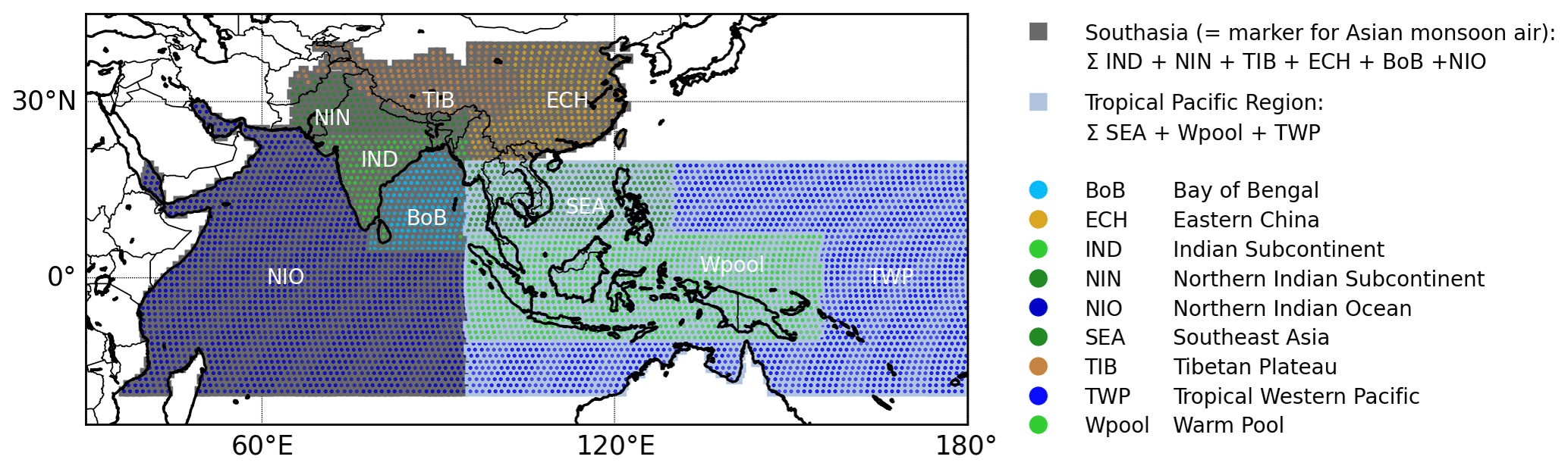
Figure 2 Geographical map showing the location of CLaMS's surface origin tracers in South Asia and the tropical Pacific region. Regions that mostly impact the lidar measurements in Ny-Ålesund are combined into two tracers referred to as “South Asia” and “tropical Pacific region”. The names of the surface origin tracers and their corresponding abbreviations are listed right beside the map.

A three-dimensional CLaMS simulation running from 1 December 2020 until the end of 2021 to cover the entire time period of the year 2021 was performed including artificial surface origin tracers (Vogel et al., 2015, 2016, 2019). The surface origin tracers used in this study cover the entire Earth's surface and are associated with 32 defined regions in the model boundary layer that is about 2 to 3 km above surface considering orography. They are released at the model boundary layer every 24 h and are further transported (advected and mixed) to the free atmosphere. Here in this study it was found that regions in South Asia and in the tropical Pacific region (see Fig. 2) have a major impact on air masses over Ny-Ålesund. The impact of all other regions of the world are minor and are summarized as “residual” and “residual ocean”. Air masses from South Asia are during summer associated with the Asian monsoon circulation and are here used as a marker for Asian monsoon air. Besides continental regions in South Asia, in addition parts of the Indian Ocean and the Bay of Bengal are included in the surface origin tracer for South Asia.

Starting with the onset of the Indian monsoon at the beginning of June, air masses from the Indian Ocean are transported long-range to the north of the Indian subcontinent where they are uplifted into the upper troposphere and lower stratosphere (e.g., Fadnavis et al., 2013; Lau et al., 2018; Nomura et al., 2021; Vogel et al., 2024). These air masses can uptake polluted air while passing over the Indo-Gangetic Plain where anthropogenic emissions are higher compared to other regions in India caused by the dense concentration of industries and the high population (e.g., Fadnavis et al., 2016). Therefore, the tracer for the Indian Ocean and the Bay of Bengal are included in the marker for the Asian monsoon air.

2.5 Moderate Resolution Imaging Spectroradiometer – MODIS

Moderate Resolution Imaging Spectroradiometer (MODIS) is a NASA satellite-based radiometer for Earth observations in 36 different spectral bands reaching from 0.4 to 14.4 µm. It has, depending on the selection of bands, a spatial resolution of 0.25°×0.25° and a temporal resolution of about 2 d. Wildfires are detected by the 4 and 11 µm bands by observing temperature anomalies relative to the background and absolute. In this study only the parameter fire radiative power (FRP) from Aqua and Terra with a gridded spacial resolution of 1 km were used to characterize wildfires. More information can be found at https://modis.gsfc.nasa.gov/data/dataprod/mod14.php (MODIS, last access: 13 June 2024).

3 Results

3.1 Wildfires in North America and Russia

Wildfires occur regularly in the Northern Hemisphere and are a big source for aerosol, which can be lifted by several processes into the stratosphere (Ansmann et al., 2018; Ohneiser et al., 2021). Since air masses coming from Southeast Asia pass Russia and potentially even Canada, the contribution of wildfires has to be considered, i.e., whether the observed increased backscatter is influenced by these or is actually a direct signal from the monsoon region. The area “Russia” is defined within the rectangle by the geographical coordinates 77° N, 31° E and 48° N, 180° E. “Canada” is defined by the corners at 71° N, 170° W and 48° N, 52° W. Active wildfires are combined to monthly overviews. Figure 3 gives an overview of the median and mean FRP measured by MODIS and averaged over all grid cells in the defined regions “Canada” and “Russia” from 2001 to 2022.

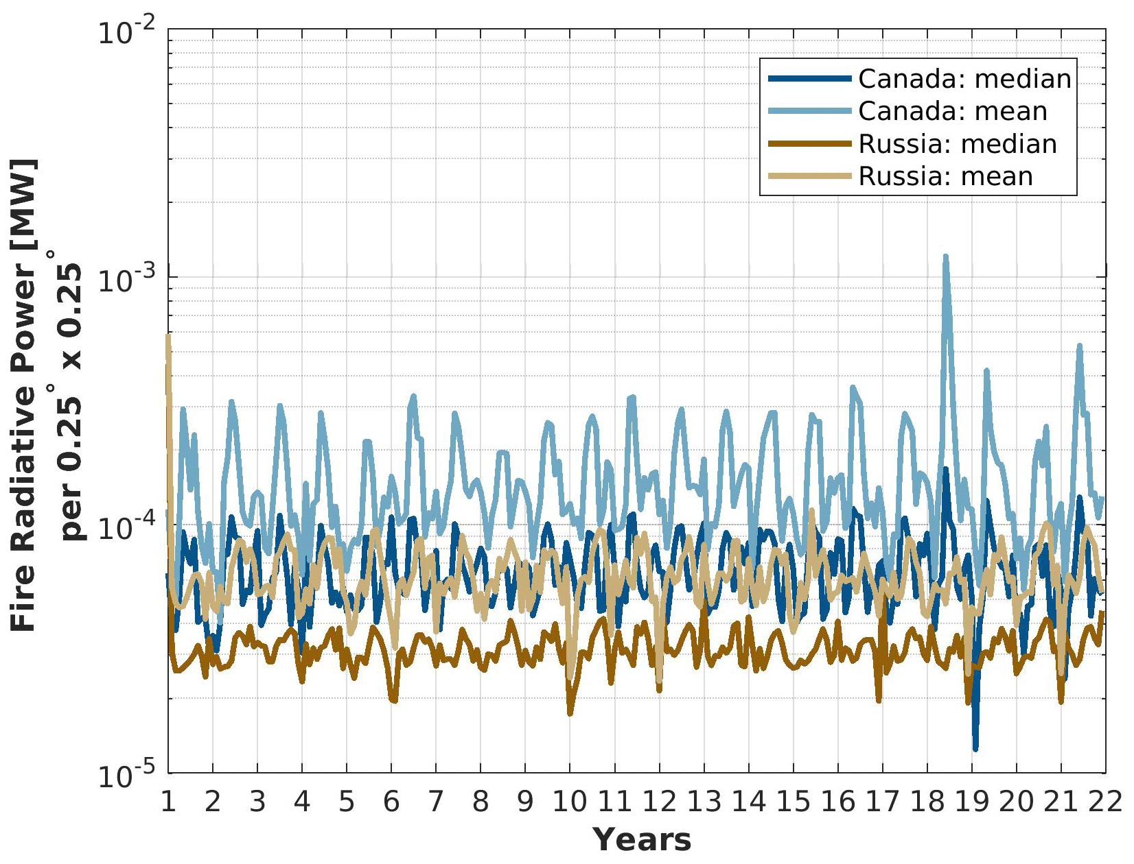
Figure 3 Overview of monthly averaged fire radiative power (FRP) over the entire domain of either “Canada” or “Russia” from 2001–2022.

The wildfire season is in general more pronounced in Canada than in Russia throughout the year after averaging over the entire domain, since the variability from year to year is larger. It can be seen that the observed fire radiative power per grid cell does not increase during the observed 21 years, neither for Russia nor for Canada. The year 2021, which is selected for this study, shows a slightly higher FRP than other years in “Canada” but not in “Russia”. Generally, strong biomass burnings produce clearly visible aerosol layers in lidar observations, which are visible at least for several weeks (e.g., Zielinski et al., 2020; Ohneiser et al., 2021; Cheremisin et al., 2022). Since the aerosol layers from biomass burnings can reach altitudes of 20 km and more (Ohneiser et al., 2023), they would also influence our lidar observations. We have not found such layers in our data set of 2021. Nevertheless the possibility must be considered that aerosol from biomass burning events leads to a higher stratospheric background in the Arctic in summer and autumn. We therefore conclude that biomass burnings did not play a major role in the stratospheric aerosol budget in 2021.

3.2 Tropopause calculations

The tropopause is a transport barrier between the troposphere and the stratosphere. We used the daily launched radiosonde from AWIPEV as well as ERA5 reanalysis data with a hourly global resolution of 0.3°×0.3° to determine the tropopause height for every lidar profile. A full description of the two data sets are given by Maturilli and Kayser (2017) and Hoffmann and Spang (2021), respectively. As the definition of the tropopause, the lapse rate definition, $\frac{\mathrm{d}T}{\mathrm{d}z}\le \mathrm{2}$ K km⁻¹, of the World Meteorology Organisation (WMO; World Meteorological Organization, 1957) is used for both data sets.

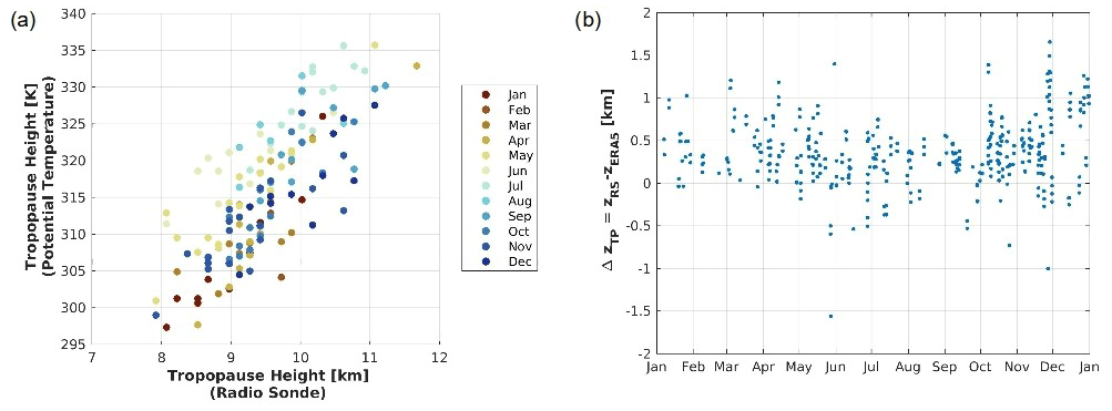
Figure 4 Annual cycle of tropopause (TP) height measured by radiosondes in relation to the potential height of the tropopause derived from radiosondes (a). The deviation between radiosonde tropopause height and ERA5 data is given in [km] (b).

The tropopause height is shown in Fig. 4. Since the measurements of radiosonde and lidar are based on the geometric height, we transformed the altitude into potential temperature for better comparison with CLaMS results, which is based on isentropic coordinates in the stratosphere. Figure 4a shows the geometric height in [km] and compares it with the corresponding potential temperature at this point, θ:

$$\begin{array}{}\text{(5)}& \mathit{\theta }=T{\left({\displaystyle \frac{p_{\mathrm{0}}}{p}}\right)}^{\frac{R}{c_p}}.\end{array}$$

Here T and p are the current temperature [K] and pressure [hPa] of the air parcel, respectively; p₀=1013 hPa the ground reference pressure; R the gas constant of air; and c_p the specific heat capacity. We set $\frac{R}{c_p}=\mathrm{0.286}$.

Every data point in Fig. 4a corresponds to a measurement day. For comparison we also calculated the geometric tropopause with ERA5 data and compared them with radiosonde data throughout 2021 (Fig. 4b). Since there is only one radiosonde launch a day, the lidar measurement time and the launch does not always match, but the deviation between both measurements is maximum 12 h. On the other hand the data by Hoffmann and Spang (2021) have an hourly resolution corresponding to the chosen lidar resolution. The median tropopause height in the radiosonde data is at 314.5 K (9011 m) and on average 329 m above the results of the ERA5 reanalysis model.

It can be seen that in general the tropopause has a higher potential temperature in summer than in winter, but there is also a variability within a month. We conclude nevertheless that the tropopause is always at θ<340 K and aerosol above it is always in the stratosphere with increasing geometric height during summer months. Generally, the annual cycle of the tropopause observed by radiosondes is well represented in the ERA5 data.

3.3 Observations by KARL

In the following study we concentrate on the year 2021, since we have qualitatively good lidar measurements throughout the entire year as well as every month with 481 h for 532 nm and 474 h for 355 nm. Due to additional campaign activity, especially in November and December, and due to high cloud cover fraction, especially in summer (Graßl et al., 2022), the absolute number of measurement time varies a lot between months and seasons. February has the smallest amount of good data at 3 h, while in November 103 h of measurements is available. An overview of the monthly measurement time [h] is given in Table 2. Since the quality checks are performed for each emitted wavelength independently, a deviation in the available amount of measurement time might occur.

Table 2 Overview of the available monthly measurement times [h] for 355 and 532 nm after quality check.

Figure 5 shows the monthly medians of two aerosol backscatter coefficients β₅₃₂ and β₃₅₅ for the selected four heights of the lower stratosphere with a thickness of 20 K, which corresponds to about nine vertical measurement points with the given resolution.

Figure 5 Monthly median backscatter values for β₅₃₂ (green colors) and β₃₅₅ (blue colors) for the lower stratosphere (330 to 410 K potential temperature).

Generally, a weak annual cycle with minimal values of backscatter in spring and highest values in autumn can be seen. However, the curves are quite smooth, especially for 532 nm. At 400 K the amplitude of the annual variability is around 27 % and 25 % for 355 and 532 nm, respectively.

For all four selected layers β₃₅₅ is always larger than β₅₃₂. Further, the backscatter decreases noticeably with increasing potential temperature. While the annual cycle of the backscatter in the lower two altitude ranges seems to be more variable and “disturbed”, with a secondary maximum already in April or May. Between 370 and 410 K, an increase in both backscatter coefficients is found from June to October 2021. As the backscatter and the amplitude of the annual cycle is larger in the UV we conclude that these changes refer to smaller particles, since the scattering efficiency strongly depends on the particle radius (Mie, 1908). The estimation of the effective radius of stratospheric aerosol by Mie calculations will follow in Sect. 3.4. Exemplary days will be later discussed and linked to CLaMS simulations in Sect. 3.5.

3.3.1 Color ratio

The color ratio, CR, is a crucial parameter to determine the size of aerosols and is defined according to Eq. (3). An overview of the CR in 2021 is shown in Fig. 6. As a ratio of two small quantities, CR critically depends on noise and numerical assumptions in the lidar evaluation (Foken, 2021). Hence, some noise is noticeable in the form of rapidly changing colored dots in Fig. 6.

Figure 6 Overview of the color ratio, CR, throughout 2021.

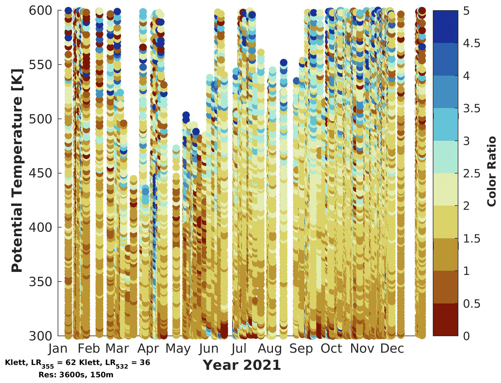
Typically, CR values around 2 have been found. Remarkable is the fact that the second half of the year becomes more homogeneous with slightly larger values than the first half. From June to October a more homogeneous distribution of a CR∼2 is detected between 320 and 440 K potential temperature. Since CR is a function of particle radius, the particle size decreases towards the end of the year and additionally with increasing height, as was also seen by Junge et al. (1961a). According to Murphy et al. (2021) the generally larger particles (lower CR) in the first half of the year may be an indication of reduced tropospheric advection in the Arctic lower stratosphere in this time of year.

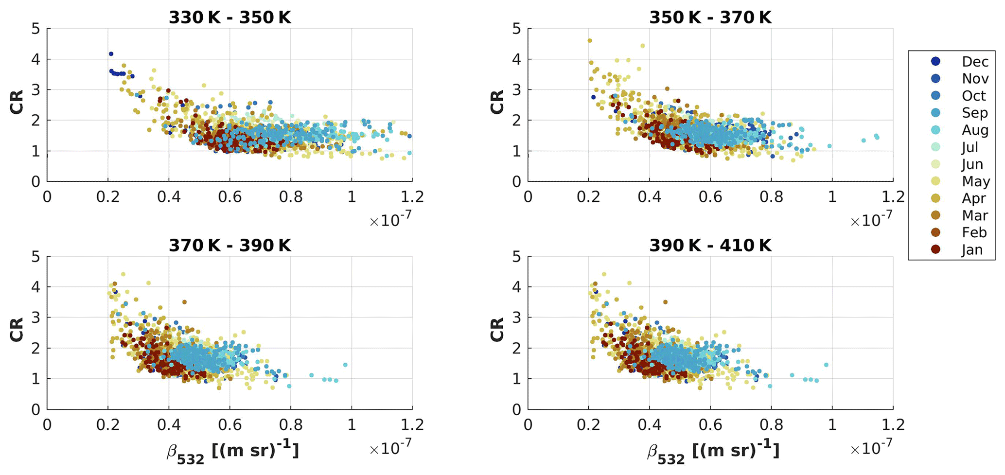
Figure 7 Dependency of CR and β₅₃₂ for four selected height intervals of the lower stratosphere.

The relationship between β₅₃₂ and CR is depicted for the previously defined four layers of the lower stratosphere in Fig. 7. With this dependency a better understanding of the particle size and concentration can be made.

While the spread in β₅₃₂ decreases with height, CR remains in this same range of about $\mathrm{CR}\in [\mathrm{1},\mathrm{4}]$. At altitudes of 330–350 K a small influence of the troposphere might be seen in summer months, since the tropopause can reach these altitudes exceptionally. In the range of $\mathrm{CR}\in [\mathrm{1},\mathrm{2}]$ all altitude layers have a backscatter coefficient larger at the end of the year than in the beginning. Under pristine conditions, ${\mathit{\beta }}_{\mathrm{532}}\le \mathrm{5}\times {\mathrm{10}}^{-\mathrm{8}}$ (m sr)⁻¹, we see always a clear dependence between CR and β: the smaller β (the clearer the atmosphere) becomes, the larger CR becomes because small particles show only a small scattering efficiency. Hence, below ${\mathit{\beta }}_{\mathrm{532}}=\mathrm{5}\times {\mathrm{10}}^{-\mathrm{8}}$ (m sr)⁻¹ the stratospheric β is mainly driven by the size of aerosols. This effect levels to above the limit of ${\mathit{\beta }}_{\mathrm{532}}=\mathrm{5}\times {\mathrm{10}}^{-\mathrm{8}}$ (m sr)⁻¹. After a certain limit the stratospheric aerosol does not grow apparently. This is in agreement with the annual cycle already shown in Fig. 5. Since the color ratio does not change much in the four discussed intervals, it also means the aerosol size is very similar, but only the concentration becomes lower the higher up the layer is located.

3.3.2 Aerosol depolarization

Another parameter to determine physical properties of aerosol by remote sensing is using the so-called aerosol depolarization, δ^aer(λ). It is defined according to Eq. (3). The laser of KARL is linearly polarized and is always the reference direction of the scattered light. With Mie theory it can be shown that spherical particles do not change the polarization of the laser light, while non-spherical ones do. Due to surface tension liquid droplets are in general spherical (Foken, 2021).

In general stratospheric aerosols have the property of ${\mathit{\beta }}_{⟂}^{\mathrm{aer}}\ll {\mathit{\beta }}_{\parallel }^{\mathrm{aer}}$. Therefore, it is expected that δ^aer becomes quite noisy for a standard aerosol measurement at higher altitudes. Due to generally low values of the depolarization we only show and discuss δ₅₃₂ in this study.

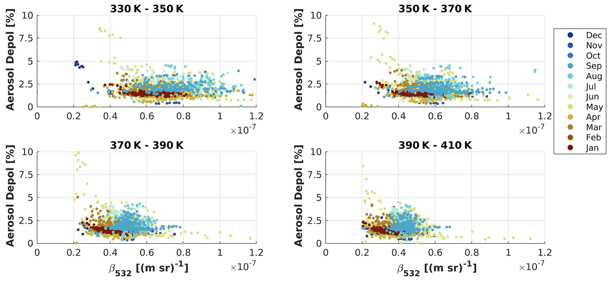
Figure 8 Dependency of β₅₃₂ and δ₅₃₂ for the four selected altitudes in the lower stratosphere.

The overview of the aerosol depolarization, δ₅₃₂, is given in Fig. 8 for the different layers of the lower stratosphere color-coded for every month. Due to case studies in Sect. 3.5 September is highlighted here already. The depolarization is low (< 10 %) for all corresponding values of β₅₃₂. All four height intervals a common depolarization is between δ₅₃₂≥1 % and δ₅₃₂≤4 %. Additionally May is the most diverse month with single cases of δ₅₃₂→10 %, while January shows the smallest depolarization. In general, summer has a higher depolarization than winter months.

Table 3 Relative occurrence of at least a “weak” polarization (δ₅₃₂=2 %–5 %) in different altitude layers of the lower stratosphere. All numbers are given in [%]. The low numbers in February can also be explained by the low number of measurement points (see Table 2).

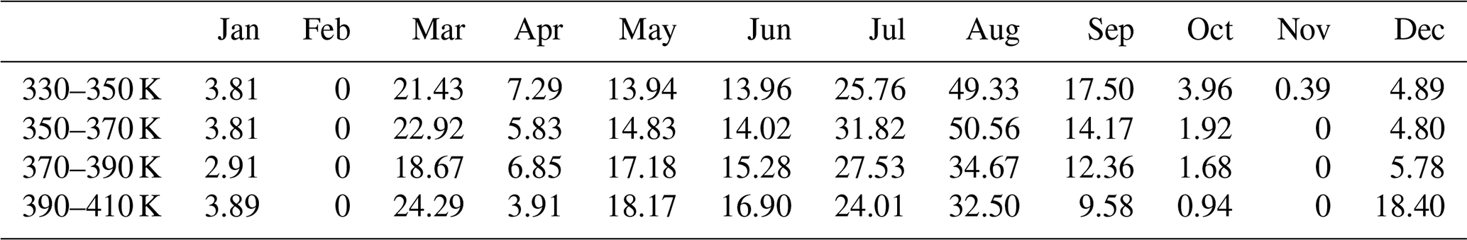
Table 4 Relative occurrence of at least a “medium” polarization (δ₅₃₂=5 %–10 %) in the lower stratosphere from 330–410 K. The numbers are given in [%].

We define a “weak” depolarization with δ₅₃₂=2 %–5 % (see Table 3), a “medium” depolarization with δ₅₃₂=5 %–10 % (see Table 4) and a “strong” depolarization with δ₅₃₂≥10 %, but this was not found in the lower stratosphere of 2021.

A big variability between the months can be observed in Table 3 for the depolarization of δ₅₃₂=2 %–5 %. While the depolarization is in general lower in the winter months, it reaches its maximum in August and has a clear annual cycle. The depolarization never reached values > 2 %. This indicates that the stratospheric aerosol observed above Ny-Ålesund is not constant throughout the year but changes its chemical composition and/or its shape (Foken, 2021). Furthermore, a more frequent depolarization is found at lower altitudes than at higher ones. Our lidar observations fit very well with the physical properties of aerosols in the Asian tropopause aerosol layer (ATAL), which consist of organics, nitrate, sulfate and ammonium, especially in combination with Fig. 8, where it can be seen that the aerosol is also slightly non-spherical (Appel et al., 2022). The altitude at which this aerosol layer in the Arctic was found also matches very well with the altitude of the ATAL.

Table 4 shows on the other hand the relative occurrence of δ₅₃₂=5 %–10 % for the entire layer of 330–410 K. Only in a few months was a “medium” depolarization observed. Even though the depolarization has an annual cycle, all values are very small compared to lower latitudes (Foken, 2021). No young extreme pollution events, like wildfire aerosol, dust intrusion or volcanic ash with typical values of δ₅₃₂≥16 % (Foken, 2021), were found in the lidar measurements over Ny-Ålesund in 2021. Therefore we conclude that our data set indeed mainly represents stratospheric background conditions even with the contribution of the ATAL. Therefore we conclude that our data set represents stratospheric conditions free from the influence of local events; however there is evidence of a seasonal impact of ATAL particles on the lower stratosphere during summer.

Figure 9 shows the two months with the lowest (February) and highest median depolarization (August) for comparison for the lower stratosphere and for further investigating the difference between the relative occurrence of depolarization.

Figure 9 Mean aerosol depolarization, δ₅₃₂, for the two exemplary months of February and August. The grey shaded area shows the difference between both months.

While February has a more or less constant depolarization at δ₅₃₂=1.35 % in the atmosphere between 320 and 480 K, August on the other hand has in general higher depolarization values, especially in the lower parts of the atmosphere (until about 420 K). The grey shaded area highlights the difference between both months. Especially in the troposphere and lower stratosphere a significant deviation can be found and shows the impact of the ATAL. Additionally, the summer month also has a maximum around 315 K, where it reaches δ₅₃₂=2.5 %, followed by a second, local maximum at around 340 K with δ₅₃₂=2.0 %. From that point on it decreases to about δ₅₃₂=1.25 % and converges to the same value as in February. Due to solar radiation in August, the data become noisy quicker than during polar night. At an altitude of 400 K the depolarization in August is still significantly higher than in February. The median tropopause height according to radiosonde data is 307 K in February, while it is 324 K in August. This plot also shows that even if no distinct biomass burning layer has been seen in our lidar data during summer, the slightly less spherical shape of the particles indicates a non-sulfuric component that is an evidence for an impact of ATAL particles on the Arctic background aerosol up to ∼ 450 K in August 2021, even though aged biomass burning aerosol may still contribute to the stratospheric aerosol background, which was even found at altitudes of up to 27 km (Ohneiser et al., 2023).

3.3.3 Seasonal variability in stratospheric Arctic background aerosol

Our measurements indicate evidence for the impact of ATAL particles on the Arctic stratosphere during summer; therefore we now present the annual cycle of β₃₅₅ and β₅₃₂ of the background aerosol in Figs. 10 and 11, respectively, for two different heights of 360 and 380 K. Data from ±10 K around the chosen level are taken into account for the following study.

Figure 10 Annual cycle of stratospheric aerosol backscatter coefficient β₃₅₅ at 360 and 380 K height. The red − and + symbols show median and average, respectively. The blue boxes symbolize the 25th and 75th percentiles. The black lines show accordingly the 9th and 91th percentiles.

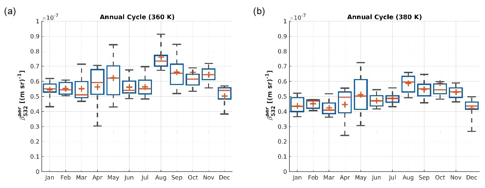
Figure 11 Annual cycle of stratospheric aerosol backscatter coefficient β₅₃₂ at 360 and 380 K height. The red − and + symbols show median and average, respectively. The blue boxes symbolize the 25th and 75th percentiles. The black lines show accordingly the 9th and 91th percentiles.

The annual cycle of β₃₅₅ at 360 K altitude (Fig. 10a) shows a small seasonal dependency: while the first half of the year is characterized by lower values of the backscatter coefficient, the mean values of August, September and November are $>{\mathrm{10}}^{-\mathrm{7}}$ (m sr)⁻¹. While winter (DJF) is the clearest season, May, July and September are the months with the broadest distribution. Overall the median and mean values are for all months very similar, indicating that β₃₅₅ follows almost a Gaussian distribution.

Likewise there is a similar annual cycle in the data at the 380 K level (Fig. 10b) with larger values from June to November. Also here DJF is the clearest season. While the absolute values of β₃₅₅ are consistently lower than at 360 K height, the relative spreading of β₃₅₅ is also smaller. Typical values for 360 K altitude are ${\mathit{\beta }}_{\mathrm{355}}\in [\mathrm{7},\mathrm{11}]\times {\mathrm{10}}^{-\mathrm{8}}$ (m sr)⁻¹, and they are smaller for the 380 K level, ${\mathit{\beta }}_{\mathrm{355}}\in [\mathrm{6},\mathrm{10}]\times {\mathrm{10}}^{-\mathrm{8}}$ (m sr)⁻¹. In summary, a clear annual cycle in the stratospheric backscatter coefficient has been found.

While the values of β₅₃₂ are by about a factor of 1.5 to 2 smaller than for β₃₅₅, a similar pattern is shown in Fig. 11a compared to β₃₅₅ with some differences: the variability in the first half of the year is more pronounced, and the increased backscatter coefficient peaks in August. On the other hand β₅₃₂ is less homogeneously distributed than β₃₅₅ throughout the entire year. The 380 K level (Fig. 11b) shows the same trend throughout the year with a higher month-to-month variability in April and May. Median and mean values of β₅₃₂ spread more than for β₃₅₅, indicating a more asymmetrical distribution and more variability within a month. Typical values for 360 K altitude are ${\mathit{\beta }}_{\mathrm{532}}\in [\mathrm{5},\mathrm{7}]\times {\mathrm{10}}^{-\mathrm{8}}$ (m sr)⁻¹ and for the 380 K level ${\mathit{\beta }}_{\mathrm{532}}\in [\mathrm{1},\mathrm{6}]\times {\mathrm{10}}^{-\mathrm{8}}$ (m sr)⁻¹.

3.4 Mie calculus for particle size estimations

Absorption and scattering of a single spherical particle surrounded by a non-absorbing medium are described by Mie scattering (Mie, 1908). Particles can have a complex refraction index, m, in general:

$$\begin{array}{}\text{(6)}& m=n+ik,\end{array}$$

where ℜ(m)=n describes the scattering and ℑ(m)=k the absorption of the light by aerosols. The scattering efficiency factor is a parameter which is defined as the ratio of the scattering cross section, σ_eff (Eq. 7), to the geometrical cross section. Therefore, it is a good measure to determine the effective radius, r_eff, for a mono-modal log-normal aerosol size distribution:

$$\begin{array}{}\text{(7)}& {\mathit{\sigma }}_{\mathrm{eff}}=\mathit{\pi }\underset{\mathrm{0}}{\overset{\mathrm{\infty }}{\int }}{Q}_{\mathrm{sca}}^{\mathrm{FF}}\left(r_{\mathrm{eff}}\right)r^{\mathrm{2}}{f}_{\mathrm{1}}\left(r_{\mathrm{eff}}\right)\mathrm{d}{r}_{\mathrm{eff}}.\end{array}$$

The scattering efficiency $Q_{\mathrm{sca}}^{\mathrm{FF}}\left(r_{\mathrm{eff}}\right)$ for the far field, FF, and f₁ the mono-modal log-normal aerosol size distribution follow the calculations according to Bohren et al. (2023).

We expect small or already aged aerosols in the stratosphere (Turco et al., 1982; Kremser et al., 2016) and are therefore able to estimate the effective radius of these particles through the Library for Radiative Transfer – libRadtran (http://libradtran.org/doku.php, last access: 13 June 2024) (Mayer and Kylling, 2005; Emde et al., 2016). As Kremser et al. (2016) pointed out, sulfur chemistry is a very common and frequent process in the stratosphere. Since sulfate-containing particles are not the only aerosol type in the ATAL, we also chose biomass burning particles as the second example as a highly absorbing particle type.

We roughly estimate an effective radius for the observed aerosol, which can have a lifetime of up to several weeks (Oppenheimer et al., 1998). Since the refractive index is wavelength-dependent, two different indices were chosen for sulfate: $m_{\mathrm{532}}^{\mathrm{Sulfate}}=\mathrm{1.44}+{\mathrm{10}}^{-\mathrm{4}}i$ (Russell and Hamill, 1984; Yue et al., 1994) and $m_{\mathrm{355}}^{\mathrm{Sulfate}}=\mathrm{1.41}+\mathrm{0}i$. The imaginary part of Eq. (6) can be neglected for $m_{\mathrm{355}}^{\mathrm{Sulfate}}$, since sulfate does not absorb in UV (Beyer and Ebeling, 1998; Washenfelder et al., 2013). As a comparison we also calculated the effective radii for a strongly absorbing aerosol type, like from wildfires, and chose a refractive index of biomass burning (BB) aerosols of $m^{\mathrm{BB}}=\mathrm{1.52}+{\mathrm{10}}^{-\mathrm{2}}i$ for 355 and 532 nm (Sumlin et al., 2018).

With the above-mentioned assumptions we used the two refractive indices for 355 and 532 nm, a log-normal distribution of particles with a standard deviation of σ=1.5 up to a maximum size of 600 nm, and a bin with of the distribution of 10 nm.

As Fig. 12 shows, the larger the real part of the refractive index is, the quicker the scattering efficiency drops for larger effective radii. Simultaneously the maximum of scattering efficiency moves towards larger r_eff for larger real parts and wavelengths. On the other hand, there is not a big difference in scattering efficiency for large particles, especially for biomass burning aerosol observed at the wavelengths of 355 and 532 nm, even though the efficiency is much lower for smaller particles at 532 nm. An overview of the different effective radii correlated to typical color ratios (see Sect. 3.3.1) is given in Table 5.

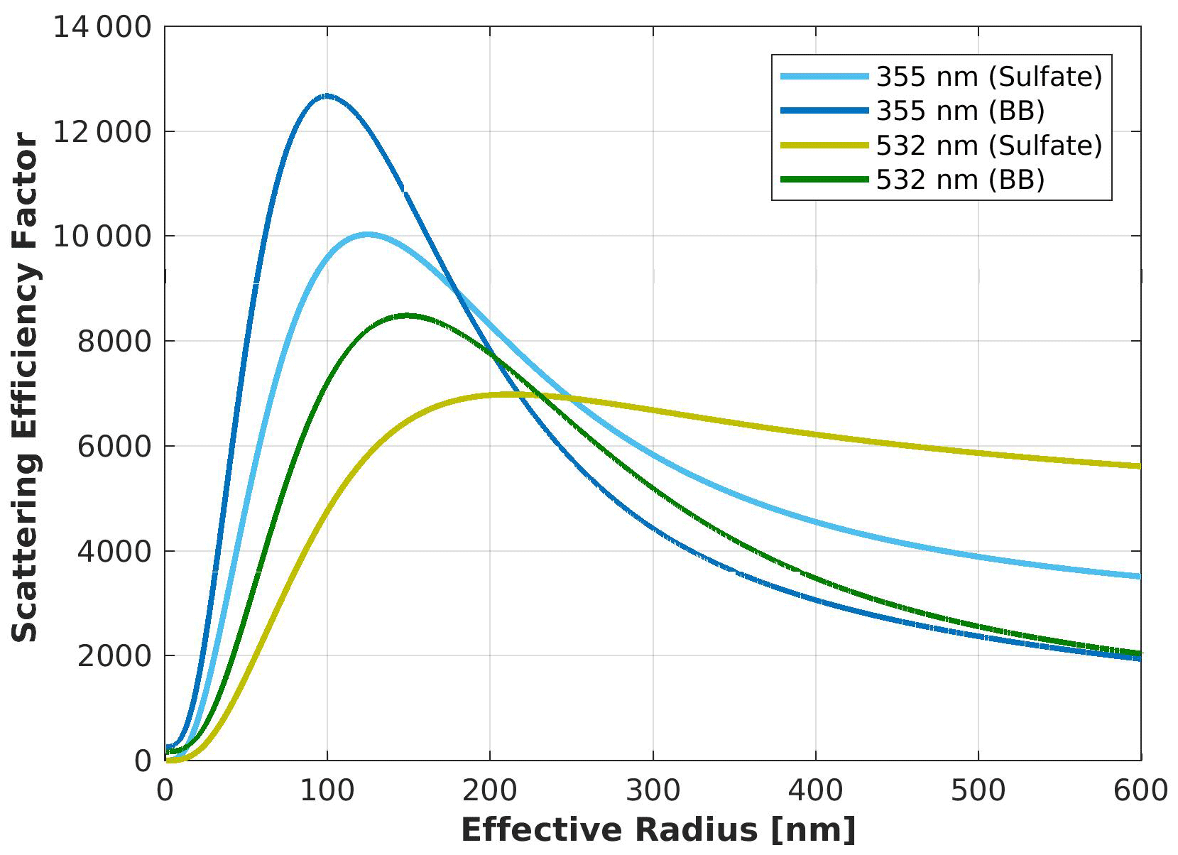
Figure 12 Scattering efficiency factor, $Q_{\mathrm{sca}}^{\mathrm{FF}}$, in arbitrary units for the emitted 355 and 532 nm laser beam for a log-normal distribution of purely sulfate particles and strongly absorbing BB aerosols.

Table 5 Calculated effective radii, r_eff [nm], corresponding to typical color ratios with $m^{\mathrm{BB}}=\mathrm{1.52}+{\mathrm{10}}^{-\mathrm{2}}i$, $m_{\mathrm{532}}^{\mathrm{Sulfate}}=\mathrm{1.44}+{\mathrm{10}}^{-\mathrm{4}}i$ and $m_{\mathrm{355}}^{\mathrm{Sulfate}}=\mathrm{1.41}+\mathrm{0}i$.

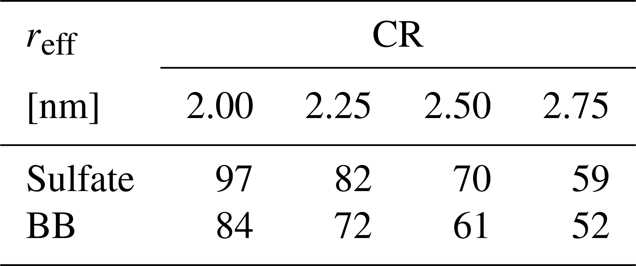
It is expected to find a small effective radius for stratospheric aerosol distributions, since the particles form in chemical reactions in Aitken mode on salt solutions or salt embryos. The reaction takes also place at stratospheric temperatures of $T\le -\mathrm{55}$ °C (Friend et al., 1973). With these small effective radii corresponding to a height-dependent value of CR (see Fig. 6) we conclude that in general the effective radius of aerosol in the lower stratosphere is relatively small (Murphy et al., 2021) and the particles are sorted according to their size by for example sedimentation processes with an accumulation of largest particles close to the tropopause.

3.5 Origin of air masses inferred from CLaMS simulations

Backscatter coefficients, color ratio and depolarization of the aerosol particles detected by KARL show evidence that the ATAL has an impact on the Arctic lower stratosphere. To confirm this assumption we link KARL measurements to Lagrangian transport simulations. To identify the source regions of the aerosols detected by KARL, global three-dimensional CLaMS simulations including surface origin tracers were analyzed and discussed for two exemplary days in September 2021 (13 and 28 September). The identification of possible source regions of the aerosol particles found above Ny-Ålesund (Sect. 3.5.1) is investigated by global three-dimensional CLaMS simulations including surface origin tracers (Sect. 3.5.2) as well as CLaMS back trajectories (Sect. 3.5.3).

3.5.1 Seasonal variability in air mass origins over Ny-Ålesund

The contributions of young air masses from South Asia and the tropical Pacific over the course of the year 2021 to the air over Ny-Ålesund is inferred for the heights (360±5) K (Fig. 13a) and (380±5) K (Fig. 13b), respectively. Mean values are calculated for the surface origin tracers for each day.

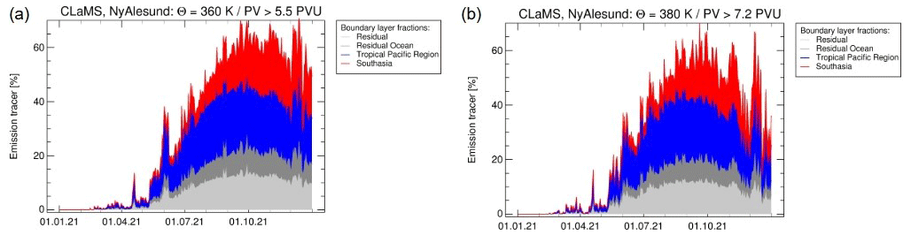
Figure 13 Contribution of different surface emission tracers from South Asia, tropical Pacific region, residual and residual ocean to the lower stratosphere above Ny-Ålesund at 360 K (a) and 380 K (b) potential temperature for the year 2021. The 5.5 and 7.2 PVU surface takes the climatological isentropic transport barrier at 360 and 380 K, respectively, into account (Kunz et al., 2015).

Artificial tracers released in the model simulations since 1 December 2020 in Fig. 13 do not reach Ny-Ålesund at levels of potential temperature of 360 and 380 K before May 2021. During summer and autumn, the highest fractions of tropospheric air over Ny-Ålesund are from South Asia and the tropical Pacific region. Especially in September and October almost 20 % of the air is from South Asia. These model results support the evidence that the Arctic lower stratosphere is impacted by aerosol particles from the ATAL (Yu et al., 2017; Bian et al., 2020). All other regions combined are of minor importance. With few exceptions the tropical Pacific region contributes constantly more, and sudden changes in its impact are rare.

The accumulation of young air masses in the lower stratosphere over Ny-Ålesund is lower than 100 % during the year 2021. The remaining fraction consists of aged air that is older than 1 December 2020 when the CLaMS simulation was initialized.

3.5.2 Three-dimensional CLaMS simulation

Figure 14 gives for two exemplary days in September (13 and 28 September) the distribution of the surface origin tracer for South Asia (a marker for air from the Asian monsoon region) over northern Europe at 360 and 380 K potential temperature. A high fraction from South Asia is found over the Arabian Peninsula marking the western outflow of the Asian monsoon anticyclone (e.g., Vogel et al., 2016). Air masses contributing to the ATAL can be transported eastwards along the subtropical jet and enter the lower stratosphere by quasi-horizontal transport. As a result, thin filaments with enhanced signatures of air mass tracers originating from South Asia were found over the northern Atlantic Ocean and Europe (e.g., Vogel et al., 2016; Wetzel et al., 2021; Lauther et al., 2022). On 28 September a filament located over Ny-Ålesund with a contribution from South Asia up to 40 % is simulated. This filament was not found on 13 September.

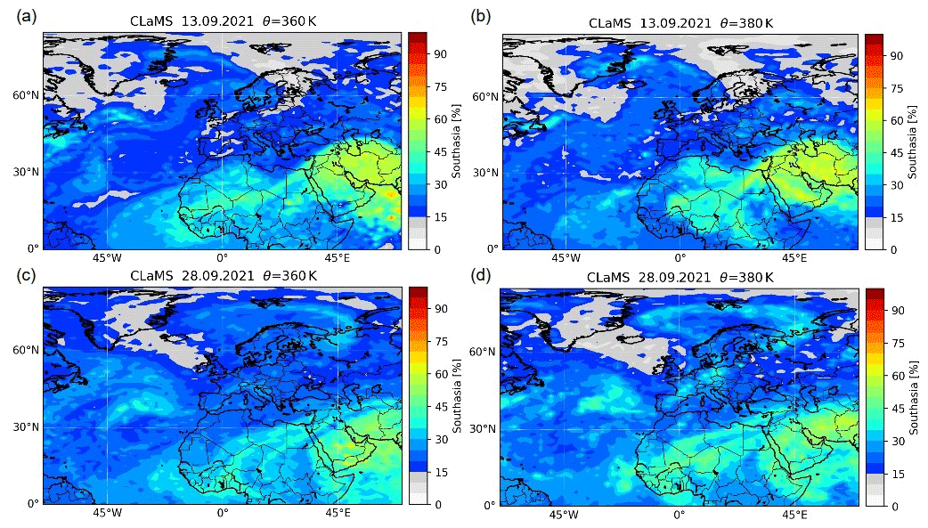
Figure 14 Horizontal distribution of the fraction of air originating in South Asia (details of the region can be found in Fig. 2) at 360 K (a, c) and 380 K (b, d) potential temperature on 13 September (a, b) and 28 September (c, d) 2021.

Figure 14 shows the impact of Southeast Asia on the stratosphere for the two different heights of 360 and 380 K. On 13 September the contribution is quite low at 360 and 380 K (Fig. 14a and b). As can be seen in both figures, the contribution is constant over the whole of Europe but increases with increasing height and changes on timescales of less than a day. As can be seen at both altitudes, the impact is already very low over Svalbard (≈ 10 %). On 28 September a filament was seen faint at 360 K altitude (Fig. 14c) but very pronounced at 380 K (Fig. 14d). The presented values of 20 % above Ny-Ålesund are large for the site but small compared to locations at lower latitudes.

When comparing Figs. 13 and 14 with each other the contributions of the two main sources of tracers can be identified. The region “tropical Pacific” is responsible more for the background amount, which can be observed in Fig. 14. Contrary to this, “Asia” has a smaller contribution but shows also a very large day-to-day variability. These spikes can be nicely seen as filaments in the three-dimensional simulations of tracers of Fig. 14.

The following preliminary conclusion can be made: there is a large day-to-day variability in the distribution of young air masses from Asia contributing to the Arctic lower stratosphere. This variability strongly depends on the dynamics of the Asian monsoon anticyclone itself and the transport of air masses from Asia to the extratropical lower stratosphere.

3.5.3 Case studies using back-trajectory calculations

Backward trajectories are well suited to analyze the detailed transport pathway of an air parcel and therefore complement the three-dimensional CLaMS simulations (e.g., Vogel et al., 2014; Wetzel et al., 2021; Lauther et al., 2022). Within this study, we calculated an ensemble of backward trajectories for the two exemplary days (13 and 28 September 2021). Within ±2° in latitudinal and longitudinal direction around Ny-Ålesund and in a height range of 360 to 380 K, 891 trajectories have been calculated in total for each day. Markers in Fig. 15 show the location where the trajectory first reaches the boundary layer. The color indicates the transport time.

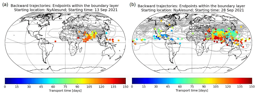
Figure 15 Location of trajectory endpoints where they reach the model boundary layer (BL). Trajectories are initialized on 13 and 28 September within 360 and 380 K in altitude and ±2° horizontally around Ny-Ålesund. The endpoints are color-coded by the transport time between reaching the boundary layer the first time and the lidar measurement at Ny-Ålesund.

As can be seen in Fig. 15a, on 13 September in total 41 trajectories (4.6 %) reached the boundary layer in Southeast Asia after traveling for about 3 to 4 months, and 6 other trajectories (0.7 %) are outside of the monsoon region. A total of 850 trajectories (89.6 %) did not touch the boundary layer at all within the model run time.

The situation is a bit different for 28 September 2021 (Fig. 15b), where the fraction of contacts outside of the monsoon region is larger (6.1 %) but also the fraction of endpoints in Southeast Asia (17.8 %​​​​​​​). On this day 76.1 % of the 891 trajectories did not reach the model boundary layer within the computational time. It took the air parcel on average 87 d to reach Ny-Ålesund on 28 September. As can be seen on both days, back trajectories also end in different parts of the world, like the equatorial Pacific Ocean but also Central America. This result agrees very well with the forward trajectories of aerosol tracers of Sect. 3.5.2. The average transportation time from the Asian summer region to Ny-Ålesund is about 1 month longer on 13 September (111 d) than on 28 September (87 d).

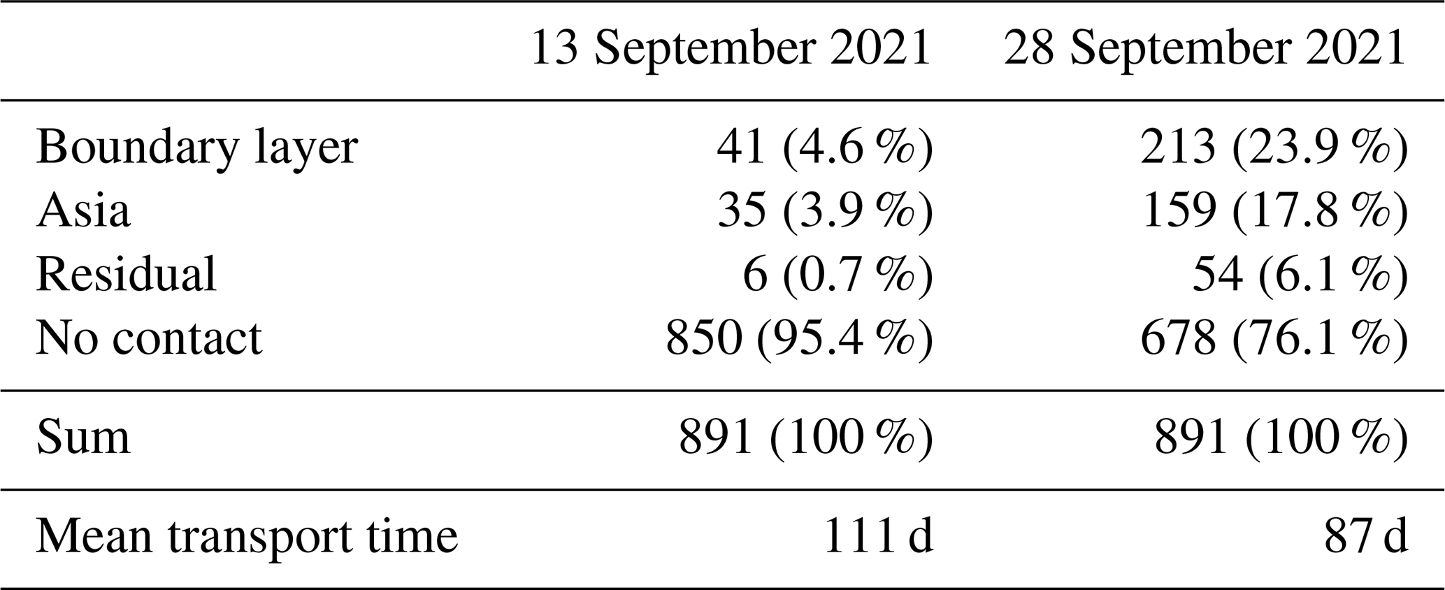
The presented numbers are also given in Table 6 for a better overview, with the absolute and relative numbers of back trajectories touching the boundary layer inside and outside of the monsoon region in South Asia.

Table 6 Contact points of all calculated back trajectories, which are presented in Fig. 15 with their relative and absolute frequencies as well as the mean propagation time between the Asian summer monsoon region and Ny-Ålesund.

Additionally one trajectory ensemble is given for each day in Fig. 15. As can be seen in both cases, the artificial tracer circulates from Ny-Ålesund first around the pole before it moves to lower latitudes until it reaches South Asia, where it also circles until it reaches the boundary layer. Since both trajectories have similar pathways, we conclude that the intake of aerosols into the lower stratosphere depends on the local conditions in South Asia and the effectivity for aerosols being lifted into the ATAL.

3.6 Detailed analysis with KARL

In the following these two exemplary days will be discussed in detail. On one of them CLaMS observed a filament in different heights. The other day is an example with a comparable clear stratosphere. As a reference day a profile of February was additionally plotted to emphasize the difference between seasons and days. Here the backscatter ratio, defined according to Eq. (4), is used as it does not decrease with increasing height and layers are easier to detect.

Figure 16 Profiles of different parameters – R₅₃₂ (a), δ₅₃₂ (b) and CR (c) – for the two exemplary days. The date 28 September is shown here twice, since the lidar measurement simultaneously took place with the model output at 12:00 UT. As a comparison the lidar results are also shown at 16:00 UT for 28 September. The shaded area highlights the difference between February and the filament on 28 September.

Figure 16 shows R₅₃₂ (Fig. 16a), δ₅₃₂ (Fig. 16b) and CR (Fig. 16c) for the two exemplary days in September with and without a detected filament by CLaMS. The shaded area highlights the difference between a typical profile of February, which is also not affected by the ATAL, and the detection of the filament on 28 September at 12:00 UT. Since the model output of CLaMS is shown in Fig. 14 for 12:00 UT and the size and movement of the filaments indicate only a short temporal increasing of the backscatter ratio, the measurements by KARL on 28 September are shown twice: for 12:00 and 16:00 UT. Due to the horizontal transports in the stratosphere the filament of this day has already moved out of the line of sight of the lidar for the later time. According to the radiosonde data, the tropopause is well defined on 28 September 2021 at 332.9 K. The reanalysis data of tropopause heights from the data repository Jülich DATA (Hoffmann and Spang, 2021) reveal a tropopause height of 329.1 to 335.1 K over Ny-Ålesund for the two lidar profiles. For this case the air masses of troposphere and stratosphere are well separated from each other, and an exchange is not possible.

Generally, it can be seen that all parameters, backscatter ratios, aerosol depolarization values and color ratios are larger and less variable for all days in September than in February, as was already shown in Figs. 10 and 11. This implies that the stratospheric aerosol is already aged and well-mixed.

The backscatter ratio reveals a layer on 28 September at 12:00 UT between 360 and 400 K. This one is also seen in CLaMS as filaments (Fig. 14c and d). KARL and CLaMS also agree that the layer is more pronounced at 380 K than at 360 K. According to KARL the layer reaches until 400 K altitude. Compared to 12:00 UT the layer at 16:00 UT has already a significantly decreased backscatter ratio, which is almost at the background level (defined as the mean backscatter ratio of the measurements not affected by the filament). From Fig. 16a it can be seen that the strongest impact of the filament occurred around 390 K. R₅₃₂ rises from about R₅₃₂=1.14 to R₅₃₂=1.165. This corresponds to an increase in aerosol backscatter of about 15 %.

The depolarization is in general quite small with values around 2.5 % at 340 K and a maximum of all profiles at around 360 K. δ decreases with increasing heights to values around 2 % at 420 K. These small values indicate nearly spherical particles throughout the lower stratosphere. A slight increase in depolarization throughout the entire lower stratosphere is found for 12:00 UT on 28 September, when the filament passes above the station.

The same result of small particles can also be found in the color ratio in Fig. 16c. While CR reaches values around 4 at 340 K, it decreases to CR≈2.9 in the altitude range of 370 to 410 K. This means that aerosols are smallest and reach a constant size distribution. The filament of 28 September changes the overall color ratio only in the altitude range of 385 to 395 K by CR≈0.2, meaning that the particle size is slightly smaller in times with a filament. February reveals a comparable low color ratio (larger particles) but also a lower backscatter ratio. We therefore conclude that aerosols are in general larger but less abundant in February than during September. The fluctuations are also larger, which indicates a less effective vertical mixing of the lower-polar-stratospheric air.

Observations by KARL and modeling studies by CLaMS reveal a good agreement between the results. Filaments which were forecasted by CLaMS were found in KARL data. Physical properties of the stratospheric aerosol in the Arctic in September reveal very similar properties as in the ATAL. We can therefore conclude that the filaments above Ny-Ålesund originate from the ATAL. Stratospheric aerosol in other seasons, like February, has different physical properties and can clearly be distinguished from aerosols arriving in September.

4 Discussion

In MODIS data we did not find any hint that 2021 was exceptional in regards to the wildfire season in the Northern Hemisphere. The detailed studies of Canadian wildfires by Haarig et al. (2018) and Baars et al. (2019) reveal an aerosol depolarization of up to δ₅₃₂≤20 % in the stratosphere. An explanation for the deviation of the aerosol depolarization is the very low relative humidity in the stratosphere (Maturilli and Kayser, 2017). Since the aerosol remained there for already some days, it dried out and took on a spherical shape, with which a depolarization of δ₅₃₂≈2 % is expected and was found in our data. A similarly strong exemplary wildfire event, like was analyzed by Ansmann et al. (2018), was not found in our data.

In this work we showed a clear annual cycle of the stratospheric aerosol for the Arctic in the year 2021. In summer and autumn the aerosol backscatter is larger (by about 20 %) than in winter and spring, especially in the UV. At ALOMAR (Arctic Lidar Observatory for Middle Atmosphere Research, northern Norway) a study about stratospheric aerosols was performed by Langenbach et al. (2019) for the years 2014–2017. The authors found a significantly increased backscatter ratio in the lower stratosphere (12 to 18 km) in the months of July and August for an emitted wavelength of λ=1064 nm. Hence, the Arctic or sub-Arctic stratosphere is not pristine; especially aerosol contamination in summer may be typical. Compared to the stratospheric background aerosol at ALOMAR, we observe the aerosol layer at lower altitudes (in km) and the strongest appearance in August and September. Deviations between these two measurement stations are probably due to the geographical location and the in general lower tropopause height in the Arctic than at lower latitudes.

After aerosol particles or their gas-phase precursors were uplifted into the lower stratosphere by the monsoon system (e.g., Brunamonti et al., 2018; Hanumanthu et al., 2020; Weigel et al., 2021a, b; Appel et al., 2022), the air mass is confined within the Asia monsoon anticyclone from which eddies and filaments can be shed to the east. These polluted air masses are further transported into the stratosphere of the Northern Hemisphere by the breaking of Rossby waves (e.g., Waugh, 1996; Vogel et al., 2016); therefore it is expected to find filaments with an enhanced number of aerosol particles at higher latitudes. Aerosols contributing to the ATAL can circulate a few times around the Asian monsoon anticyclone before leaving Asia. In addition they can be transported along the subtropical jet a few times around the globe until they reach the Arctic. There it can then be further investigated by the lidar KARL by assuming similar propagation velocities as Jumelet et al. (2020). Afterwards the aerosol load decreases slowly by sedimentation and other removal processes happening in the stratosphere described in general by Junge et al. (1961a). From December to July the aerosol load is low and about constant. This is in good agreement with, for example, Junge et al. (1961a) and Kremser et al. (2016), who observed both an equilibrium state of new particle formation out of the gas phase and removal processes from the stratosphere into the troposphere. The physical properties of the filaments in the Arctic stratosphere reveal that the particles originate from the ATAL.

Since various types of aerosols are presented in the ATAL, we estimated the effective radii of two exemplary types: one with purely sulfate-containing particles and the other highly absorbing one from biomass burnings. Mie calculus revealed an effective radius of 52 to 97 nm as two more extreme examples of the aerosol classes. Since the depolarization is comparably small, we also conclude that the predominant aerosol type has a spherical shape, which agrees with the in situ measurements of Junge et al. (1961a), Hofmann et al. (1975), and Murphy et al. (2021) at lower latitudes, and aged aerosols emitted by wildfire events agree with the calculated effective radius of the observed aerosols in the Arctic (120 to 160 nm); this all additionally enhances the assumption of a log-normal particle size distribution (Dahlkötter et al., 2014; Baars et al., 2019).

Taking now the height-dependent calculations of Junge et al. (1961a) into account sedimentation velocities of about $v_{min}=\mathrm{3}\times {\mathrm{10}}^{-\mathrm{3}}$ to $v_{max}=\mathrm{2}\times {\mathrm{10}}^{-\mathrm{2}}$ cm s⁻¹ can be found. Rough estimations of the altitude loss of aerosols due to sedimentation are presented in Table 7, with traveling times of $t_{min}=\mathrm{60}$ d to $t_{max}=\mathrm{120}$ d.

Table 7 Height loss of stratospheric aerosol due to sedimentation while traveling 2 to 4 months from the Asian summer monsoon region to Ny-Ålesund.

Since the fall velocities are so small for these particles, it is probable that they remain long enough in the stratosphere to be transported to the European Arctic. Additionally, due to the slow sedimentation velocity as well as their small size (see Sect. 3.4), aerosol from the monsoon region can reach Ny-Ålesund.

According to CLaMS back-trajectory calculations for the two exemplary days (13 and 28 September 2021) air parcels from surface sources in Asia have transport times from about 2 to 4 months until they reach the lower stratosphere over Ny-Ålesund. Therefore, enhanced stratospheric backscatter coefficients measured from April to May 2021 are not caused by the Asian summer monsoon that usually starts at the beginning of June. Hence, the monsoon contributes to the aerosol load but is overlaid by other aerosol sources, and the beginning of the increased backscatter coefficient is based on other contributions, not only by the monsoon. The lidar data of 28 September in comparison to CLaMS agree very well in that the monsoon signal can be clearly found in the Arctic as filaments by a noticeable increased backscatter ratio of about 15 %.

Furthermore, the spreading between more and less polluted days is between August to October at the same level as in the other months (Figs. 10 and 11). Therefore, we conclude that the increased backscatter coefficient in summer is caused by advection of aerosol from the Asian summer monsoon region and the advected particles from the ATAL. We clearly captured one event where a filament of “monsoon air” increased the particle backscatter by about 15 % at 380 to 400 K (28 September, Fig. 16a). The increased backscatter also happens about 2 months after the monsoon in South Asia started, shown in Figs. 10 and 11. As can be seen in Fig. 15, it is possible for air parcels to travel within these 2 months from South Asia to Ny-Ålesund. Therefore we conclude that we can observe the signal of the Asian summer monsoon in the Arctic stratosphere.

Aerosol model simulations by Yu et al. (2017) proposed that aerosol particles from the ATAL can spread throughout the entire extratropical northern lower stratosphere and contribute significantly (≈ 15 %) to the Northern Hemisphere stratospheric column aerosol surface area on an annual basis. Eastward air mass transport of aerosol particles from the ATAL was already detected over Japan using lidar measurements (Fujiwara et al., 2021). Khaykin et al. (2017) used long-term lidar and satellite data over France and concluded that the ATAL is the main source for the increase in stratospheric aerosol in years without major volcanic eruptions after the maximum of aerosol load in summer. Our findings show that the ATAL during summer and autumn even has an impact on the Arctic lower stratosphere.

Stratospheric aerosol pollution from the lower latitudes has already been observed over Antarctica as well. In the study of Jumelet et al. (2020) aerosols from Australian wildfires reached the stratosphere by strong convection in pyrocumulonimbus (PyroCb). They were traced and measured by the satellite-based lidar on CALIOP as well as by the lidar operated at the French Antarctic station Dumont d'Urville and cycled around the pole within about 6 weeks following the dominant wind fields. At slightly higher altitudes (400 to 450 K altitude) smoke layers in the shape of filaments were detected over Antarctica, which passed by within days. The observations of Jumelet et al. (2020) perfectly agree with the observations by KARL and the model output by CLaMS.

5 Conclusions and outlook

In this work an annual record of lidar observations at AWIPEV in Ny-Ålesund has been presented which is free from obvious layers like polar stratospheric clouds (PSCs), volcanic eruptions or biomass burnings. The lidar measurements have been linked to Lagrangian transport simulations with the CLaMS model using artificial surface origin tracers as well as back-trajectory calculations. The main findings of this work can be summarized as follows:

• The low stratosphere reveals an annual cycle with lower backscatter in winter until early spring and higher values in summer to autumn.

• Between 380 and 400 K altitude the backscatter coefficient is 25 % larger in summer compared to autumn for 532 nm. The annual cycle is even slightly more pronounced for 355 nm.

• The increased backscatter coefficient in June to early August can be explained by the Asian monsoon due to the time that the air is advected. The observed increasing backscatter coefficient during summer and autumn correlates with the advection time and the beginning of the Asian summer monsoon. Furthermore, the depolarization shows a maximum during summer, even though it is generally low in our data set. Hence, probably biomass burning events contribute to stratospheric background aerosol even if no clear distinct layer can be seen by the lidar.

• Stratospheric aerosol generally shows a very low depolarization, indicating almost spherical particles. Similar to the backscatter we found an annual cycle with slightly larger depolarization in summer. The measured depolarization and the backscatter coefficient fit very well with the physical properties of the ATAL (Vernier et al., 2011).

• Lagrangian transport simulations with CLaMS show that air masses found between 360 and 380 K over Ny-Ålesund were transported from surface sources in Asia into the Arctic lower stratosphere. Case studies using back-trajectory calculations for two different days are presented. Our findings show that the increased backscatter coefficient during summer can be linked to transport of aerosol particles from the Asian tropopause aerosol layer (ATAL) into the Arctic lower stratosphere. Maximum backscatter coefficients were found during the peak season of the Asian monsoon in August. We demonstrate that the ATAL and thus the Asian monsoon have an impact on enhanced stratospheric aerosol backscatter coefficients found from June to October in the Arctic.

• When assuming a mixed aerosol composition, which is typical of the ATAL, we chose optical properties of sulfate and biomass burning aerosol to calculate the aerosol effective radii using Mie calculation. In the first half of the year we obtained radii of 80 to 100 nm and 60 to 70 nm in the second half of the year.

Our findings show that transport of aerosol particles from the ATAL have an impact on the Arctic lower stratosphere. In future studies regional radiative forcing due to the ATAL can be compared to the global aerosol forcing caused by moderate volcanic eruptions since 2000 (Yu et al., 2017). We argue that further increasing industrial emissions in Asia will lead to a wider and thicker ATAL. An enhanced ATAL will most likely yield increased transport of aerosol particles to the northern extratropical stratosphere that could enhance the climate impact of aerosol particles in this region in the future.

Since stratospheric aerosol has a very important impact on the climate, further investigations of the natural aerosol load are important. It would increase our knowledge of its contribution, its sources and its aging processes by adding more observation sites worldwide to the study. Stations at remote places and high altitudes would be preferred to minimize the tropospheric influence on the signal. Especially the upcoming EarthCARE satellite may help to track faint stratospheric aerosol layers from the Asian monsoon region also over the Southern Hemisphere. Furthermore, in situ measurements by plane and balloons at different locations and times within the lower stratosphere would also quantify the properties of aerosol better.