Monitoring European anthropogenic NO_x emissions from space

Since the launch of TROPOMI on the Sentinel-5 Precursor (S5P) satellite, NO₂ observations have become available with a resolution of 3.5× 5 km, which makes monitoring NO_x emissions possible at the scale of city districts and industrial facilities. For Europe, emissions are reported on an annual basis for country totals and large industrial facilities and made publicly available via the European Environment Agency (EEA). Satellite observations can provide independent and more timely information on NO_x emissions. A new version of the inversion algorithm DECSO (Daily Emissions Constrained by Satellite Observations) has been developed for deriving emissions for Europe on a daily basis, averaged to monthly mean maps. The estimated precision of these monthly emissions is about 25 % for individual grid cells. These satellite-derived emissions from DECSO have been compared to the officially reported European emissions and spatial–temporal disaggregated emission inventories. The country total DECSO NO_x emissions are close to the reported emissions and the emissions compiled by the Copernicus Atmosphere Monitoring Service (CAMS). Comparison of the spatially distributed NO_x emissions of DECSO and CAMS showed that the satellite-derived emissions are often higher in cities, while they are similar for large power plants and slightly lower in rural areas.

1 Introduction

Nitrogen oxide (NO_x) concentrations play an important role in air quality, in the nitrogen cycle, and as a precursor for climate gases. Knowledge of NO_x emissions is also important for climate studies (Shindell et al., 2005). Because of the importance of NO_x for air quality, both the concentrations in air and the emissions to air are regulated in Europe. Country total NO_x emissions need to be reported by EU countries as part of the Convention on Long-Range Transboundary Air Pollution (LRTAP; Pinterits et al., 2021) and the National Emission reduction Commitments (NEC) Directive (NEC, 2023) of the European Union. More detailed emission inventories including spatial distribution are compiled based on reported emissions, statistical information (e.g. population density), and activity data. Examples of these inventories on a global scale are the Emissions Database for Global Atmospheric Research (EDGAR; EC-JRC/PBL, 2011; Janssens-Maenhout et al., 2015) and the various global and regional emission inventories developed in the context of the Copernicus Atmosphere Monitoring Service (CAMS; Inness et al., 2019) of the EU Copernicus programme. These gridded emission inventories are widely used for global atmospheric composition and regional air-quality modelling. The realism of the air-quality model results depends largely on the accuracy of the emission inventory (Thunis et al., 2021).

Since the availability of satellites capable of measuring NO₂ concentrations in the atmosphere, methods have been developed to derive top-down emissions (Streets et al., 2013). These top-down emissions have the major advantage that they are based on observations. This fully independent source of information provides the possibility of checking reported emissions and monitor rapid changes (e.g. due to the COVID-19 lockdowns) and has the potential of finding unknown and unreported sources. Polar-orbiting satellites with a global daily coverage within 1–3 d allow the monitoring of changes in emissions on timescales of days to weeks. Nadir-viewing satellites measure total column concentrations of trace gases, and the distinction of source sector type must be deduced via the source location. A popular inversion technique for NO_x emissions is the divergence method of Beirle et al. (2021, 2023), where the average flux is calculated in grid cells, assuming local mass balance, to find the sources of the emissions. Although no model is needed in this method, the required spatial derivations lead to noisy fields for daily overpasses, and it only provides useful emissions when averaged over a longer period. Furthermore, assumptions must be made for the chemical lifetime, and simplifications lead to biases, especially in background emissions. A second class of methods is based on plume fitting (Fioletov et al., 2022). This method can be applied to individual overpasses but needs well-defined plume shapes, which is not trivial for areas with multiple sources close together. Both these methods simplify atmospheric transport as two-dimensional. For a full three-dimensional description of transport and chemistry, a data assimilation or inverse modelling method is used to match the model results and observations by adapting the emissions (Miyazaki et al., 2017; Fortems-Cheiney et al., 2021). A typical application of satellite-derived emissions is the study of the impact of recent events, for example, the effect of COVID regulations (Ding et al., 2020). Top-down emissions are also used for verification and support to improve current emission inventories (Guevara et al., 2021; Crippa et al., 2023). Guevara et al. (2021) and Crippa et al. (2023) concluded that interesting aspects for future studies are the spatial distribution, seasonal time profiles, and multi-annual trends of the emissions.

In this study we present the latest version 6.3 of the Daily Emissions Constrained by Satellite Observations (DECSO) inversion algorithm. The DECSO algorithm can be applied for the operational monthly (or even daily) monitoring of emissions for any region worldwide based on satellite observations of trace gases such as SO₂, NH₃, or NO₂. In this paper this new DECSO version has been applied to NO₂ observations over Europe from the TROPOMI instrument (Veefkind et al., 2012) on board the Sentinel-5 Precursor (S5P) satellite. The DECSO system is efficient, requires only a single forward run of the chemical transport model (CTM), and takes about 12 h to process 1 month of data on a 30-core computer. Here, we will evaluate the performance of DECSO on various spatial scales (from national to point sources) by comparison with the various bottom-up emission inventories available for Europe. By comparing satellite-derived emissions with bottom-up emissions we gain insight into the accuracy of both derived emission datasets.

2 Methodology and data

2.1 DECSO: inversion of TROPOMI observations

The inversion algorithm DECSO (Daily Emissions Constrained by Satellite Observations) has been developed at the Royal Netherlands Meteorological Institute (KNMI) for the purpose of deriving emissions for short-lived gases (Mijling and van der A, 2012). DECSO uses a Kalman filter implementation for assimilating emissions. The emission forecast model is based on persistency from the analysis, while the concentrations are calculated from the emissions by a chemical transport model and compared to satellite observations. The sensitivity of concentrations to emissions is calculated from multiple forward trajectories to account for the transport of the short-lived gas, but only a single CTM forward run is needed. More detailed information on the method can be found in Mijling and Van der A (2012); the validation is described in Ding et al. (2017a); and the previous latest published version, i.e. DECSO v5.2, is described in Ding et al. (2020). Recent developments of the algorithm to improve its resolution and quality have led to the release of version 6.3. The most important updates are the use of a recent version of the chemical transport model, improved use of TROPOMI observations, and changes in the sensitivity matrix calculations. More details of these updates follow below.

The chemical transport model in DECSO has been upgraded to the latest version of the Eulerian regional offline CTM CHIMERE v2020r3 (Menut et al., 2021). The implementation of CHIMERE in DECSO was described in Ding et al. (2017b). In this study CHIMERE is combined with the Copernicus Land Cover 2019 data (Buchhorn et al., 2020) and Hemispheric Transport of Air Pollution (HTAP) v3 (Crippa et al., 2023) of 2018 for the source sector split of the emissions. The meteorological input data for CHIMERE are the operational European Centre for Medium-Range Weather Forecasts (ECMWF) weather forecasts.

The sensitivity matrix, giving the relationship between emissions and concentrations, is based on trajectories calculated with a high temporal resolution (a time step of 7.5 min). In the new version the relationship between emissions and concentrations is limited to a maximum distance of 150 km to avoid effects of errors in the trajectories over longer distances. With this sensitivity matrix, not only observations over the source, but also the transported concentrations away from the source within 150 km, are affecting the derived emissions. The default settings of DECSO described here are for a grid resolution of 0.2°. For higher grid resolutions, the settings for temporal resolution and maximum trajectory distance are increased and reduced respectively.

The error parametrizations for the emission model and observations are based on the observation-minus-forecast (OmF) and the observation-minus-analysis (OmA) statistics of previous runs. The latest version of DECSO can also be applied to simultaneous optimization of emissions of NO_x and NH₃ (Ding et al., 2024).

Although HTAP v3 has been used for the sector distribution of emissions and other species in CHIMERE, no use is made of a priori (bottom-up) NO_x emissions in DECSO. DECSO uses a persistency forward model in which the emissions of the current day are equal to the emissions of the previous day. In addition, there is a strong dependency of the calculated emissions on the observations as shown in Ding et al. (2020). Since the derived emissions are updated by addition and not by multiplication factors, unknown sources or emission changes are detected fast.

TROPOMI is a spectrometer instrument on board the Sentinel-5P satellite, which was launched in October 2017 and is flying a sun-synchronous polar orbit with a local overpass time of 13:30 LT. The measured NO₂ columns are derived from the visible band that has a spectral resolution of 0.54 nm (0.2 nm sampling) and a signal-to-noise ratio of about 1500 (van Geffen et al., 2022a). The NO₂ tropospheric columns have a spatial resolution of 5.5×7 km (5.5×3.5 km since 6 August 2019) over a swath of about 2600 km, which means that global coverage is reached daily.

We use the latest version 2.4 reprocessed and offline TROPOMI NO₂ observations (van Geffen et al., 2022b) converted to super-observations as described in Ding et al. (2020). The modelling of NO₂ in the free troposphere, governed by processes like lightning, deep convection, aircraft emissions, or long-range transport, is often simplified in regional air-quality models focusing on surface concentrations. However, the TROPOMI NO₂ product provides a tropospheric column, which includes the planetary boundary layer (PBL) and the free troposphere. As a result, model biases in the free troposphere may be a significant source of systematic error in the model–satellite comparisons (Douros et al., 2023). To mitigate this problem we adapt the TROPOMI NO₂ retrieval by calculating a partial column up to the 700 hPa level instead of the tropopause level. The stratosphere + free-troposphere NO₂ column from the Tracer Model 5 (TM5-MP; https://tm5.site.pro/, last access: 15 December 2023; Williams et al., 2017) assimilation system is now subtracted from the satellite-observed total column, and new retrieved layer column amounts, air-mass factors, and kernels are computed for the surface to the 700 hPa layer in the same way as they are computed for the tropospheric column (van Geffen et al., 2022b). The observations with a cloud radiance fraction of more than 50 % (this corresponds to a cloud fraction of about 20 %) have not been used. For Europe, it means that about 45 % of the observations are used.

Super-observations (Sekiya et al., 2022) are constructed as the area-weighted mean of cloud-free (qa value >0.75) TROPOMI observations over the CHIMERE model grid cells. For a grid of 0.2°×0.2° a super-observation contains about 10 to 15 TROPOMI NO₂ observations. The use of super-observations improves the signal-to-noise ratio, and it reduces the calculation time of DECSO. On the other hand, the sampling of transported NO₂ from the observations calculated back to the source on the emission grid, based on super-observations, will slightly spread out the derived emissions and reduce their spatial resolution compared to using individual observations. The chosen size of the super-observation grid of 0.2°×0.2° is therefore a compromise between noise, calculation speed, and spatial resolution. Knowing that the smoothing of emissions after averaging can be imagined as a distribution by a pyramid-shaped weighting function around a point source, a deconvolution is possible for isolated emission sources with a known location. The current version of DECSO makes use of the super-observation software as also used in Sekiya et al. (2022). The software has been further developed focusing on a realistic description of the super-observation uncertainty (Rijsdijk et al., 2024), and this new super-observation software is planned to be used in future DECSO studies.

In a post-processing step, the total monthly NO_x emissions are split into anthropogenic and (biogenic) soil emission contributions (Lin et al., 2023). The soil emissions show a strong seasonal cycle with low emissions in winter, while the anthropogenic emissions are more constant over the year. The soil NO_x emissions are derived by fitting the monthly emissions in a selection of grid cells without any significant anthropogenic contribution according to land-use data. In this way the monthly averaged soil NO_x emissions in the categories for forest, agricultural, and shrubland are derived. These monthly soil NO_x emissions are weighted with the land-use type of these three categories in each grid cell and subtracted from the total derived NO_x emissions to end up with the anthropogenic NO_x emissions discussed in this study. This splitting method is described in detail in Lin et al. (2023).

For the monthly emissions the precision of the emission in each grid cell has also been calculated. Each daily NO_x emission per grid cell derived by DECSO is accompanied by a standard deviation calculated according to Kalman filter equations (the standard deviation is part of the emission data product of DECSO). As the starting point of each daily step in the calculation by DECSO is the emissions of the previous day, the resulting emissions will show an autocorrelation in their errors. For each grid cell the autocorrelation function ρ_k (for time lag k) has been calculated for each month. We see typically that the autocorrelation effects in the errors disappear completely after about 1 week.

When calculating the variance in the monthly mean values, we must take this autocorrelation function into account. The variance S in the monthly mean NO_x emissions per grid cell is calculated following Bayley and Hammersley (1946) or Box et al. (2008) as

$$\begin{array}{}\text{(1)}& S={\displaystyle \frac{{\mathit{\sigma }}^{\mathrm{2}}}{n}}\left[\mathrm{1}+\mathrm{2}{\sum }_{k=\mathrm{1}}^{n-\mathrm{1}}\left(\mathrm{1}-{\displaystyle \frac{k}{n}}\right){\mathit{\rho }}_k\right],\end{array}$$

where σ is the mean standard deviation of the emissions over the month and n is the number of days in the month. We assume here that σ does not vary a lot over the month. This precision σ is calculated in the Kalman equations of the inverse modelling, and it depends on the precision of the TROPOMI NO₂ super-observations. The precision depends on the location and emission magnitude, but on average the precision is estimated as 8 % for annual emissions, 25 % for monthly emissions, and between 10 % and 60 % for daily emissions.

In this study we will focus only on NO_x emissions. Although DECSO has been applied to many regions in the world, we will show results for a domain over Europe (35–55° N, 10° W–30° E) and for 0.2° spatial resolution. The temporal resolution of our inversion is daily, usually averaged to monthly or yearly mean values, for the period of 2019 to 2022. Figure 1 shows the average annual emissions for 2019 as derived with DECSO version 6.3. In the figure the emissions of major cities and industrial facilities can be identified. Ship emissions show up clearly in most seas where many ships follow the same route. Other areas over sea appear noisier, since ship locations are moving while emitting NO_x. The most polluted regions in Europe are the densely populated and industrial regions in the Po Valley, the Ruhr area, and the west of the Netherlands.

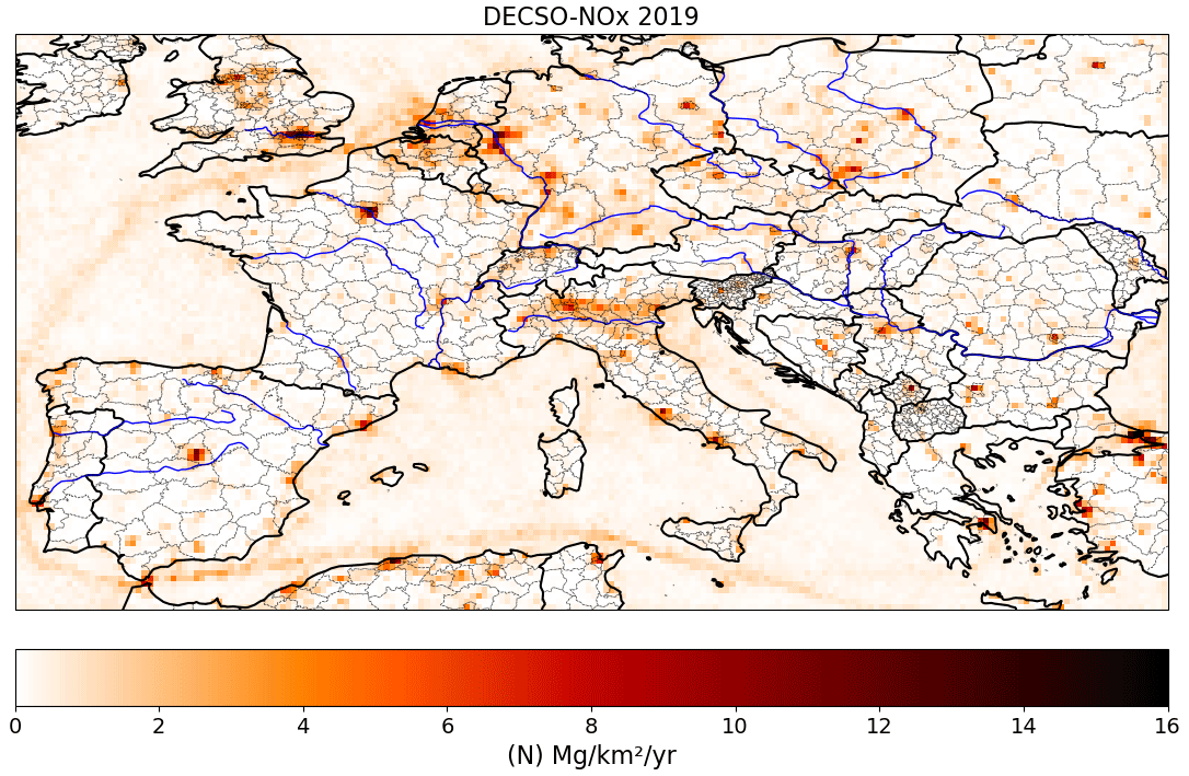
Figure 1 The annually averaged anthropogenic NO_x emissions for 2019 derived from TROPOMI NO₂ observations using the DECSO algorithm.

2.2 Databases for validation

For comparison of the emission results in Europe we will use several inventories, all based on official emissions reported to the European Environment Agency (EEA). The first one is the inventory of national emissions per source category reported under the National Emission reduction Commitments (NEC) Directive of the European Union. Another similar inventory is the emission inventory reported under the Convention on Long-range Transboundary Air Pollution (LRTAP), which gives the country totals of emissions in various source categories. The last one we will use is the European Pollutant Release and Transfer Register (E-PRTR; EPRTR, 2012), which is a database of the individual emissions of the biggest industrial facilities (above 0.1 Mg yr−1) in Europe. The E-PRTR emissions data are reported on an annual basis. From here on we will call these databases simply NEC, LRTAP, and E-PRTR. Besides comparison with these officially reported emissions, we will also compare our emissions to the regional anthropogenic emission inventory CAMS-REG-ANT v5.1 for air quality in Europe (Kuenen et al., 2022) developed for the Copernicus Atmospheric Monitoring Service (CAMS), hereafter called CAMS-REG. For these annual CAMS-REG emissions we use the total emissions regridded from 0.1°×0.05° to 0.2°×0.2° and exclude the soil emissions (i.e. agricultural categories), since soil emissions are also excluded in DECSO. Temporal profiles are also derived in CAMS, which allow us to compare time series for monthly averaged values. We will use the Copernicus Atmosphere Monitoring Service TEMPOral profiles (CAMS-GLOB-TEMPO; Guevara et al., 2021, 2024) for comparison of monthly variations in anthropogenic NO_x emissions. The global emission data version 5.3, called CAMS-GLOB-TEMPO, at a resolution of 0.1°×0.1° has been regridded to 0.2°×0.2° resolution and is hereafter referred to as CAMS-TEMPO.

3 Evaluation of the satellite-derived emissions

3.1 Country-scale intercomparison

The NO_x emissions derived with DECSO have been summed over the countries in our domain and compared to the registered total emissions in NEC and LRTAP. Note that for the national total emissions the spatial resolution or spatial smoothing of the derived emissions plays hardly any role. In total, 21 countries are completely covered by our geographical domain and have reported their emissions. The total anthropogenic emissions (excluding soil emissions) for all these 21 countries are 1.44 (N)Tg yr⁻¹ according to both LRTAP and NEC. The total calculated anthropogenic emissions by DECSO are 1.54 (N)Tg yr⁻¹, about 7 % higher than the reported emissions. The total anthropogenic emissions of CAMS-REG (excluding soil emissions) for the same region are 1.54 (N)Tg yr⁻¹, in agreement with DECSO. Note that the total soil emissions derived by DECSO are 0.78 (N)Tg yr⁻¹ for the same region, but this number cannot be compared because soil emissions in LRTAP and NEC are only given for the agricultural sector and not for forestry. The anthropogenic country totals are shown in Fig. 2. In general, we see a good agreement with the official reported country total emissions of LRTAP and NEC except for Italy, which has much lower reported emissions. Greece, on the other hand, has higher registered emissions, but the mismatch might be related to the difficulty in counting over the Greek islands, since we have weighted the emissions by the land fraction in each grid cell to exclude maritime emissions in these country totals. For CAMS-REG we see bigger deviations not only for Italy but also for Germany, Poland, and Spain. Note that Ireland is only partly in our geographical domain and therefore has lower emissions according to DECSO. Besides the comparison on a national level, good agreement is also found on a provincial scale, as has been shown for Catalonia in the European Commission (EC) project, Sentinel EO-based Emission and Deposition Service (SEEDS).

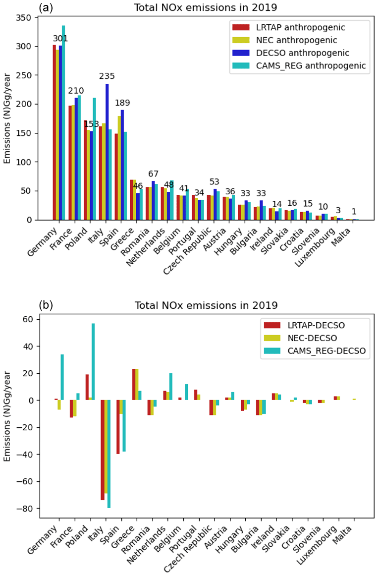
Figure 2 (a) Country totals of anthropogenic NO_x emissions (in (N)Gg yr⁻¹) in the year 2019 according to databases LRTAP, NEC, and CAMS-REG and the DECSO calculations. (b) Differences in total emissions calculated by LRTAP, NEC, and CAMS-REG compared to DECSO.

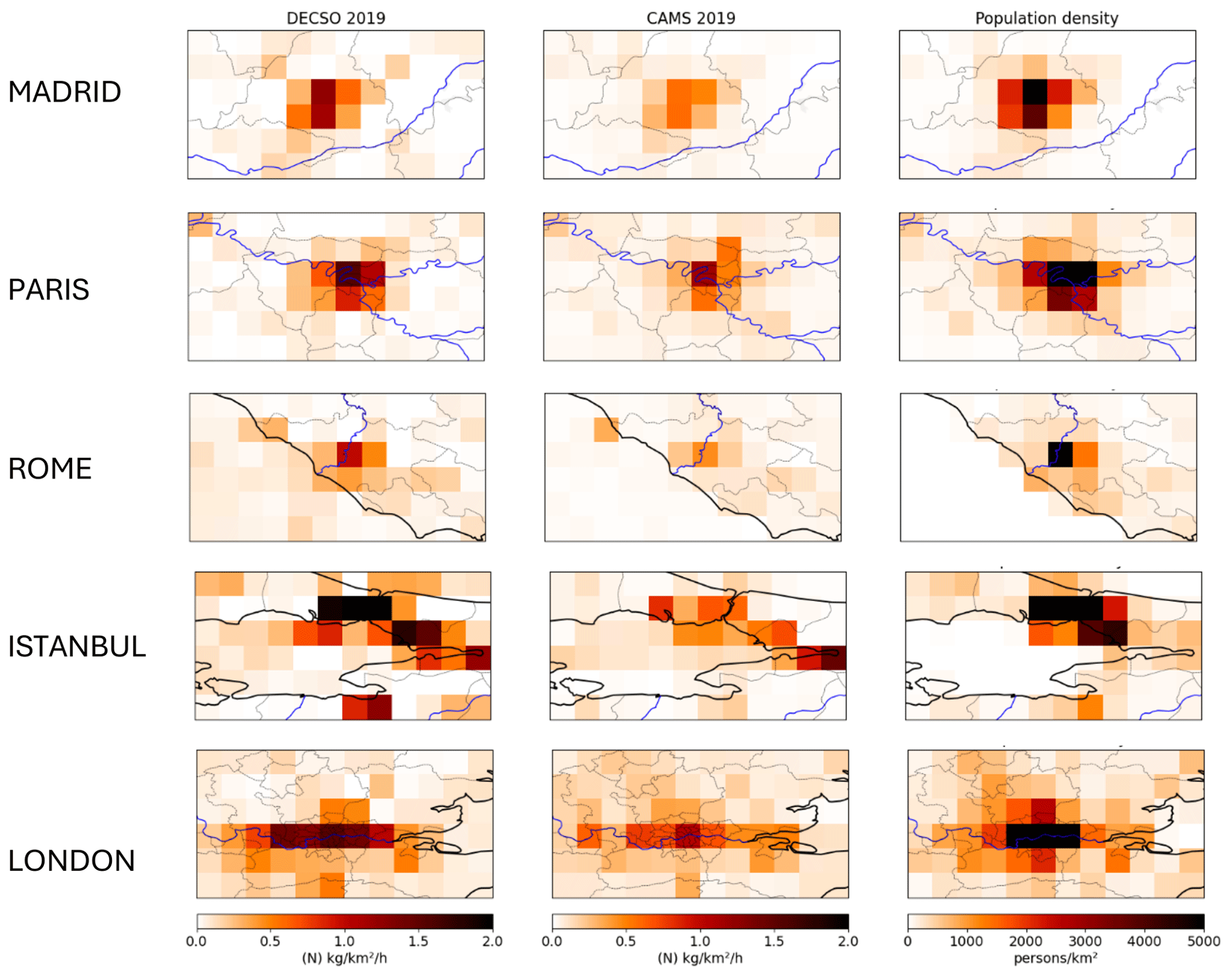
Figure 3 Zoomed-in plots for five large cities in Europe to illustrate the differences in distribution of emissions of DECSO (first column) and CAMS-REG (second column) and the population density (third column) per km².

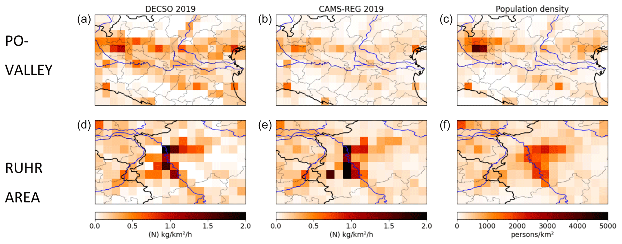
Figure 4 Zoomed-in plots for two large, densely populated, and industrial regions in Europe to illustrate the differences in distribution of emissions of DECSO (a, d) and CAMS-REG (b, e) and the population density (c, f) per km².

3.2 City scale

With our current spatial resolution of 0.2×0.2°, we observe emissions per city district for large cities, but the geographical distribution can be slightly blurred by the 0.2° resolution of the TROPOMI super-observations. Figure 3 shows the spatial distribution of the annual emissions of DECSO and CAMS-REG for five of the largest cities in Europe: Madrid, Paris, Rome, Istanbul, and London. Although DECSO shows similar emissions for the country totals, we see that for large cities DECSO estimates higher emissions in the city centre, and more activities are seen in the region surrounding the city, as compared to the CAMS-REG emissions. The industrial complexes at Rouen located northwest of Paris and at the port of Civitavecchia located west of Rome are similar in DECSO compared to in CAMS-REG. The area of Rouen used to have an active oil refinery, but in recent years the industrial emissions are about 0.11 (N)kg km⁻² h⁻¹ according to the E-PRTR database, which compares well to CAMS-REG and DECSO. The spatial extent of high emissions in the Rome area is smaller in CAMS-REG, which follows the population density more. However, the densely populated centre of Rome is surrounded by a busy ring road with a 20 km radius and a lot of commercial activities around the city, which are not reflected in the population density map. The two power plants at Civitavecchia have reported emissions according to the E-PRTR database which are equivalent to about 0.17 (N)kg km⁻² h⁻¹ per grid cell, which is closer to the DECSO-derived emissions. Although this study focuses mainly on the land emissions, we see in the map for Rome that the maritime emissions of CAMS-REG and DECSO disagree a lot, and this is a topic for further studies. The city emissions in Istanbul are much higher in DECSO than in CAMS-REG. These emissions will include a lot of ship emissions, since it includes the busy ship route through the Bosporus Strait. The map of the greater area of London shows that DECSO has higher emissions in the city but lower emissions outside the city. This is a pattern we see: in general, in most big cities the emissions derived by DECSO show a similar distribution to in CAMS-REG, but the absolute emissions are higher, while the emissions in rural regions are usually lower in DECSO than in CAMS-REG. The lower emissions in the rural regions can be seen in Fig. S1 in the Supplement, which show maps for Europe of both emission products.

In Fig. 4 we show the emissions for two large industrial areas in Europe: the Po Valley and the Ruhr area. For the Po Valley the patterns are similar, but again the DECSO emissions are higher in every city except for Genoa in the southeastern corner of the map. For the Ruhr area, the difference in emissions over cities is small, with the biggest differences located at the big power plants of Weisweiler, Neurath, and Niederaußem around the open-pit lignite mine of Hambach (the largest in Europe). The DECSO emissions are lower than CAMS-REG at the locations of these power plants.

Table 1 Annual NO_x emissions (N)Gg yr⁻¹ of the four lignite power plants. CAMS in the table refers to CAMS-TEMPO.

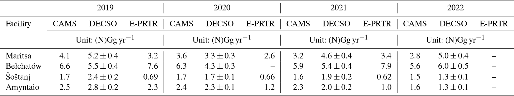
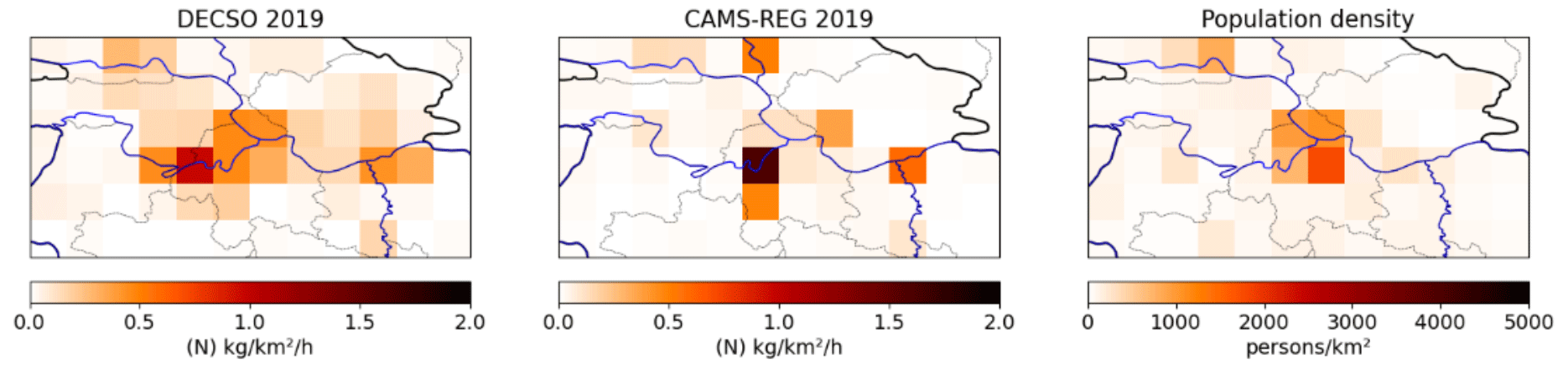
Figure 5 A map of northern Serbia with NO_x emissions of DECSO and CAMS-REG. The population map especially shows the higher population for Belgrade. The emissions in DECSO are mainly correlated with the locations of several coal power plants (Nikola Tesla A, Nikola Tesla B, and Kolubara) and a cement factory (Lafarge in Beočin) in the northwest.

On a European scale the biggest difference between CAMS-REG and DECSO was found for the region around Belgrade in Serbia (Fig. 5). The city of Belgrade is identified by the higher population density in Fig. 5. West of the city, the Nikola Tesla power plants are located, which are strong emitters according to the E-PRTR database. They show up as a strong emission source in the DECSO emissions, but they are mislocated in the current CAMS-REG emissions.

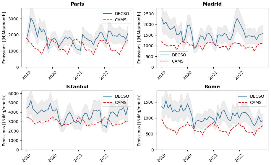
Figure 6 Time series of monthly NO_x emissions derived by DECSO for the cities Paris, Madrid, Istanbul, and Rome in the period 2019 to 2022. The shaded grey area shows the estimated uncertainty in the DECSO emissions. The dashed red line shows the CAMS-TEMPO NO_x emissions for the same grid boxes.

Figure 6 shows examples of time series for city emissions, in this case for the cities of Paris, Madrid, Istanbul, and Rome (also shown in Fig. 3). In these plots we report the total emissions in a square area of 5×5 grid cells centred on the city centre to make sure the whole city has been captured. As seen earlier, the DECSO emissions are on average higher than for CAMS-TEMPO, but the seasonal cycle is also different. The NO_x emissions of CAMS-TEMPO show a seasonal cycle, which is almost identical each year, while DECSO shows larger variations from year to year. We see clearly the effect of COVID regulations in all cities, which started first in March/April 2020 in Europe, and in the winter of 2020–2021 when strict COVID regulations were again in place. The general overall trend in this 4-year time period varies from city to city, but most cities show a slightly decreasing trend, partly related to a gradual decrease in emissions from road vehicles linked to European regulations.

3.3 Intercomparison for large point sources

To evaluate the performance of monitoring emissions from large point sources (LPSs), we compare the DECSO emissions with emissions registered in the E-PRTR database. The isolated LPSs we selected in Europe are all large power plants close to lignite mines. Emissions from DECSO are slightly spread to adjacent grid cells because the spatial resolution of the emission field is less than the sampling of the grid cells, as discussed in Sect. 2. To correct for this, we can deconvolute the emissions around the isolated point source, but here we choose to sum the anthropogenic emissions in the 3×3 grid cells including and around the point source to make sure all emissions are accounted for. For the four cases discussed below, no other significant sources exist in these 3×3 grid cell boxes, and soil emissions are excluded. We estimate the rural anthropogenic emissions in such an area of 3×3 grid cells in Europe to be about 0.13 (N)Gg yr⁻¹ by averaging the emissions of several similar rural 3×3 regions in Europe. We did not correct for this background signal, but we included this in the error bars of Fig. 7.

The first case is that of the Maritsa Iztok facility in Bulgaria located next to an open coal mine. There is no big city or any other industrial facility in the neighbourhood except for the three big power plants of the Maritsa Iztok facility. Figure 7 shows the monthly averaged emissions calculated by the DECSO algorithm and the CAMS-TEMPO inventory and shows the annual emissions from the E-PRTR database for the Maritsa facility. For a fair comparison we also selected for CAMS-TEMPO the same 3×3 grid cells around the LPS. For the period 2019–2022 the annual emissions are given in Table 1 according to DECSO, CAMS-TEMPO, and E-PRTR. The differences in annual emissions between DECSO, CAMS-TEMPO, and E-PRTR of the Maritsa facility are within 20 %–40 %, although DECSO is the highest. The CAMS-TEMPO emissions show a negative trend not visible in DECSO, which shows the highest emissions for 2022. Unfortunately, no E-PRTR data for 2022 are publicly available yet.

The second power plant is the Bełchatów power plant in Poland with its capacity of 5053 MW, the biggest power plant in Europe. It is also one of the most-polluting power plants in the world and gets its fuel from the adjacent lignite coal mine of Bełchatów (Guevara et al., 2024). For the year 2020 no emission values are reported in the current E-PRTR database. For the years 2019 and 2021 DECSO observes high emissions of about 5.5 (N)Gg yr⁻¹, but this is lower than the reported value of more than 7 (N)Gg yr⁻¹. CAMS-TEMPO also shows lower emissions with a negative trend. Godłowska et al. (2023) showed the stack measurements of this power plant in their Fig. 7, which also are in general lower than the E-PRTR values.

The next selected isolated power plant is the Šoštanj lignite power plant in the Velenje basin in a mountainous area of Slovenia. It is responsible for one-third of the electricity need of Slovenia (Božnar et al., 2012). For this LPS both CAMS-TEMPO and DECSO show emissions more than 2 times higher than E-PRTR, which is too large to be explained by the small cities or other small sources located in the neighbourhood.

The last case is that of the power plants of the Ptolemais-Amynteon and Florina coal basins in Western Macedonia, Greece, which were also studied by Skoulidou et al. (2021). There are five power plants associated with and located in this basin, but only three are still active: Agios Dimitrios (1595 MW), Kardia (1200 MW), and Amyntaio (600 MW) (Kostakis, 2009). For 2021 no data were reported for Amyntaio in the E-PRTR database. The reported values of the E-PRTR database match those of CAMS-TEMPO and DECSO quite well, except for the year 2020 that marks the start of a decrease in emissions in this region. The decreasing trend can be seen in all three emission timelines but is strongest in the E-PRTR time series. Most notable in the figure is the strong seasonal cycle in DECSO NO_x emissions for the Greek power plants with the lowest emissions in summertime. This can be related to the availability of more sustainable energy sources in the summer months.

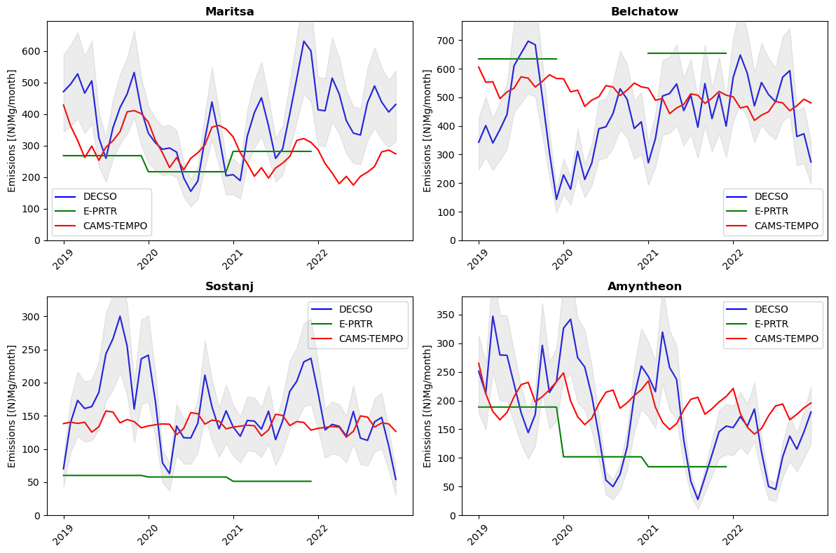
Figure 7 Time series of the NO_x emissions of the selected LPSs in Europe as estimated by DECSO (blue line), E-PRTR (green line), and CAMS-TEMPO (red line). The shaded grey area shows the estimated uncertainty in the DECSO emissions.

From this comparison of several large LPSs in Europe, we see that CAMS-TEMPO and DECSO are often larger than the reported emissions in E-PRTR. In view of the completely different methodologies and the estimated precision of 25 % for DECSO monthly emissions, the annual values of CAMS-TEMPO and DECSO are often in reasonable agreement (within 20 %), but the variability in DECSO is much higher than that of CAMS-TEMPO. Emissions of thermal power plants are more intermittent because of the variability in energy demand and variability in energy supply introduced by solar and wind energy sources (Kubik et al., 2012). Note also that CAMS-TEMPO has the exact same seasonal variability for each of the 4 years, which seems unrealistic. The CAMS-TEMPO emissions in the period 2019 to 2022 show for most studied LPSs a constant negative trend, which was generally not detected in DECSO. Without additional information it is difficult to draw any conclusions on the performance for LPS, but DECSO supplies additional information on these industrial facilities in Europe, and the largest discrepancies may be caused by strong diurnal variability (which TROPOMI observes at about 13:30 LT) and will be interesting for further investigation.

In all cases we see lower emissions in 2020 during the COVID-19 pandemic. In this period the demand for energy was lower, and, while renewable energy output remained similar, the energy from lignite-based power plants was in less demand (Quitzow et al., 2021).

4 Discussion

We presented the latest version of the DECSO algorithm, version 6.3. Updates have been made for the super-observations, the chemical transport model, the sensitivity matrix, and the error parametrization. The new version also includes an error estimate for the monthly NO_x emission data taking into account the autocorrelation in time. The new DECSO version has been applied to the domain of Europe and shows more spatial details than before as a result of the higher resolution of TROPOMI observations compared to earlier satellite observations.

In the comparison with CAMS-REG over Europe (where emissions are usually well-known) the deviations are small (within 10 %) when looking at a country scale. For point sources the spread in the differences is much higher, but no systematic effect has been found yet. For cities DECSO shows higher emissions, while CAMS-REG is higher for rural regions. On a European scale the biggest difference between CAMS-REG and DECSO was found for the region west of Belgrade in Serbia, where the Nikola Tesla power plants are located. While these show up as a strong emission source close to Belgrade in both the DECSO emissions and the E-PRTR database, they are not included or are mislocated in the CAMS-REG emissions. This is a prominent example that demonstrates the value of monitoring emissions with satellite observations.

The precision of the derived emissions by DECSO is given for each grid cell in the data files. In general, we can say that the precision of NO_x emissions given per grid cell (0.2°×0.2°) is about 8 % for annual emissions, 25 % for monthly emissions, and between 10 % and 60 % for the daily emissions. When averaging over a larger domain the precision will, of course, become higher by the square root of the number of grid cells.

The comparison between CAMS-REG and DECSO emissions showed that DECSO is very similar to CAMS-REG for the spatial distribution and the country totals, while compared to the reported emissions in NEC or LRTAP, DECSO is 7 % higher. Validation of the TROPOMI NO₂ observations showed that, when using averaging kernels, the bias of the tropospheric column is estimated as −8 % on average by comparison with MAX-DOAS observations (Keppens and Lambert, 2023). This bias of −8 % should result in lower emissions by DECSO, and the deviation between DECSO and other inventories would be higher in reality. Keppens and Lambert (2023) further report that for polluted regions the mean bias of the TROPOMI NO₂ observations is stronger, about −29 %, while for clean areas the median bias is positive and about +13 % (when using averaging kernels). This would be contradictory to our findings over cities, where DECSO shows higher emissions than CAMS-REG. These lower emissions of CAMS-REG in cities as compared to the rural regions may point to an underestimation of bottom-up traffic emissions, but uncertainties in both satellite observations and bottom-up emissions are in general high. Another potential cause of biases in our emissions is the CHIMERE model. More research is needed for a better understanding of the validation results of TROPOMI observations and CHIMERE performance and of the comparisons between DECSO and CAMS.

This study shows the potential of DECSO for operational emission monitoring for Europe. The monitoring of LPSs is only possible for isolated sources; thus a future improvement can be made by providing the emissions at a higher resolution at the cost of longer processing time. This will allow the study of more isolated LPSs. DECSO has already demonstrated its performance on a 0.1°×0.1° grid for smaller regions like the Yangtze River Delta (Zhang et al., 2023), western Siberia (van der A et al., 2020), and the Netherlands.

In this study the focus was on Europe, but in other regions of the world emissions might be less well known. For these regions DECSO can be or has been applied, since we have global satellite observations. Recently we have applied DECSO to areas in Africa, where several mines with high NO_x emissions were found that were unreported in bottom-up emission inventories like EDGAR or CAMS. This also shows the possibilities for application of DECSO in the Global South.