Uncertainty in simulated brightness temperature due to sensitivity to atmospheric gas spectroscopic parameters from the centimeter- to submillimeter-wave range

Atmospheric radiative transfer models are extensively used in Earth observation to simulate radiative processes occurring in the atmosphere and to provide both upwelling and downwelling synthetic brightness temperatures for ground-based, airborne, and satellite radiometric sensors. For a meaningful comparison between simulated and observed radiances, it is crucial to characterize the uncertainty in such models. The purpose of this work is to quantify the uncertainty in radiative transfer models due to uncertainty in the associated spectroscopic parameters and to compute simulated brightness temperature uncertainties for millimeter- and submillimeter-wave channels of downward-looking satellite radiometric sensors (MicroWave Imager, MWI; Ice Cloud Imager, ICI; MicroWave Sounder, MWS; and Advanced Technology Microwave Sounder, ATMS) as well as upward-looking airborne radiometers (International Submillimetre Airborne Radiometer, ISMAR, and Microwave Airborne Radiometer Scanning System, MARSS). The approach adopted here is firstly to study the sensitivity of brightness temperature calculations to each spectroscopic parameter separately, then to identify the dominant parameters and investigate their uncertainty covariance, and finally to compute the total brightness temperature uncertainty due to the full uncertainty covariance matrix for the identified set of relevant spectroscopic parameters. The approach is applied to a recent version of the Millimeter-wave Propagation Model, taking into account water vapor, oxygen, and ozone spectroscopic parameters, though the approach is general and can be applied to any radiative transfer code. A set of 135 spectroscopic parameters were identified as dominant for the uncertainty in simulated brightness temperatures (26 for water vapor, 109 for oxygen, none for ozone). The uncertainty in simulated brightness temperatures is computed for six climatology conditions (ranging from sub-Arctic winter to tropical) and all instrument channels. Uncertainty is found to be up to few kelvins [K] in the millimeter-wave range, whereas it is considerably lower in the submillimeter-wave range (less than 1 K).

1 Introduction

Radiative transfer models (RTMs) are widely used to compute the propagation of electromagnetic radiation through the Earth’s atmosphere and to simulate radiometric observations of natural radiation (Rosenkranz, 1993). At the core of RTMs are atmospheric absorption models, which simulate the absorption and emission of electromagnetic radiation by atmospheric constituents. RTMs represent the forward operator for atmospheric radiometric applications. Thus, RTMs are widely exploited for the solution of the inverse problem, i.e., the retrieval of atmospheric parameters from radiometric observations (Rodgers, 2000), and for data assimilation of radiometric observations in numerical weather prediction (NWP) models (Saunders et al., 2018). In addition, as part of their quality control, radiometric observations from satellites are often validated against simulated radiances obtained by processing thermodynamic profiles from radiosondes or NWP models with RTMs (Clain et al., 2015; Kobayashi et al., 2017). Therefore, RTMs and absorption models have general application for atmospheric sciences, including meteorology and climate studies. All these applications would benefit from a careful characterization of RTM uncertainty. For example, instrument validation through comparison of observations and simulations should take the uncertainty in both to be metrologically meaningful (Bodeker et al., 2016; Yang et al., 2023). However, the characterization of uncertainty associated with simulated brightness temperatures is generally lacking within the scientific literature. This work aims to fill this gap, providing a thorough analysis of the uncertainty in simulated brightness temperatures due to assumptions in the atmospheric absorption model.

Synthetic brightness temperatures (T_B) simulated with atmospheric radiative transfer and absorption models are inherently affected by uncertainty due to the assumed values for the intrinsic spectroscopic parameters. These values are in fact determined from theoretical calculations, lab experiments, or field measurements and are thus affected by either computational or experimental uncertainty. This uncertainty then propagates from the spectroscopic parameters through the absorption model and RTM calculations and finally to simulated T_B and atmospheric retrievals. It is therefore crucial to provide an estimate of the T_B uncertainty value in order to have an adequate interpretation of the observation-minus-simulation statistics and to fulfill international standard requirements.

Therefore, the rationale for this work is to fully characterize the synthetic T_B uncertainty due to the uncertainty in atmospheric gas spectroscopic parameters, following the approach proposed by Cimini et al. (2018). In particular, the scope is to assess the uncertainty in the synthetic brightness temperatures obtained via the Millimeter-wave Propagation Model based on the spectroscopy from Rosenkranz (2019). The approach consists of mapping the uncertainty in the T_B to each single spectroscopic parameter. The analysis is performed in four steps: (i) review the open literature concerning spectroscopic parameters relevant for the frequency range of interest (16–700 GHz) for assessing the associated uncertainties (this can be found in Turner et al., 2022), (ii) perform a sensitivity study to investigate the dominant uncertainty contribution to radiative transfer calculations, (iii) estimate the full uncertainty covariance matrix for the reduced set of dominant parameters, and (iv) propagate the uncertainty covariance matrix to estimate the impact on simulated brightness temperatures. We perform the above analysis for the estimation of the uncertainty in simulated brightness temperature in the frequency range 16–700 GHz, both for the downward-looking view at 53° from nadir at the top of atmosphere (TOA) – i.e., the observation geometry of the EUMETSAT Polar System Second Generation (EPS-SG) MicroWave Imager (MWI) and Ice Cloud Imager (ICI) – and for the zenith upward-looking view from different heights, as feasible for airborne sensors. The estimated uncertainty spectra are also convolved on the finite channel bandwidths of the relevant satellite and airborne instruments. For the downward-looking geometry, we consider MWI and ICI, as well as the EPS-SG MicroWave Sounder (MWS) and the Advanced Technology Microwave Sounder (ATMS) aboard NOAA satellites (Suomi NPP, NOAA-20, NOAA-21). For the upward-looking geometry, we consider selected channels from the International Submillimetre Airborne Radiometer (ISMAR) (Fox et al., 2017) and the Microwave Airborne Radiometer Scanning System (MARSS) (McGrath and Hewison, 2001).

The motivation for selecting the above frequency range and instruments is explained below. The EPS-SG will contribute with a new generation of polar-orbiting satellites in the timeframe from 2025 onward (Accadia et al., 2020; Mattioli et al., 2019), providing continuity to the current EUMETSAT EPS program. For the EPS-SG a number of missions have been identified, which include the aforementioned MWI, ICI, and MWS missions. This study is indeed in preparation for and support of the calibration and validation activities and exploitation of these missions, and it focuses on the quantitative assessment of atmospheric absorption model uncertainty in the frequency range encompassing the instruments' channels of interest (i.e., 16–700 GHz). The outcome of this study will also be applicable to ATMS, as representative of commonly used microwave instruments currently in operation. The airborne instruments are used as demonstrators for the EPS-SG.

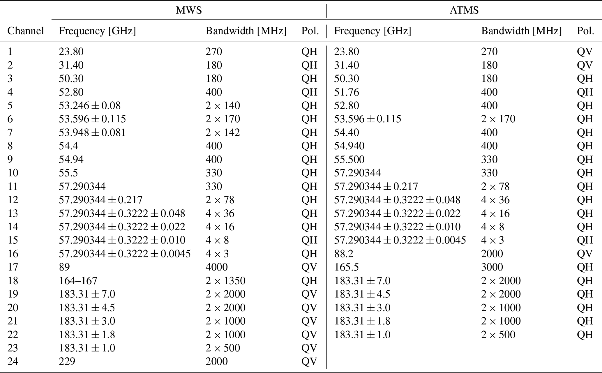
MWI and ICI are two conically scanning microwave radiometers. MWI will have 18 channels ranging from 18 to 183 GHz, providing continuity of key microwave imager missions. Four channels at 18.7, 23.8, 31.4, and 89 GHz provide key information on weather forecasting, as well as precipitation, total column water vapor, and cloud liquid water. MWI also includes a new set of channels near 50–60 GHz and at 118 GHz, allowing retrieval of weak precipitation and snowfall. ICI is instead specifically designed to support remote sensing of cloud ice and constitutes a novelty of this kind. ICI frequencies will cover the millimeter–submillimeter range spectrum from 183 to 664 GHz: 11 channels in the water vapor absorption lines (i.e., 183, 325, and 448 GHz) compared to 243 and 664 GHz in atmospheric windows. ICI information on humidity and ice hydrometeors will be crucial to characterize cloud properties. The rotation of the slanted antennas allows conical scans with constant incidence angles of about 53°, depending on the channel frequency. MWS is a cross-track scanning radiometer. MWS will comprise 24 channels from 23.8 to 229 GHz. The 14 oxygen-band channels near 50–60 GHz provide microwave temperature sounding, while the water vapor channel at 23.8 GHz and the five channels at 183.31 GHz are used for humidity retrievals. The instrument also carries a new channel at 229 GHz. Both the microwave sounders MWS and ATMS provide information about thermodynamics of the atmosphere, such as temperature and moisture profiles. The microwave sounders MWS and ATMS are both based on a cross-track sensing mechanism, so the Earth is observed at different scanning angles, symmetric around the nadir direction, with an angular sampling spaced by 1.05° and a maximum scanning angle of 49.31°.

To the best of our knowledge, this is the first study investigating the characterization of synthetic upwelling T_B uncertainty due to the sensitivity of gas spectroscopic parameters. Moreover, it extends the work of Cimini et al. (2018, 2019), providing downwelling T_B uncertainty at different heights and to a wide range of frequencies covering the microwave–millimeter-wave range, 16–700 GHz. Although this study adopts the same underlying approach as in Cimini et al. (2018, 2019), it differs in the (i) viewing geometry (satellite/airborne vs. ground-based); (ii) absorption model (featuring new spectroscopy, with additional parameters being investigated); and (iii) frequency range, extended by 1 order of magnitude. Note that a thorough characterization of the uncertainty affecting the simulated brightness temperatures implies better understanding of their limitations when used for the training of inverse algorithms, the monitoring of sensor calibration, and the data assimilation of real observations into NWP models.

The paper is organized as follows: Sect. 2 introduces the theoretical basis and reports on the absorption model sensitivity analysis to spectroscopic parameters; Sect. 3 discusses the implications of spectral channel convolution; Sect. 4 reports on the estimation of the full uncertainty covariance matrix for the spectroscopic parameters; Sect. 5 presents the results of the uncertainty propagation from spectroscopic parameters to simulated T_B; finally, Sect. 6 presents a summary and draws final conclusions.

2 Sensitivity analysis

In this section we briefly introduce the theoretical basis underlying the calculation of the modeled brightness temperature uncertainty, propagating the spectroscopic parameters' uncertainty into the simulated brightness temperature following the method outlined in Cimini et al. (2018). The method first involves a review of the spectroscopic parameters and their uncertainty and then a sensitivity analysis to identify the dominant contributions.

This study exploits a state-of-the-art microwave radiative transfer model, applicable to airborne as well as ground-based and satellite observation geometries. We will adopt the Millimeter-wave Propagation Model using the atmospheric absorption equations by Rosenkranz (1993), with updated spectroscopic parameters, which will be referred to as PWR19 (see also Larosa et al., 2024, for code implementation). The brightness temperature simulated with this model is generally a function of the spectroscopic parameters considered within the model. Under the assumption of small perturbations, non-linear dependence can be reasonably linearized as

$$\begin{array}{}\text{(1)}& {\mathit{T}}_{\mathrm{B}}={\mathbf{K}}_p\cdot \left(\mathit{p}-{\mathit{p}}_{\mathrm{0}}\right)+{\mathit{T}}_{\mathrm{B},\mathrm{0}},\end{array}$$

where p is a vector whose elements are the parameters in the model, with nominal value p₀; T_B is a vector of calculated brightness temperatures at various frequencies using parameter values p, while T_B,0 is calculated for parameter values p₀; and K_p represents the model parameter Jacobian, i.e., the matrix of partial derivatives of model output with respect to model parameters p.

The approach adopted here to compute the T_B uncertainty due to the uncertainties in all gas spectroscopic parameters within the model consists firstly in identifying the dominant parameters causing the uncertainty to reduce the dimensionality of the problem. Hence, we investigate the sensitivity of the model to each spectroscopic parameter, separately, by perturbing the value of that parameter by its estimated uncertainty: if the sensitivity is above a given threshold, the parameter is deemed relevant and considered for further analysis; otherwise it is discarded. We choose to set the threshold equal to 0.1 K, typically below the uncertainty for radiometric observations.

Cimini et al. (2018)Turner et al. (2022)Cimini et al. (2018)Cimini et al. (2018)Turner et al. (2022)Turner et al. (2022)Cimini et al. (2018)Turner et al. (2022)Cimini et al. (2018)Turner et al. (2022)Turner et al. (2022)Turner et al. (2022)Turner et al. (2022)Turner et al. (2022)Turner et al. (2022)Turner et al. (2022)

Table 1 List of water vapor parameters perturbed in the sensitivity analysis.

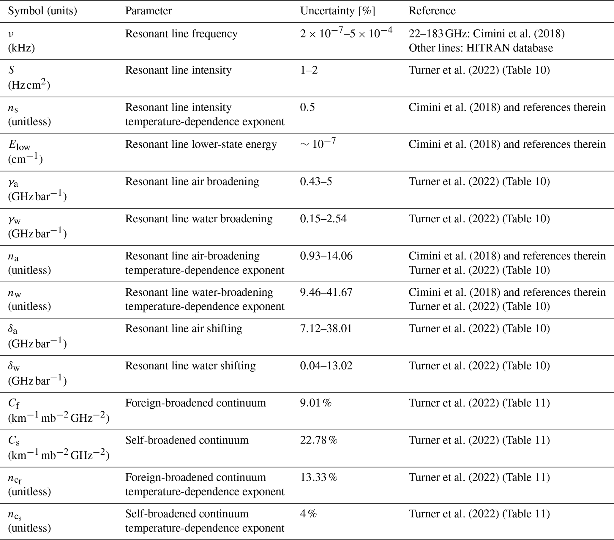
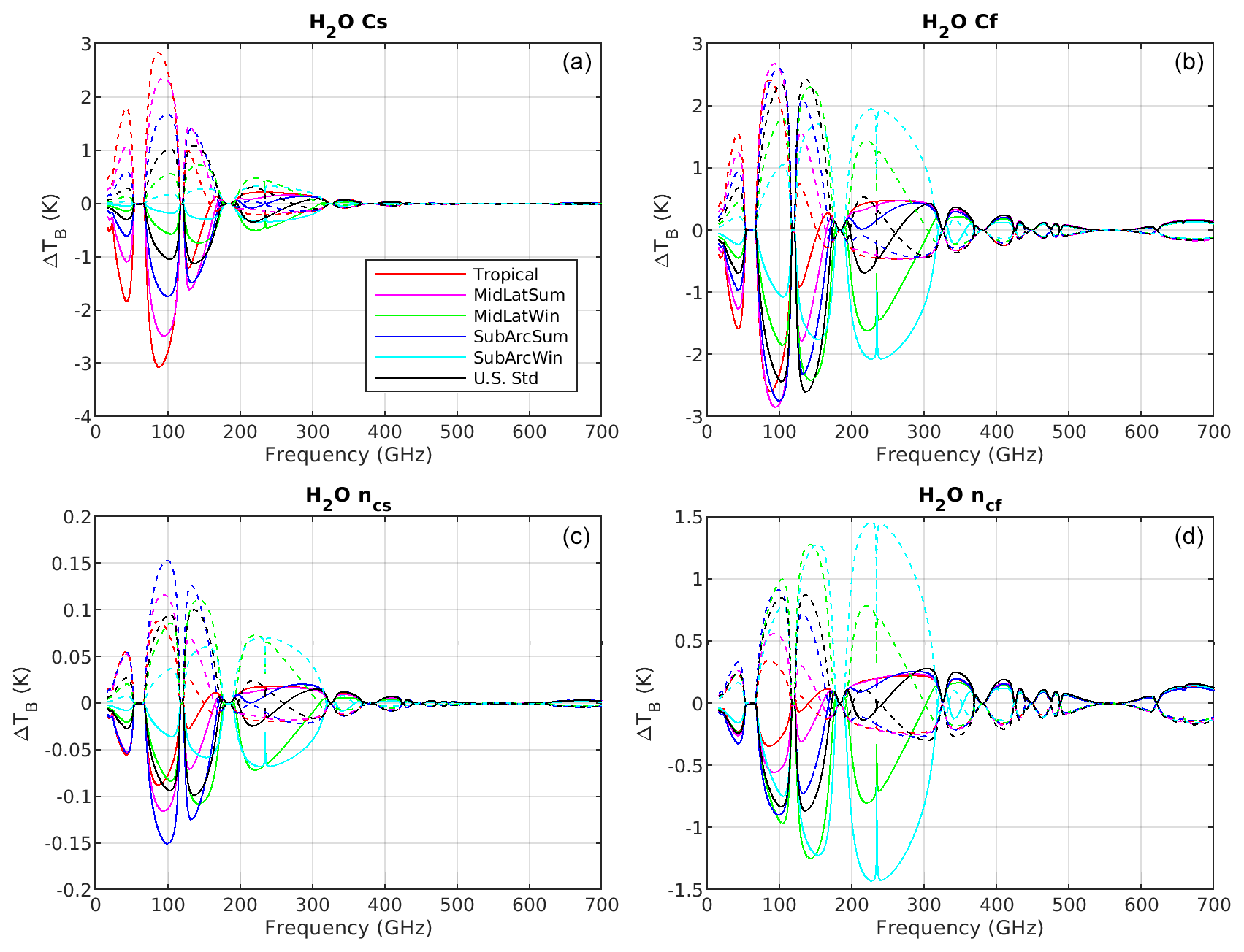
Figure 1 Sensitivity of modeled T_B to water vapor continuum absorption parameters, for downward-looking geometry at 53° from nadir, with H-pol sea surface emissivity. Solid lines correspond to negative perturbation ($\mathrm{\Delta }{\mathit{T}}_{\mathrm{Bi},-}$) and dashed lines to positive perturbation ($\mathrm{\Delta }{\mathit{T}}_{\mathrm{Bi},+}$). Top: self-induced (C_s) (a) and foreign-induced (C_f) (b) broadening coefficients. Bottom: self-broadening (c) and foreign-broadening (d) temperature-dependence exponents ($n_{{\mathrm{c}}_{\mathrm{s}}}$ and $n_{{\mathrm{c}}_{\mathrm{f}}}$, respectively). Different colors indicate six different climatology conditions.

Once we have singled out the reduced set of relevant parameters, the full uncertainty covariance matrix (Cov (p)) is estimated by considering the possible correlations between the spectroscopic parameters. Then, the Jacobian of the radiative transfer model with respect to dominant spectroscopic parameters (K_p) is computed by small-perturbation analysis. Finally, indicating with ^⊺ the matrix transpose, the full uncertainty covariance matrix for the computed brightness temperature is derived from Cov(p) and K_p as (BIPM et al., 2008)

$$\begin{array}{}\text{(2)}& \mathrm{Cov}\left({\mathit{T}}_{\mathrm{B}}\right)={\mathbf{K}}_p\cdot \mathrm{Cov}\left(\mathit{p}\right)\cdot {\mathbf{K}}_p^{⊺}.\end{array}$$

In this work we only consider spectroscopic parameters exploited in PWR19, unless otherwise specified. As anticipated before, the model sensitivity to a given parameter is computed by perturbing the value of that parameter by the estimated uncertainty (at 1σ level). Each parameter has been investigated individually by perturbing its value by ±σ (1σ) uncertainty and computing the impact on the modeled T_B as the difference between T_B computed with the nominal value of the parameter and T_B computed with the perturbed value; i.e.,

$$\begin{array}{}\text{(3)}& \mathrm{\Delta }{\mathit{T}}_{\mathrm{Bi},+/-}={\mathit{T}}_{\mathrm{B}}\left(p_{\mathrm{i}}\right)-{\mathit{T}}_{\mathrm{B}}(p_{\mathrm{i}}\pm {\mathit{\sigma }}_{p_{\mathrm{i}}}).\end{array}$$

Monochromatic radiative transfer calculations are performed in the 16–700 GHz range at 50 MHz resolution, with the addition of selected frequencies corresponding to the central frequency of MWI and ICI (Table 4) and MWS and ATMS channels (Table 5). Six different climatology conditions are considered to account for temperature, pressure, and humidity dependence: tropical, midlatitude summer, midlatitude winter, sub-Arctic summer, sub-Arctic winter, and US standard profiles (Anderson et al., 1986). Thus, for each parameter, both ${\mathit{T}}_{{\mathrm{B}}_{\mathrm{i},+}}$ and ${\mathit{T}}_{{\mathrm{B}}_{\mathrm{i},-}}$ are computed for each of the six typical climatology conditions. For downward-looking geometry, the surface emissivity must be modeled to compute ${\mathit{T}}_{{\mathrm{B}}_{\mathrm{i},+/-}}$. In general we expect the higher the emissivity, the lower the sensitivity to spectroscopic parameters. In fact, a higher emissivity leads to a lower contribution of downwelling radiation to the radiation reaching a satellite downward-looking instrument; thus the sensitivity to spectroscopic parameters is reduced to the upwelling path only. Since oceans cover about 70 % of the Earth, the surface emissivity is modeled over water, using the Tool to Estimate Sea-Surface Emissivity from Microwaves to sub-Millimeter waves (TESSEM²; Prigent et al., 2017). The emissivity is computed at 53° from nadir, corresponding to the ICI and MWI observing angle, assuming typical ocean conditions (8 m s⁻¹ wind speed; 290 K sea surface temperature; 35 PSU salinity). TESSEM² provides emissivity at both H and V polarizations (H-pol and V-pol, respectively), with the emissivity at H-pol lower than at V-pol in the frequency range of interest. Most of the MWI and ICI channels are V-pol (except for window channels featuring both H and V); however, for figure clarity, we consider only the most conservative case, i.e., H-pol emissivity (as previously stated, lower emissivity leads to higher sensitivity). So, hereafter figures show simulations obtained with H-pol emissivity, whereas the reader is referred to the tables in Appendix A for comparison between the two polarizations.

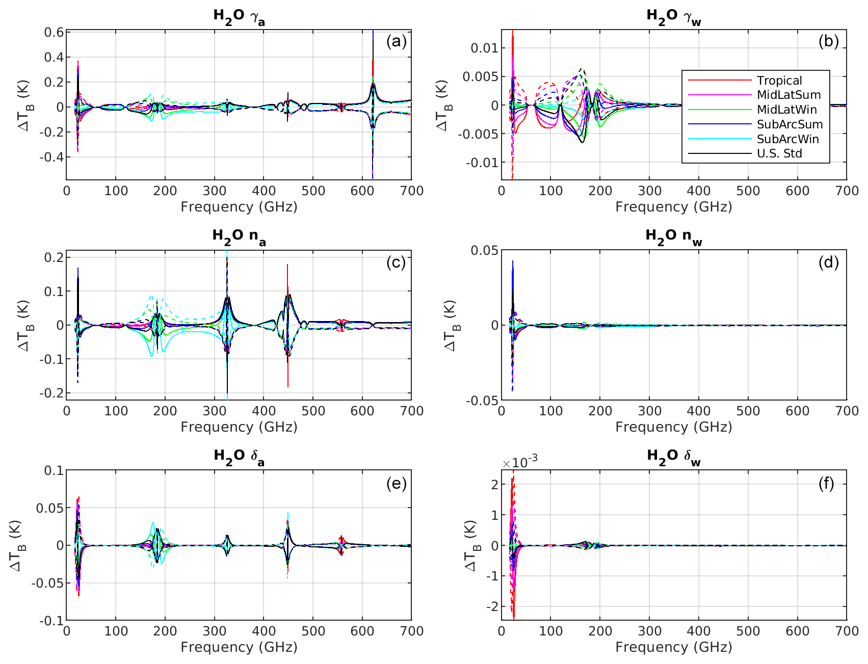
Figure 2 As in Fig. 1 but for water vapor line absorption and broadening and shifting parameters. Solid lines correspond to negative perturbation ($\mathrm{\Delta }{\mathit{T}}_{\mathrm{Bi},-}$) and dashed lines to positive perturbation ($\mathrm{\Delta }{\mathit{T}}_{\mathrm{Bi},+}$). Top: air-induced (γ_a) (a) and water-induced (γ_w) (b) broadening coefficients. Middle: temperature-dependence exponents of air-induced (n_a) (c) and water-induced (n_w) (d) broadening. Bottom: air-induced (δ_a) (e) and water-induced (δ_w) (f) shifting coefficients.

The following sections introduce the spectroscopic parameters of the relevant gases in the considered frequency range, i.e., H₂O, O₂, and O₃, with selected examples of the corresponding ${\mathit{T}}_{{\mathrm{B}}_{\mathrm{i},+}}$ and ${\mathit{T}}_{{\mathrm{B}}_{\mathrm{i},-}}$ spectra. Other uncertainty sources, such as uncertainties in uncertainties or the uncertainties from minor absorbers/lines, are considered second-order contributions; since uncertainty adds up in quadrature, second-order contributions add relatively little with respect to first-order contributions.

2.1 Sensitivity to H₂O parameters

This section investigates the RTM sensitivity to water vapor spectroscopic parameters. In the frequency range under consideration, several resonant lines (from 22 to 916 GHz) contribute non-negligibly to the water vapor absorption. In addition, a non-resonant contribution is given by the so-called water vapor continuum absorption. For the resonant absorption, the following parameters are relevant: line frequency (ν), intensity (S), the temperature dependence of the partition sum (n_S) (i.e., the total number of populated molecular states), the lower-state energy (E_low), air and water broadening (γ_a and γ_w) and their temperature-dependence exponents (n_a and n_w), and air and water shifting (δ_a and δ_w). For the continuum absorption, four parameters are relevant, namely the self- and foreign-induced intensity coefficients and their respective temperature-dependence exponents (C_s, C_f, n_cs, n_cf). Note that this model for the water vapor continuum absorption was specifically developed to address the microwave range and later extended to higher frequencies. However, more recently new models have been proposed based on measurements and ab initio calculations to improve the fits in the millimeter-wave range (Odintsova et al., 2017; Koroleva et al., 2021). However, the dominant foreign continuum fits the f² dependence up to 1 THz well, as reviewed recently (Koroleva et al., 2021). The water vapor parameters perturbed in the sensitivity analysis are listed in Table 1, together with the references from which their values, and estimated uncertainty is derived (i.e., Cimini et al., 2018; Turner et al., 2022, and references therein). It is noted that uncertainty ranges are indicated in Tables 1–3 when the uncertainty value of the spectroscopic parameter depends upon the specific resonant line.

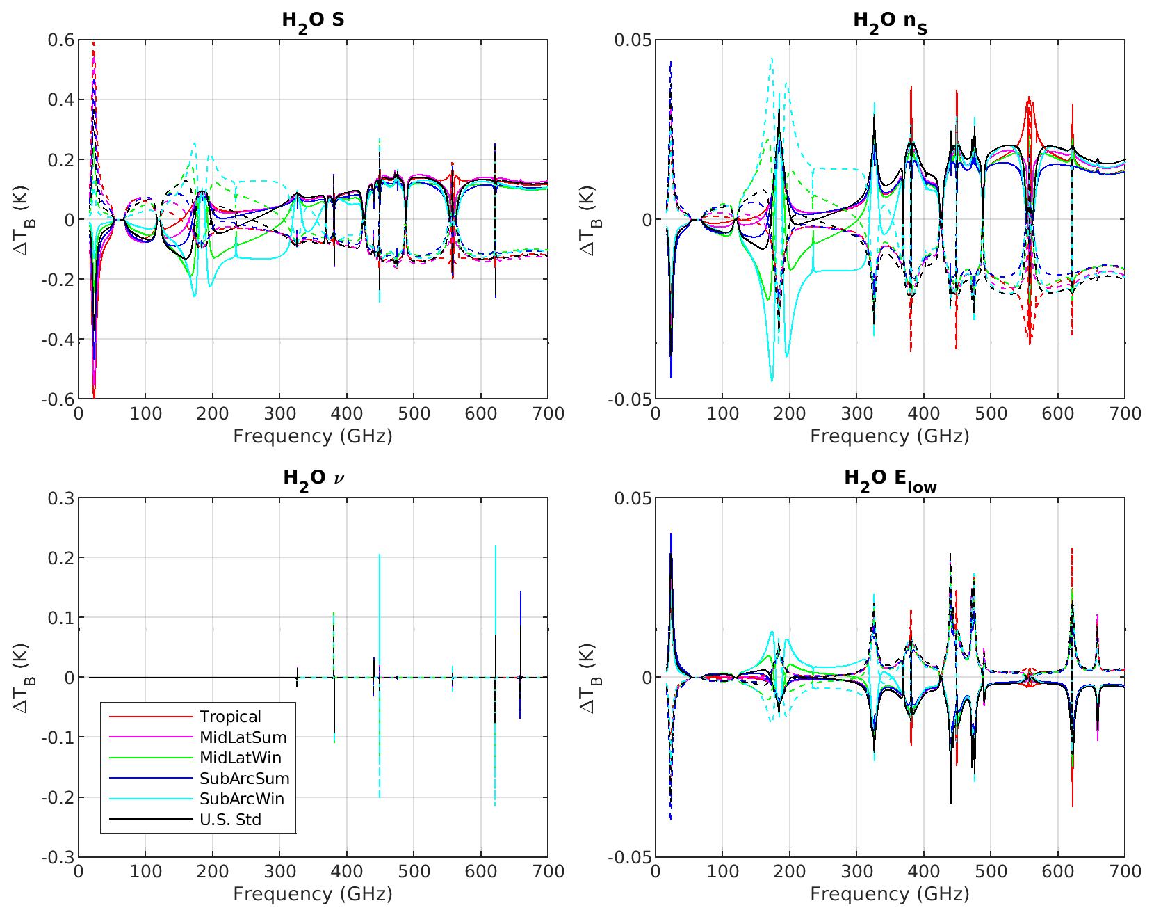
Figure 3 As in Fig. 2 but for line intensity (S), its temperature dependence (n_S), the central frequency (ν), and the lower-state energy (E_low).

Figure 1 shows the $\mathrm{\Delta }{\mathit{T}}_{\mathrm{Bi},+/-}$ spectra corresponding to the perturbation of the four parameters used to model the water vapor continuum absorption (C_s, C_f, $n_{{\mathrm{c}}_{\mathrm{s}}}$, $n_{{\mathrm{c}}_{\mathrm{f}}}$). Each panel shows the sensitivity of modeled 16–700 GHz T_B to one parameter only, as computed for the six climatology conditions. The symmetry of $\mathrm{\Delta }{\mathit{T}}_{\mathrm{Bi},+}$ and $\mathrm{\Delta }{\mathit{T}}_{\mathrm{Bi},-}$ with respect to the zero line suggests that estimated uncertainties represent small perturbations satisfying the linearization assumed above.

Similarly, Fig. 2 shows the $\mathrm{\Delta }{T}_{\mathrm{Bi},+}$ and $\mathrm{\Delta }{T}_{\mathrm{Bi},-}$ spectra corresponding to the perturbation of the broadening and shifting parameters used to model the water vapor line absorption (γ_a, γ_w, n_a, n_w, δ_a, δ_w), while Fig. 3 shows the perturbation of the line intensity (S), its temperature dependence (n_S), the central frequency (ν), and the lower-state energy (E_low). We perturbed the parameters of the six key stronger water vapor lines together. If the impact is less than 0.1 for all, then the parameter is discarded. If the impact is higher than 0.1 for any of them, then the parameter is evaluated for each line, and only those with impact higher than 0.1 K are retained for further analysis. The sensitivity analysis shows that among the model parameters that were perturbed by the estimated uncertainty (Table 1), only eight types impact the modeled upwelling 16–700 GHz T_B by more than 0.1 K: the four continuum parameters (C_s, C_f, $n_{{\mathrm{c}}_{\mathrm{s}}}$, $n_{{\mathrm{c}}_{\mathrm{f}}}$) and four line parameters (γ_a, n_a, S, ν). Among the latter, the central frequency ν will not be considered for the reasons explained in Sect. 3. The other three parameters have been considered for six key water vapor lines (i.e., 22, 183, 325, 448, 556, 752 GHz). In addition, the following line parameters were found to be relevant (ΔT_B>0.1 K):

• S for 380, 474, and 620 GHz;

• γ_a for 620 GHz.

Therefore, 26 parameters were identified as dominant for H₂O absorption uncertainty and are further considered for evaluation of their covariance in Sect. 4.

2.2 Sensitivity to O₂ parameters

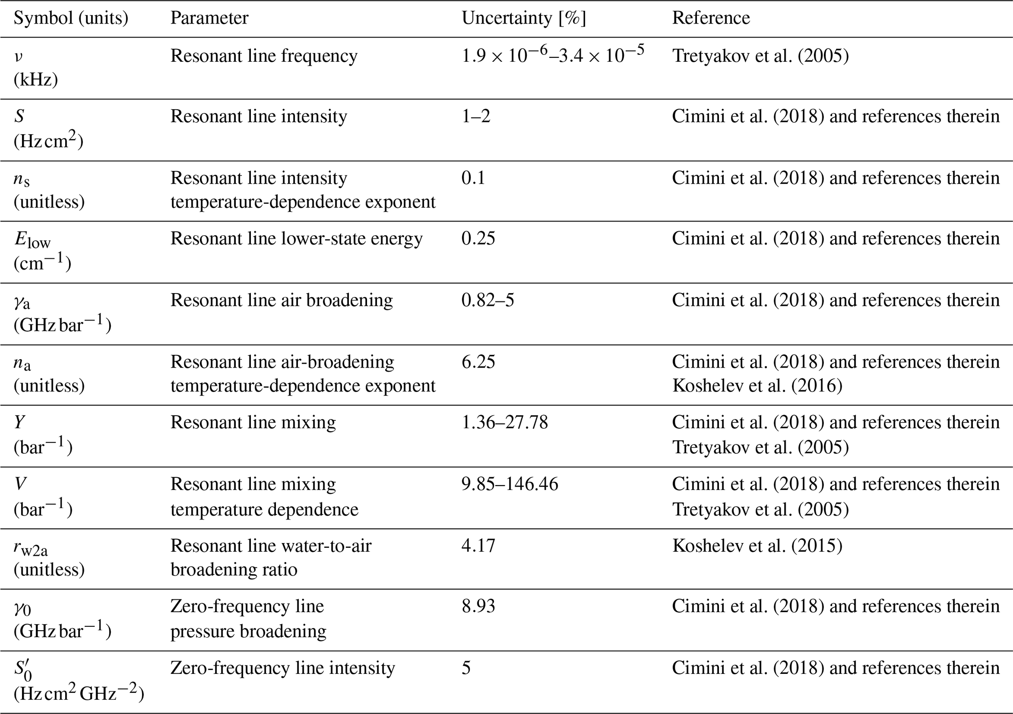
Oxygen contributes to the absorption with several resonant lines in the frequency range under consideration. The PWR19 model includes 49 oxygen absorption lines, of which 37 are within the 60 GHz band; 1 lies at 118 GHz and the remaining 11 are in the millimeter–submillimeter range (200–900 GHz). In addition, the non-resonant contribution is given by a zero-frequency transition; i.e., the O₂ non-resonant contribution is modeled as a pseudo-line at zero frequency (van Vleck, 1947), as discussed in Cimini et al. (2018). For the resonant absorption, the following parameters are relevant: line frequency (ν), intensity (S) and its temperature coefficient (n_S), the lower-state energy (E_low), air broadening (γ_a) and its temperature-dependence exponent (n_a), the normalized mixing coefficient (Y) and its temperature-dependence coefficient (V), and the water-to-air broadening ratio (r_ω2a). For the zero-frequency absorption, two parameters are relevant, the intensity ($S_{\mathrm{0}}^{\prime }$) and broadening (γ₀) of the pseudo-line. This pseudo-line is collisionally coupled with the 60 GHz band (Tretyakov and Zibarova, 2018), although the impact is likely insignificant. Note that $S_{\mathrm{0}}^{\prime }$ corresponds to a different definition of line intensity, which has a finite nonzero value as ν₀→0:

$$\begin{array}{}\text{(4)}& S_{\mathrm{0}}^{\prime }T=\underset{{\mathit{\nu }}_{\mathrm{0}}\to \mathrm{0}}{lim}{\displaystyle \frac{S_{\mathrm{0}}T}{{\mathit{\nu }}_{\mathrm{0}}^{\mathrm{2}}}}.\end{array}$$

The values and uncertainties for the oxygen parameters are either from Tretyakov et al. (2005) (Table 5) or estimated from an independent analysis of measurement methods (Cimini et al., 2018, and references therein). The oxygen parameters perturbed in the sensitivity analysis are listed in Table 2 (first-order expansion of the line mixing parameters is adopted, as in Tretyakov et al., 2005).

Tretyakov et al. (2005)Cimini et al. (2018)Cimini et al. (2018)Cimini et al. (2018)Cimini et al. (2018)Cimini et al. (2018)Koshelev et al. (2016)Cimini et al. (2018)Tretyakov et al. (2005)Cimini et al. (2018)Tretyakov et al. (2005)Koshelev et al. (2015)Cimini et al. (2018)Cimini et al. (2018)

Table 2 List of oxygen parameters perturbed in the sensitivity analysis.

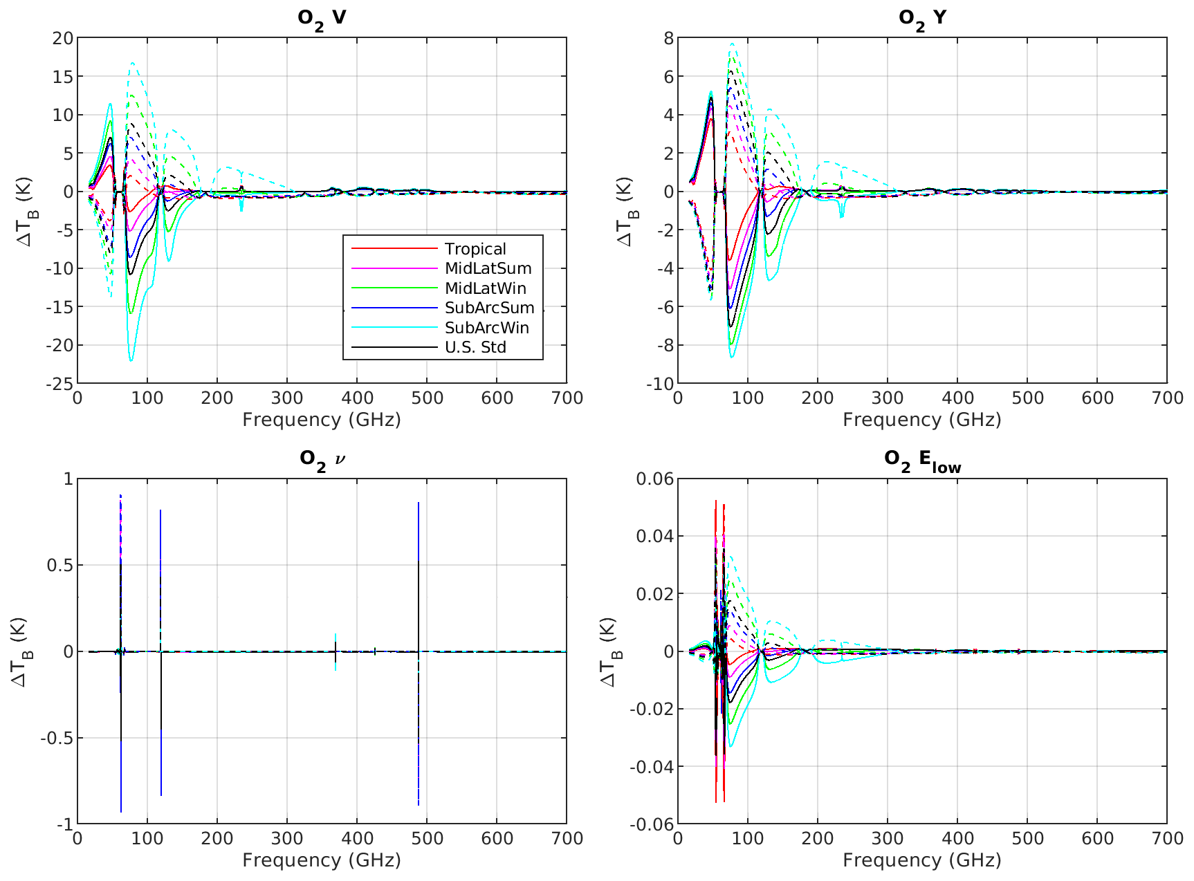
Figures 4–5 show the $\mathrm{\Delta }{\mathit{T}}_{\mathrm{Bi},+}$ and $\mathrm{\Delta }{\mathit{T}}_{\mathrm{Bi},-}$ spectra corresponding to the perturbation to four oxygen line absorption parameter, (S, $S_{\mathrm{0}}^{\prime }$, γ₀, γ_a) and V, Y, ν, and E_low, respectively. The sensitivity analysis shows that among the model parameters in Table 2, which were perturbed by the estimated uncertainty, only the following impact the modeled upwelling 16–700 GHz T_B more than 0.1 K: two for the zero-frequency non-resonant absorption (S′₀, γ₀), four for the line position and absorption (ν, S, γ_a, n_a), and two for the line mixing (Y, V). Among these, the central frequency ν will not be considered for the reasons explained in Sect. 3. Parameters of weak oxygen lines in the 60 GHz band are included along with the strong lines because their covariance can be analyzed by the same algorithm, without incurring additional labor (except by the computer). Therefore, 109 parameters were identified as dominant for O₂ absorption uncertainty and are further considered for evaluation of their covariance in Sect. 4.

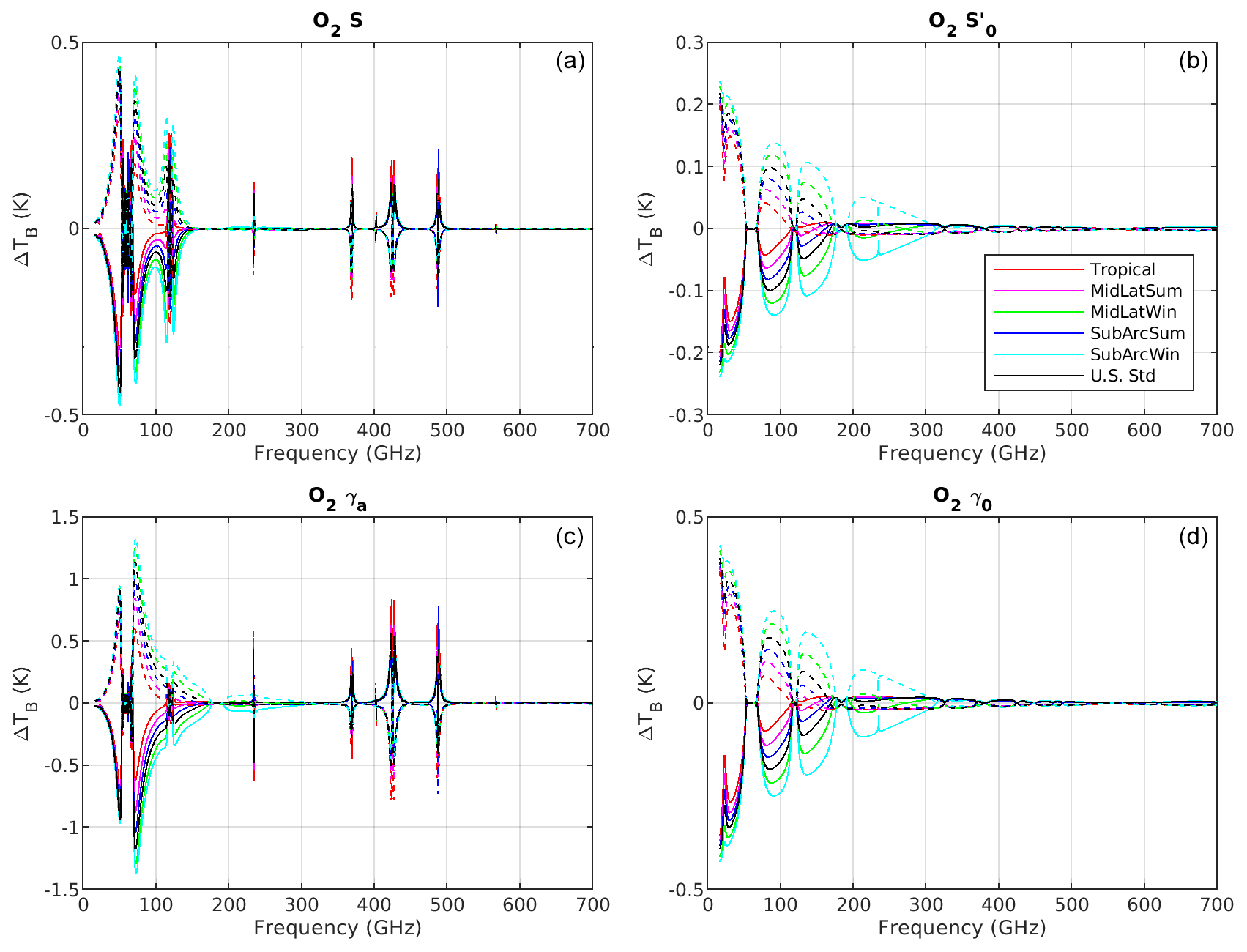
Figure 4 Sensitivity of modeled T_B to oxygen line absorption parameters. Solid lines correspond to negative perturbation ($\mathrm{\Delta }{\mathit{T}}_{\mathrm{Bi},-}$) and dashed lines to positive perturbation ($\mathrm{\Delta }{\mathit{T}}_{\mathrm{Bi},+}$). Top: line absorption intensity (S) (a) and zero-frequency absorption intensity ($S_{\mathrm{0}}^{\prime }$) (b). Bottom: line broadening (γ_a) (c) and zero-frequency broadening (γ₀) (d).

Figure 5 As in Fig. 4 but for line mixing (Y) and its temperature dependence (V), the central frequency (ν), and the lower-state energy (E_low).

2.3 Sensitivity to O₃ parameters

Ozone contributes with many lines to the absorption in the frequency range under consideration. The PWR19 model includes the strongest 321 O₃ absorption lines from 100 to 800 GHz. Only resonant absorption is relevant, with the following parameters: line frequency (ν), intensity (S), the lower-state energy (E_low), and air broadening (γ_a) and its temperature-dependence exponent (n_a). The values and uncertainties are from the HITRAN2016 database (Gordon et al., 2017). Note that, as discussed in Turner et al. (2022), the O₃ line intensity values in HITRAN2016 have been found to be 4 % mis-scaled and were later adjusted in HITRAN2020. A list of ozone parameters perturbed in the sensitivity analysis is in Table 3.

Table 3 List of ozone parameters perturbed in the sensitivity analysis.

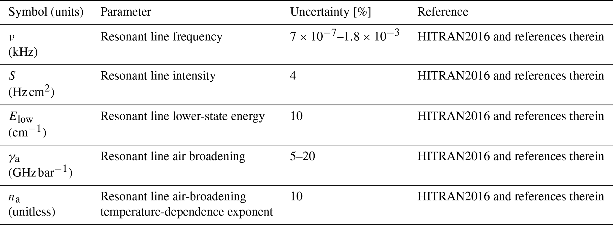
Figure 6 shows the $\mathrm{\Delta }{\mathit{T}}_{\mathrm{Bi},+}$ and $\mathrm{\Delta }{\mathit{T}}_{\mathrm{Bi},-}$ spectra corresponding to the perturbation to ozone line absorption parameters (ν, S, E_low, γ_a, n_a). The sensitivity analysis shows that among the model parameters in Table 3, which were perturbed by the estimated uncertainty, all of these impact the modeled upwelling 16–700 GHz T_B by more than 0.1 K.

However, we should emphasize that even though individual ozone lines contribute to the uncertainty by more than the chosen threshold, the contribution is rather small when averaged over finite channel bandwidths due to very narrow spectral line widths, as will be clarified in the next section. As a result, the ozone line parameters were not considered for evaluation of their covariance.

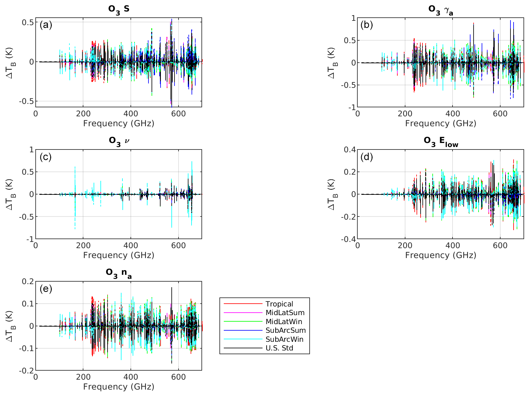
Figure 6 Sensitivity of modeled T_B to ozone line absorption and broadening parameters. Solid lines correspond to negative perturbation ($\mathrm{\Delta }{\mathit{T}}_{\mathrm{Bi},-}$) and dashed lines to positive perturbation ($\mathrm{\Delta }{\mathit{T}}_{\mathrm{Bi},+}$). Top: line absorption intensity (S) (a) and air-induced (b) broadening (γ_a) coefficients. Bottom: line frequency (ν) (c) and lower-state energy (E_low) (d). Temperature-dependence exponents of air-induced broadening (n_a) (e).

3 Channel convolution

The ultimate goal of this study is to characterize the absorption model uncertainty in simulated observations for selected satellite and airborne instruments, such as MWI, ICI, MWS, ATMS, MARSS, and ISMAR. Therefore, the spectral simulations, as well as the associated uncertainty, need to be convolved with the channel spectral response function, which is assumed to be a simple top-hat function in this context. Table 4 (Table 5) reports the list of MWI and ICI (MWS and ATMS) channels, with their associated characteristics. Hence, before proceeding with the covariance analysis of the identified dominant parameters, a further screening is performed to discard the parameters leading to perturbations that would give negligible contribution when convolved with channel spectral response function. In particular, spectrally narrow perturbations (delta-like) are likely to result in a negligible contribution when averaged within a channel bandwidth. As mentioned above, to simulate the channel convolution, here we consider a first-order approximation, i.e., a box average of the simulations falling within the channel bandwidth. Considering the spectral resolution used for the calculations (50 MHz, in addition to channels' central frequencies), the number of points falling within the bandwidths in Table 4 varies, reaching up to 100 for the largest bandwidth.

Table 4 List of MWI and ICI channels with the corresponding bandwidth.

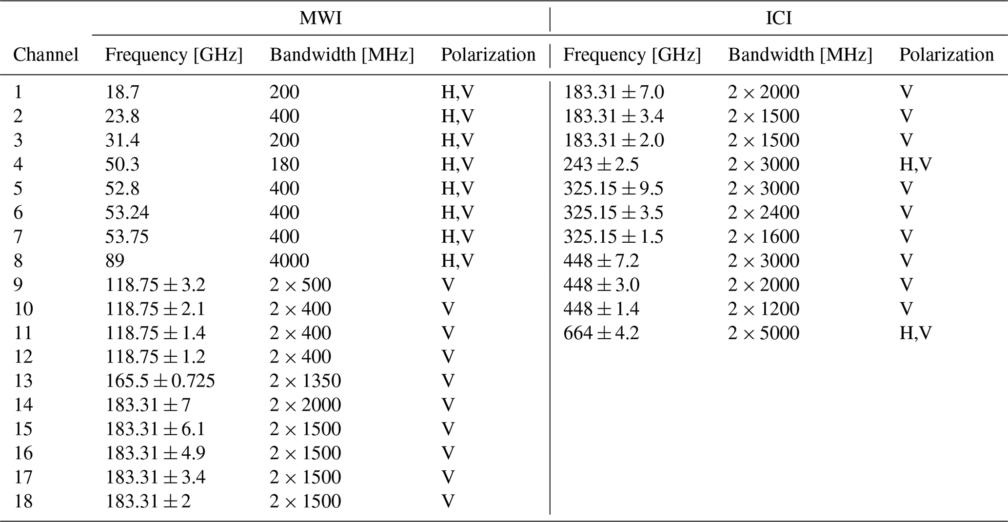
Note that the MWI channel 5 frequency was later changed to 52.7 GHz (with 180 MHz bandwidth) to avoid issues with radio frequency interference.

As seen in previous sections, delta-like spectrally narrow perturbations are associated with uncertainty in H₂O and O₂ central frequency ν, and all the five parameters considered for O₃ (ν, S, E_low, γ_a, n_a). The uncertainty in central frequency ν effectively locates the absorption peak within a narrow spectral range (∼100 kHz) around the absorption lines, leading to a very localized impulse going symmetrically from positive to negative. It should be noted that all double-sided channels in Table 4, except MWI channel 13, have a half bandwidth smaller than the detuning from the line center, with passbands at least 700 MHz away from any line center and thus far from the range impacted by the impulse. Similarly, MWI channel 13 is not affected by the impulse because it is located away from any resonant line absorption. In any case, although the perturbation can be large (of the order of 1 K or more), the average within a larger band would result in a negligible contribution. For these reasons, the uncertainty in central frequency ν is not further considered in the covariance analysis in Sect. 4. Similarly, it can be demonstrated that the perturbations related to the uncertainty in the five parameters considered for O₃ (ν, S, E_low, γ_a, n_a) have a negligible effect on the band-averaged simulations, i.e., less than 60 mK for any of the O₃ parameters.

4 Estimation of uncertainty covariance matrix

The sensitivity analysis from previous sections shows that the absorption model uncertainty in simulated upwelling T_B at finite-bandwidth channels is dominated by the uncertainty in 26 spectroscopic parameters for water vapor and 109 parameters for oxygen. For these parameters, the full covariance matrix of parameter uncertainties, including the off-diagonal terms giving the covariance of each parameter with the others, is required to compute the uncertainty in calculated T_B at any given frequency. The framework used to estimate the parameter covariance is described in Rosenkranz et al. (2018) and Cimini et al. (2018). Different methods are used to estimate covariance depending on how the parameter values were measured, but some general principles apply, as recapped hereafter. If a set of variables a_i have a causal dependence on another set of variables b_k,

$$\begin{array}{}\text{(5)}& \mathrm{\Delta }{a}_{\mathrm{i}}=\sum _{\mathrm{k}}(\partial a_{\mathrm{i}}/\partial b_{\mathrm{k}})\mathrm{\Delta }{b}_{\mathrm{k}},\end{array}$$

and if b has an uncertainty covariance matrix Cov(b), then

$$\begin{array}{}\text{(6)}& \mathrm{Cov}(a_{\mathrm{i}},b_{\mathrm{m}})=\sum _{\mathrm{k}}(\partial a_{\mathrm{i}}/\partial b_{\mathrm{k}})\mathrm{Cov}(b_{\mathrm{k}},b_{\mathrm{m}})\end{array}$$

and b contributes to the uncertainty covariance of a with the following amount:

$$\begin{array}{}\text{(7)}& \mathrm{\Delta }\mathrm{Cov}(a_{\mathrm{i}},a_{\mathrm{j}})=\sum _{\mathrm{m}}(\partial a_{\mathrm{j}}/\partial b_{\mathrm{m}})\mathrm{Cov}(a_{\mathrm{i}},b_{\mathrm{m}}).\end{array}$$

This general principle has been used to estimate the covariance between the selected 135 parameters. The full uncertainty covariance matrix Cov(p), as well as the correlation matrix Cor(p), for the set of 135 dominant spectroscopic parameters for water vapor and oxygen absorption is provided in the form of the Supplement along with the main paper. Further details are given in the following subsections.

Table 5 List of MWS and ATMS channels with the corresponding bandwidth.

4.1 Covariance of H₂O parameters

As described in Sect. 2.1, a total of 26 parameters were identified as dominant for H₂O absorption uncertainty, including continuum (C_s, C_f, $n_{{\mathrm{C}}_{\mathrm{s}}}$, $n_{{\mathrm{C}}_{\mathrm{f}}}$), and line (γ_a, n_a, S) parameters. In fact, water vapor contributes to absorption with several resonant lines and a non-resonant absorption, the latter being by definition the remainder after the contribution of local resonant lines has been subtracted from measured absorption. Therefore, if a line parameter is revised, the continuum should also be revised to compensate and reproduce as well as possible the original measurements from which the continuum was derived. Thus, line and continuum parameters are correlated. In addition, the self- and foreign-broadened continuum components are correlated, and so are their corresponding temperature-dependence exponents. The way covariance between C_s, C_f, $n_{{\mathrm{C}}_{\mathrm{s}}}$, and $n_{{\mathrm{C}}_{\mathrm{f}}}$ was derived is described in Cimini et al. (2018). The covariance between line intensities and continuum coefficients was derived in Rosenkranz et al. (2018), and it is here extended to higher-frequency lines (up to 916 GHz). The covariance between air-induced line widths and continuum coefficients was derived in Cimini et al. (2018), and it is here extended to the lines for which γ_a uncertainties were found to be relevant (i.e., the six H₂O key lines plus the 620 GHz line). The same approach was used to derive the covariance of line width temperature-dependence exponents with C_s and C_f.

On the other hand, if two parameters are derived independently, such as one by measurement and the other from theory, or by independent measurements, then we consider them uncorrelated. Thus (using the symbols defined in Table 1), $\mathrm{Cov}(S,n_{{\mathrm{C}}_{\mathrm{s}}})$, $\mathrm{Cov}(S,n_{{\mathrm{C}}_{\mathrm{f}}})$, Cov(S,γ_a), Cov(S,n_a), $\mathrm{Cov}({\mathit{\gamma }}_{\mathrm{a}},n_{{\mathrm{C}}_{\mathrm{s}}})$, $\mathrm{Cov}({\mathit{\gamma }}_{\mathrm{a}},n_{{\mathrm{C}}_{\mathrm{f}}})$, $\mathrm{Cov}(n_{\mathrm{a}},n_{{\mathrm{C}}_{\mathrm{s}}})$, $\mathrm{Cov}(n_{\mathrm{a}},n_{{\mathrm{C}}_{\mathrm{f}}})$, and (with one exception, which is discussed below) Cov(n_a,γ_a) are all set to zero.

The intensities of different absorption lines may be slightly correlated (∼0.1%) because of common assumptions in their theoretical calculations, but random deviation dominates (∼1%; Conway et al., 2018), and thus we set Cov(S_i,S_j) to 0 for i≠j.

The widths of different absorption lines and their temperature-dependence exponents were measured at low pressures such that they do not overlap and thus have independent uncertainties. Thus, $\mathrm{Cov}({\mathit{\gamma }}_{\mathrm{a},\mathrm{i}},{\mathit{\gamma }}_{\mathrm{a},\mathrm{j}})=\mathrm{Cov}(n_{\mathrm{a},\mathrm{i}},n_{\mathrm{a},\mathrm{j}})=\mathrm{0}$ for i≠j.

The exception noted above is at 325 GHz, where n_a comes from the measurements by Colmont et al. (1999), who derived γ_a and n_a as the intercept and slope of a linear fit between ln(γ_a) and ln(T). As such, the model to be fitted,

$$\begin{array}{}\text{(8)}& {\mathit{\gamma }}_{\mathrm{a}}\left(T\right)={\mathit{\gamma }}_{\mathrm{a}}\left(T_{\mathrm{0}}\right)(T_{\mathrm{0}}/T{)}^{{\mathrm{n}}_a},\end{array}$$

can be written as

$$\begin{array}{}\text{(9)}& y=a+bx,\end{array}$$

where

$$\begin{array}{}\text{(10)}& y=\ln \left({\mathit{\gamma }}_{\mathrm{a}}\right),a=\ln \left({\mathit{\gamma }}_{\mathrm{a}}\right(T_{\mathrm{0}}\left)\right),b=n_{\mathrm{a}},x=\ln (T_{\mathrm{0}}/T).\end{array}$$

The two parameters a and b are simultaneously fitted by least squares, so the reasoning in Cimini et al. (2018) (Sect. 4.1.3) applies. If the uncertainty in γ_a is small compared to its value, then the correlation between γ_a and n_a is

$$\begin{array}{}\text{(11)}& \mathit{\rho }({\mathit{\gamma }}_{\mathrm{a}},n_{\mathrm{a}})=\mathit{\rho }(a,b)=-<x>/\sqrt{{\mathit{\sigma }}_x^{\mathrm{2}}+<x{>}^{\mathrm{2}}},\end{array}$$

where $<x>$ is the average value of x and σ_x is its standard deviation.

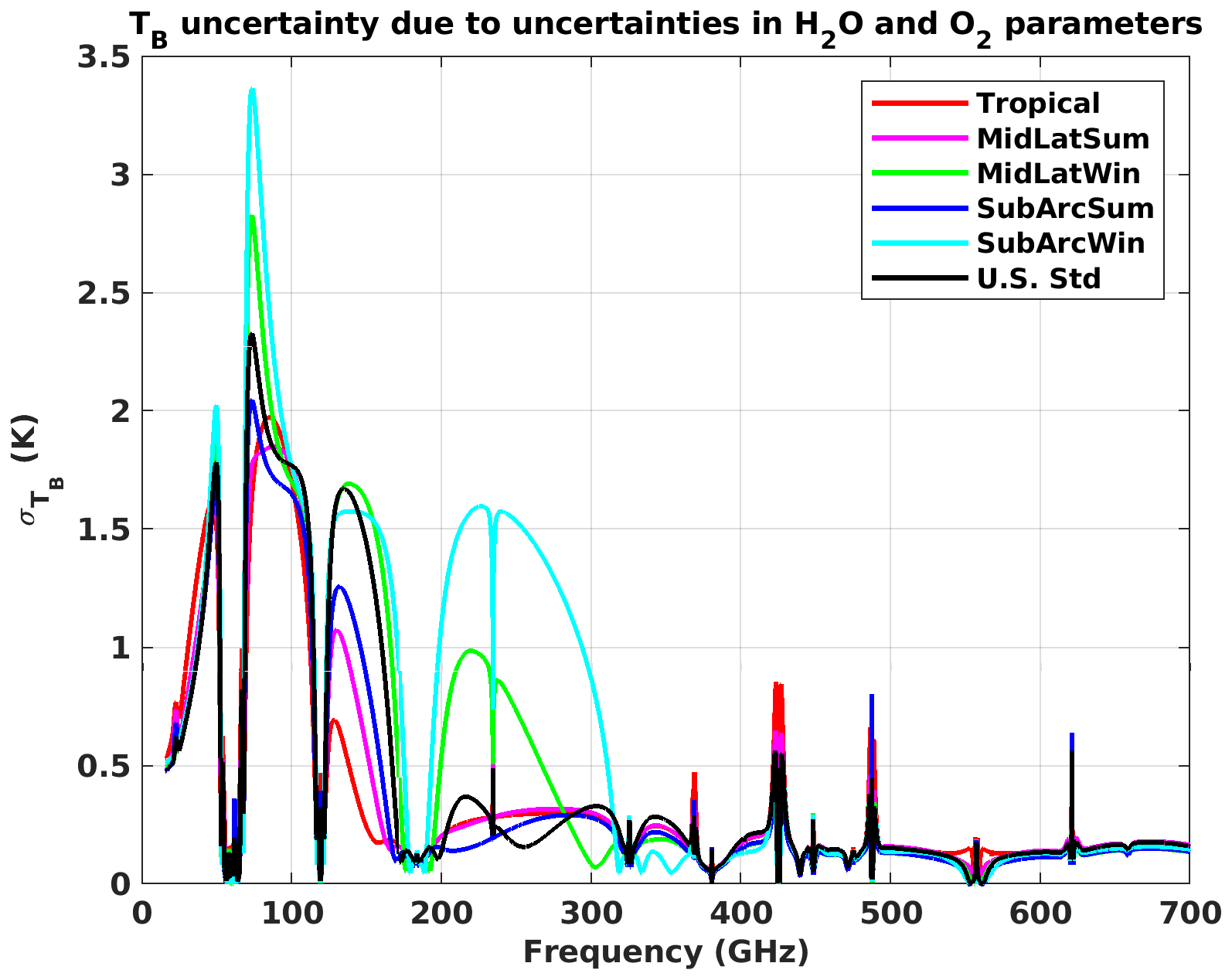
Figure 7 Brightness temperature uncertainty for downward-looking view at 53°, due to uncertainties in H₂O and O₂ parameters. Six typical climatology conditions are considered (tropical, midlatitude summer, midlatitude winter, sub-Arctic summer, sub-Arctic winter, US standard).

4.2 Covariance of O₂ parameters

As described in Sect. 2.2, 109 parameters were identified as dominant for O₂ absorption uncertainty, including zero-frequency continuum ($S_{\mathrm{0}}^{\prime }$, γ₀), line shape (S, γ_a, n_a), and line mixing (Y,V) parameters. Concerning the continuum absorption, it is very difficult to measure the broadening (γ₀) independently of the intensity ($S_{\mathrm{0}}^{\prime }$) for this zero-frequency pseudo-line. For that reason, Cimini et al. (2018) suggested that only the uncertainty in γ₀ could be used as a surrogate for the combination of $S_{\mathrm{0}}^{\prime }$ and γ₀. The estimated uncertainty is based on the spread of published measurements, accounting for the combination of intensity and broadening uncertainties. Concerning the line mixing (Y,V), only parameters for the first 34 lines (quantum number $N<\mathrm{33}+/-$) are included. The neglected lines, 15 in total, correspond to the 4 weakest lines of the 60 GHz band (50.9877, 68.4310, 50.4742, 68.9603 GHz), which are at least 1 order of magnitude weaker than the others, and 11 submillimeter lines, which are not significantly affected by line mixing at atmospheric pressures. Their contribution has been evaluated as negligible up to 20 % uncertainty in Y and V.

The covariance between the other parameters has been evaluated as in Cimini et al. (2018), with the following exceptions: in addition to the 34 lines above (quantum number $N<\mathrm{33}+/-$), the air-induced line widths (γ_a) of 4 submillimeter lines are also considered relevant, i.e., 234, 368, 424, and 487 GHz. These are assumed to be uncorrelated to other parameters as they are not affected by mixing and have been derived independently from intensity.

5 Uncertainty propagation to brightness temperature simulations

In the previous section the full uncertainty covariance matrix Cov(p) has been estimated for the set of 135 dominant parameters for water vapor and oxygen absorption. Thus, the full uncertainty covariance matrix for the computed T_B can be derived from Eq. (2), where K_p is the Jacobian of the radiative transfer model with respect to the spectroscopic parameters p and is computed by small-perturbation analysis. The next two sections present the results of the radiative transfer simulations, focusing firstly (Sect. 5.1) on the upwelling T_B, as seen from satellite sensors. Then Sect. 5.2 applies the above framework to upward-looking geometry.

5.1 Downward-looking view

The full T_B uncertainty covariance matrix corresponding to the lump contribution of the 135 dominant H₂O and O₂ spectroscopic parameters has been computed from Eq. (2) for the six typical climatology conditions introduced earlier (Anderson et al., 1986). Figure 7 shows the square root of the diagonal terms of each of the six T_B uncertainty covariance matrices, i.e., the T_B uncertainty spectra due to the 135 dominant H₂O and O₂ spectroscopic parameters for each of the six climatology conditions.

We notice that uncertainty in the millimeter-wave range is dominated by the water vapor continuum and the oxygen line mixing, with uncertainties in brightness temperature that reach up to 3.5 K. Conversely, in the submillimeter range the uncertainty due to water vapor absorption lines dominates the continuum absorption, as higher-frequency lines are very opaque and thus even the wings are stronger than the continuum absorption, which is relatively weaker in the middle to upper atmosphere, due to the quadratic dependence on water vapor pressure.

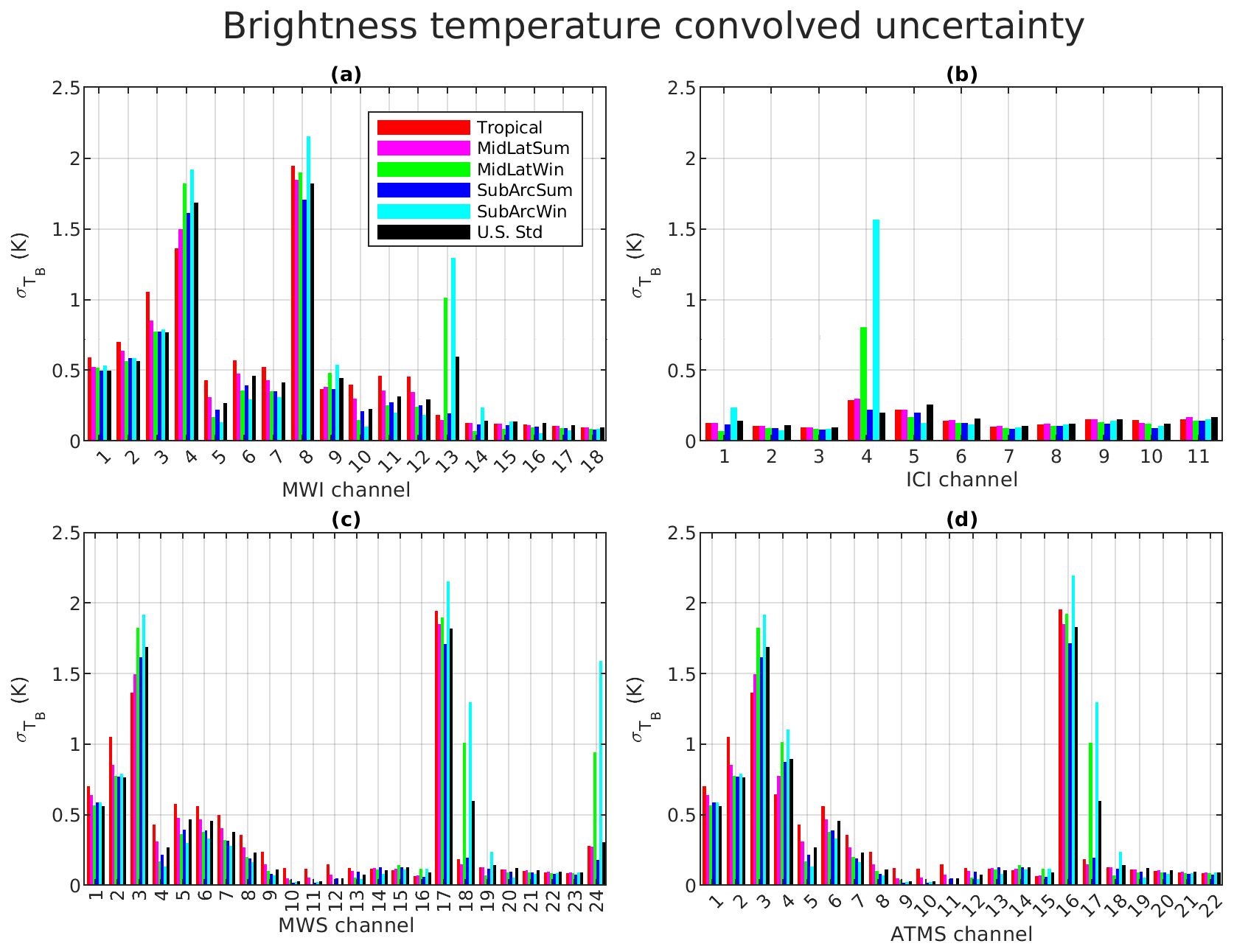
Figure 8 Brightness temperature uncertainty convolved on MWI and ICI (a, b) and MWS and ATMS (c, d) channels.

As previously mentioned, the major goal of this work is to provide uncertainties in synthetic T_B relative to channels of EPS-SG imagers and sounders. Hence we have performed the convolution of the spectra in Fig. 7 with top-hat functions corresponding to channel bandwidths reported in Tables 4 and 5 to estimate the corresponding uncertainty in simulated T_B for MWI, ICI, MWS, and ATMS. The results are shown in Fig. 8, with the uncertainty in simulated T_B computed for the six considered climatology conditions. It can be seen that generally the estimated uncertainty is not negligible and can reach more than 2 K. For ICI, the estimated uncertainty is quite small, less than 0.2 K, for all channels except channel 4, which has large uncertainty in cold and dry environments. MWS and ATMS sounders show very similar features, since they mostly have the same frequency channels: only a couple of channels show an uncertainty larger than 1 K, while the others feature smaller, though non-negligible, uncertainty values. These differences stem from different contributions from line and continuum absorption. This confirms that the uncertainty in brightness temperature simulations cannot be assumed to be negligible when comparing simulations with observations, such as within satellite sensor calibration and validation efforts, as they are of the same order as or even larger than typical radiometric accuracy (0.7–2.0 K for MWI and ICI).

5.2 Upward-looking view

While previous sections consider the downward-looking view from top of atmosphere (TOA), this section investigates the uncertainty associated with downwelling T_B, relative to the upward-looking geometry feasible with airborne sensors (e.g., Fox et al., 2024). Note that the same covariance matrix for 135 parameters is assumed here, while more rigorously the sensitivity should be reevaluated at each height. However, the 111 parameters that were selected in the previous study by Cimini et al. (2018) are included, although they were identified as dominant in the spectral range limited to 20–150 GHz. The six climatology conditions described earlier are used to compute the uncertainty covariance matrix corresponding to the lump contribution of the 135 dominant H₂O and O₂ spectroscopic parameters. But considering that airborne sensors typically change their altitude during the flight, the full T_B uncertainty covariance matrix has been computed assuming upward-looking zenith views from a set of nine altitudes (i.e., 0, 1, 2, 3, 5, 7, 8, 9, 10 km).

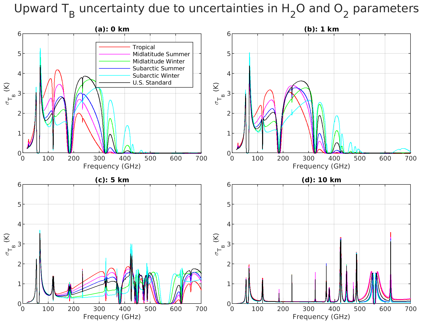
Figure 9 Brightness temperature uncertainty for the upward-looking view due to uncertainties in H₂O and O₂ parameters. Top: from 0 km (a) and 1 km (b) height; bottom: 5 km (c) and 10 km (d) height. Six typical climatology conditions are considered (tropical, midlatitude summer, midlatitude winter, sub-Arctic summer, sub-Arctic winter, US standard).

Figure 9 shows the square root of the diagonal terms of each resulting T_B uncertainty covariance matrix, i.e., the T_B uncertainty spectra due to the 135 dominant H₂O and O₂ spectroscopic parameters for each of the six climatology conditions. Four altitudes are shown, representative of observations from near the surface (0 km), within the boundary layer (1 km), the free troposphere (5 km), and the high troposphere (10 km). It can be seen that at low altitudes the uncertainty is dominated by water vapor continuum uncertainties (except for the 60 GHz band), while at high altitudes the uncertainty is dominated by line absorption uncertainties due to the different pressure dependencies of continuum (quadratic) and line (linear) absorption.

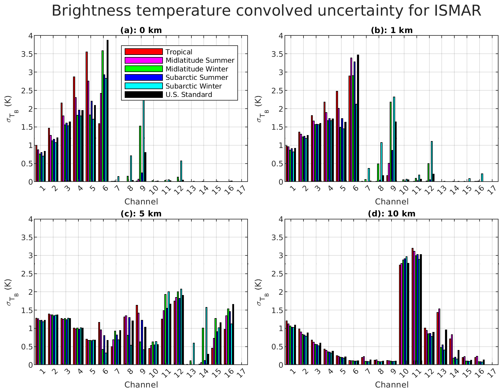
As done in Sect. 5.1 for the downward-looking geometry, the spectra in Fig. 9 can be convolved with the top-hat function corresponding to channel bandwidths in Table 6 to estimate the corresponding uncertainty in simulated downwelling T_B. This is performed only for ISMAR and MARSS channels, i.e., the two airborne instrument demonstrators considered in this study, since the upward-looking view from spaceborne sensors at TOA does not encounter the Earth's atmosphere. Accordingly, Figs. 10–11 show the uncertainty in simulated T_B for ISMAR and MARSS channels computed for the six considered climatology conditions from four representative altitudes: near the surface (0 km), within the boundary layer (1 km), the free troposphere (5 km), and the high troposphere (10 km). The resulting estimated uncertainty has been used in a companion paper to constrain observation-minus-simulation statistics collected in several airborne campaigns deploying ISMAR and MARSS (Fox et al., 2024).

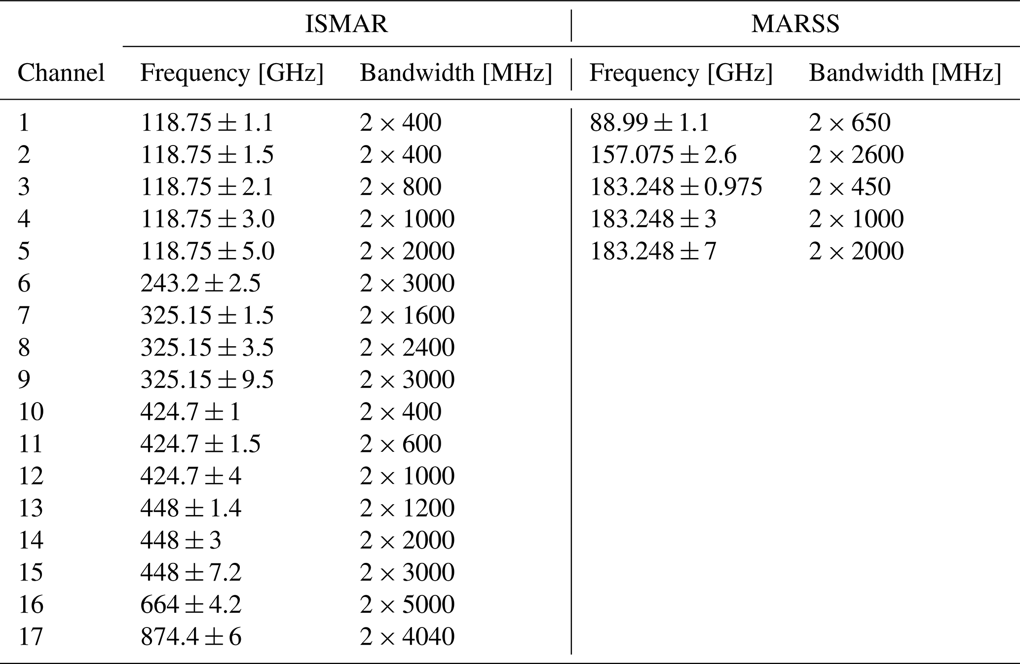
Table 6 List of ISMAR and MARSS channels with the corresponding bandwidth.

Figure 10 Brightness temperature uncertainty convolved on ISMAR channels (as in Table 6). ISMAR channel 17 is not shown as it lies outside of the frequency range considered in this study. Top: 0 (a) and 1 km (b) height; bottom: 5 (c) and 10 km (d) height.

6 Summary and conclusions

This paper quantifies the uncertainty in microwave radiative transfer calculations due to uncertainty in spectroscopic parameters in the framework of preparatory activity for the EPS-SG microwave radiometer. First, the sensitivity of radiative transfer calculations in the microwave–millimeter-wave range has been evaluated against the uncertainty in spectroscopic parameters for H₂O, O₂, and O₃, adopting the observing geometry typical of satellite imagers such as MWI and ICI (downward looking from TOA at a 53° incident angle) and surface emissivity for typical ocean conditions at H polarization, which is more conservative than V-pol for estimating the uncertainty related to the atmospheric absorption model. Note that uncertainties at a 53° incident angle could be assumed to be the higher boundary for cross-scanning instruments (such as MWS and ATMS), as the atmospheric path gets shorter at higher incident angles.

The sensitivity analysis identified a set of 135 spectroscopic parameters as dominant for the uncertainty in simulated T_B (26 for H₂O and 109 for O₂), while O₃ was judged to contribute only negligibly to the uncertainty in finite-bandwidth channels. The full uncertainty covariance matrix for the 135 spectroscopic parameters has been evaluated, including the off-diagonal terms indicating the cross-covariance between parameter uncertainties. Thus, the full T_B uncertainty covariance matrix, corresponding to the lump contribution of the 135 dominant H₂O and O₂ spectroscopic parameters, has been computed for six climatology conditions (tropical, midlatitude summer, midlatitude winter, sub-Arctic summer, sub-Arctic winter, US standard). Finally, the T_B uncertainty spectrum has been computed for each of the six different climatology conditions, as the square root of the diagonal terms of T_B uncertainty covariance matrices. The uncertainty in simulated T_B has also been evaluated for the MWI, ICI, MWS, and ATMS channels, considering their nominal bandpass filters, ranging from 0.1 K at relatively opaque channels to 2.2 K at relatively transparent channels (all numerical values are reported in Tables A1, A2, A3, and A4). These uncertainties are strictly valid over ocean surfaces (covering 72 % of the globe) and are deemed conservative with respect to other surface backgrounds, which usually have higher emissivity than the ocean. For example, the channel uncertainty has been evaluated using typical sea-ice emissivity, showing lower values throughout the spectral domain and especially at lower frequency (10–100 GHz) for which sea-ice emissivity gets closer to 1. The channel uncertainty was also quantified for two airborne instruments (ISMAR and MARSS) assuming zenith upward-looking observations at different aircraft altitudes (0–10 km), showing values from just above 0.0 to 3.8 K, depending on the channel opacity and assumed climatology.

The analysis above was obtained using PWR19. Therefore, the quantified uncertainties are strictly valid for this model. The uncertainty in other absorption models, adopting a different spectroscopy, could be evaluated with the same approach. One relevant absorption model is that developed and maintained by AER, Inc. (Clough et al., 2005; Cady-Pereira et al., 2020) adopting the MT_CKD water vapor continuum model (Mlawer et al., 2019, 2012), as it was used to train the ICI coefficients for the fast RTMs adopted for the ICI operational retrievals and data assimilation in NWP models (RTTOV version 13). Considerations of the characteristics of the AER and MT_CKD model, with respect to PWR19, indicate that uncertainty in the H₂O continuum would decrease by half due to smaller continuum coefficients’ uncertainty (by roughly 50 %, Eli Mlawer, personal communication, 2021; although the difference is more complex as highlighted by Odintsova et al., 2017), while the uncertainty deviation due to H₂O line absorption would be small (<0.1 K) except in the 20–25 GHz range (∼ 0.8 K increase).

Figure 11 As in Fig. 10 but for MARSS channels in Table 6.

The uncertainty due to O₂ parameters is expected to be the same, as PWR and AER models share the same O₂ spectroscopic parameters from Tretyakov et al. (2005). However, such a speculative analysis is limited by the fact that the MT_CKD formulation is more complicated – i.e., the parameters vary with frequency and wavenumber – and that we were not able to find information concerning the correlation between MT_CKD continuum coefficients and the way O₂ line mixing parameters and their temperature dependence are used within the AER code.

Finally, while this analysis was being finalized, an updated spectroscopy was released (PWR22, available at http://cetemps.aquila.infn.it/mwrnet/lblmrt_ns.html, last access: 10 June 2024; Rosenkranz, 2019). Appendix B reports expected systematic and random differences between PWR22 and PWR19; this gives an indication of the additional uncertainty in PWR19 with respect to the latest version, which includes more millimeter-wave water vapor lines and more recent spectroscopic findings, while an extension of the uncertainty analysis to PWR22 is planned as future work.

Appendix A: Uncertainty values

In this section we report the values for top-of-atmosphere upwelling brightness temperature uncertainty (at 1σ level) arising from the uncertainty covariance of 135 spectroscopic parameters identified as dominant (109 related to O₂ absorption, 26 related to H₂O absorption) for channels of the MicroWave Imager (Table A1), Ice Cloud Imager (Table A2), MicroWave Sounder (Table A3), and Advanced Technology Microwave Sounder (Table A4). The convolution with a top-hat response function, taking into account a channel bandwidth, is computed for both horizontal and vertical polarization, for each of the six climatology atmospheric profiles. We also show in Fig. A1 a graphical representation of the full covariance matrix of T_b uncertainties for MWI, ICI, MWS, and ATMS, relative to horizontal polarization and US standard climatology (see the Supplement for other climatologies and vertical polarization).

Table A1 Uncertainty for simulated TOA upwelling T_B [K] at MWI channels [GHz] due to uncertainties in H₂O and O₂ parameters. Six climatological atmospheric conditions are considered: tropical, midlatitude summer (MidLatSum), midlatitude winter (MidLatWin), sub-Arctic summer (SubArcSum), sub-Arctic winter (SubArcWin), and US standard (US std.).

Table A2 As in Table A1 but for ICI.

Table A3 As in Table A1 but for MWS.

Table A4 As in Table A1 but for ATMS.

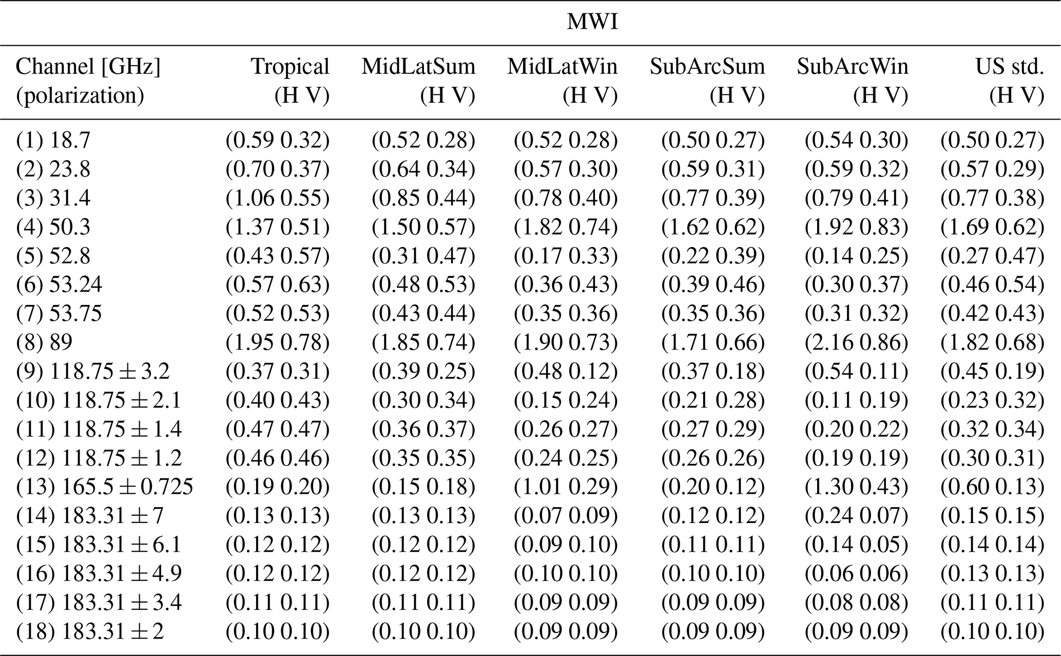
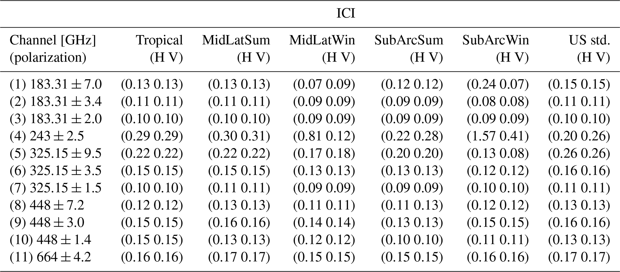
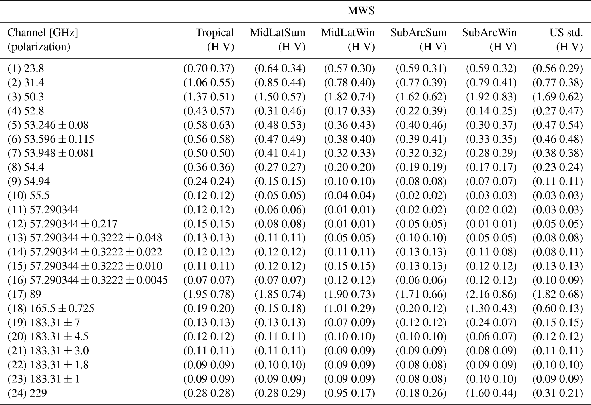
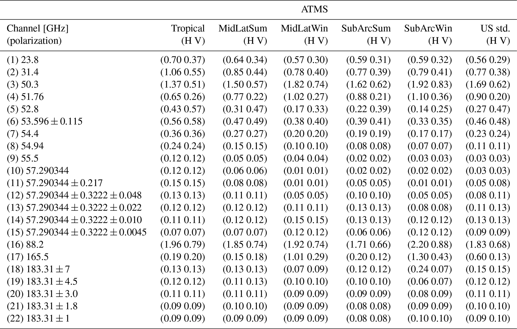
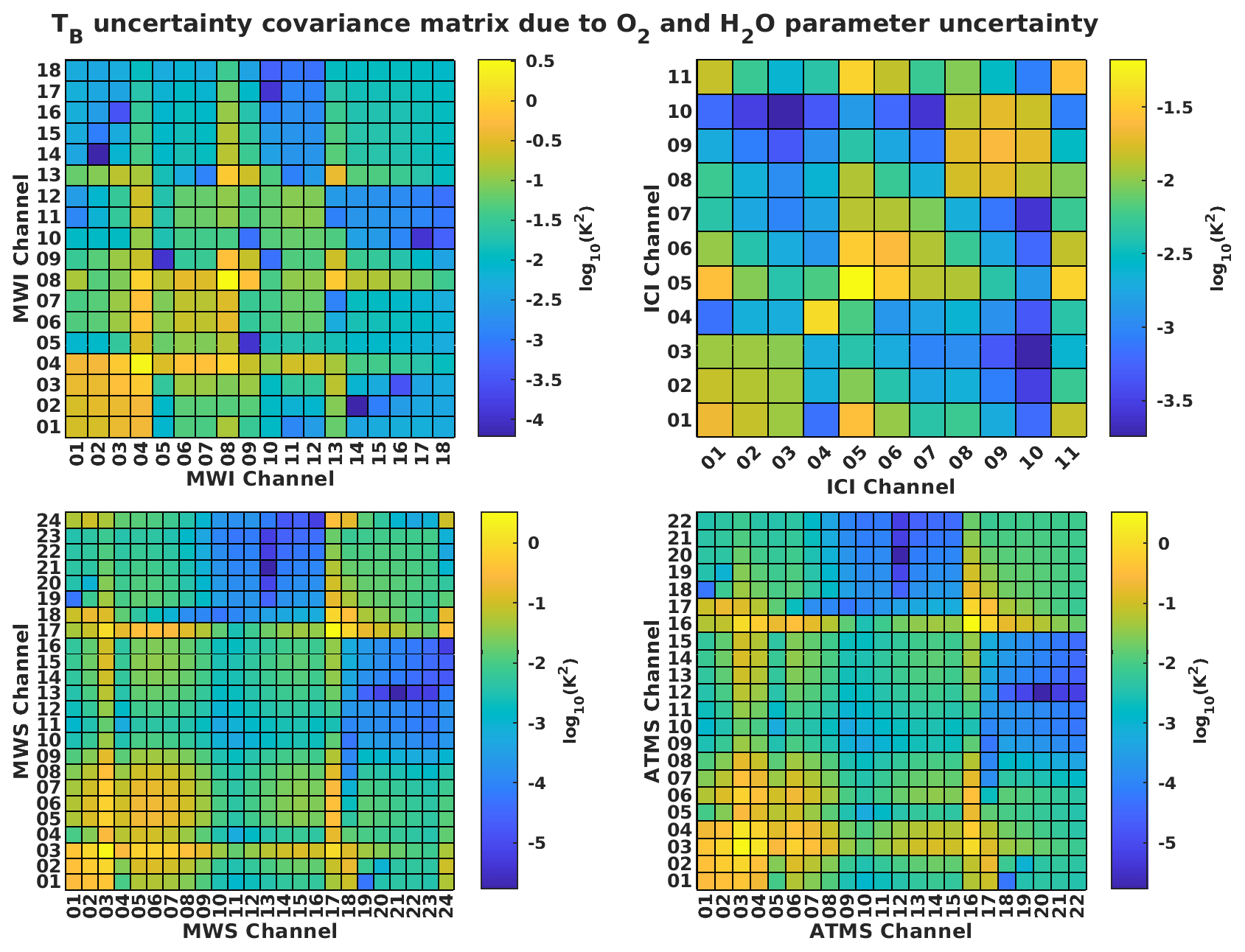
Figure A1 T_B uncertainty covariance matrix due to O₂ and H₂O absorption model parameter uncertainty for MWI, ICI, MWS, and ATMS in the case of horizontal polarization and US standard climatology. Numbers in the figure are in kelvins squared (K²), while the color scale is in log₁₀(K²). Note that for graphical reasons, the figure shows the absolute values of the covariance.

Appendix B: Expected differences between PWR19 and PWR22

Spectroscopic parameters are continuously investigated, with their values and uncertainty being updated. With respect to PWR19 used here, values for several parameters have been updated in the PWR release of January 2022 (PWR22, available at http://cetemps.aquila.infn.it/mwrnet/lblmrt_ns.html, last access: 10 June 2024; Rosenkranz, 2019). Differences between T_B computed with PWR22 and PWR19 in the 10–800 GHz range (50 MHz resolution) are reported in Fig. B1 for the six typical climatology conditions (tropical, midlatitude summer, midlatitude winter, sub-Arctic summer, sub-Arctic winter, US standard). The most significant differences with respect to PWR19 are (i) in the 50–70 GHz range and around 118 GHz, due to the update of O₂ line-coupling parameters, which now include second-order line mixing (Makarov et al., 2020); (ii) around 183 GHz for the introduction of speed-dependent line shape at this water vapor line (Koshelev et al., 2021); (iii) above 600 GHz for the inclusion of four water vapor lines (860, 970, 987, 1097 GHz); and (iv) for updating line parameters taken from HITRAN according to the latest release available (HITRAN2020) (e.g., O₂ 16O18O isotopologue line at 234 GHz).

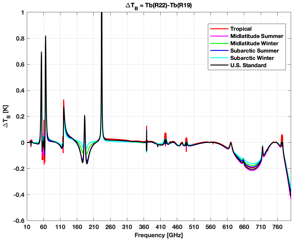
Figure B1 Differences between brightness temperature computed using PWR22 and PWR19 absorption models (PWR22 minus PWR19). Six typical climatology conditions are considered (tropical, midlatitude summer, midlatitude winter, sub-Arctic summer, sub-Arctic winter, US standard).

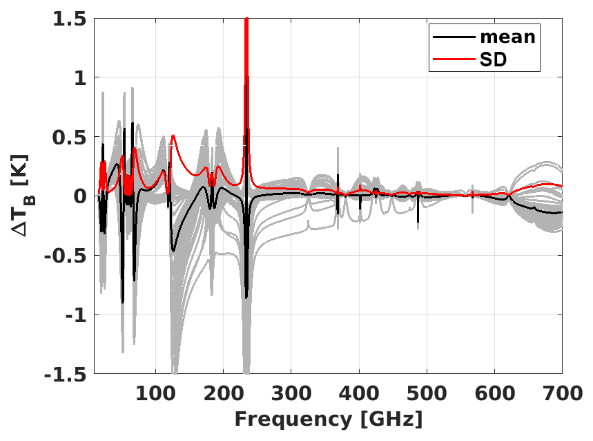
Figure B2 Brightness temperature difference (PWR22 minus PWR19) using 83 diverse profiles (grey lines) and their mean (black) and SD (red). The y axis is limited to ±1.5 K, but the SD at 234 GHz exceeds 10 K.

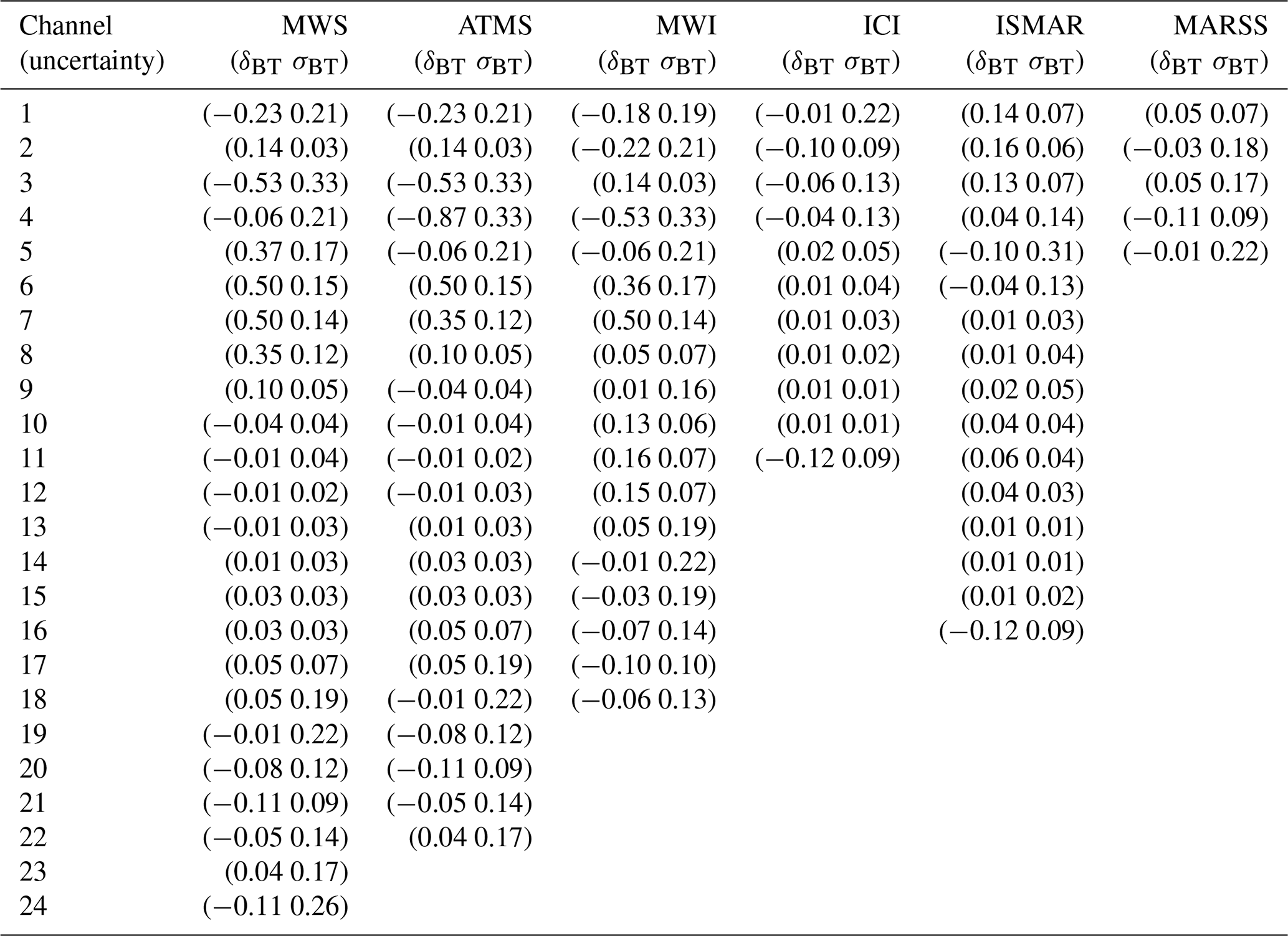
Assuming PWR22 as the reference for the most updated spectroscopy, additional uncertainty could be associated with the PWR19 calculations as the typical systematic and random difference with respect to PWR22. These differences have been investigated through a set of diverse atmospheric profiles. The set of 83 atmospheric profiles was selected to represent the diverse range of possible atmospheric conditions (Matricardi, 2008), and it is commonly used to train the regression coefficients in RTTOV (Saunders et al., 2018). It has also been used extensively in Turner et al. (2022) (e.g., their Appendix A). The spectral difference between PWR22 and PWR19 using the diverse profiles, as well as their mean and SD, is shown in Fig. B2. Note that the SD difference spectrum stays within the uncertainty calculated for PWR19 (see Fig. 7), and thus it is consistent with that. The only feature for which the SD difference is larger than the PWR19 uncertainty is at 234 GHz, related to the O₂ 16O18O isotopologue line, for which the strength was lowered by a factor of 4 starting from HITRAN2016 on. Note that the only channels that are affected are ICI channel 4 (234 GHz) and MWS channel 24 (229 GHz), with an impact not larger than 0.13–0.26 K, as can be seen from Table B1, where the convolutions of mean and SD difference spectra on instrument channels are reported.

Table B1 Estimated additional systematic and random uncertainty associated with PWR19 calculations, taking the latest model release as reference (PWR22).