the Creative Commons Attribution 4.0 License.
the Creative Commons Attribution 4.0 License.
 | 21 Jun 2024
On the uncertainty of anthropogenic aromatic volatile organic compound emissions: model evaluation and sensitivity analysis
Marc Guevara
Oriol Jorba
Hervé Petetin
Dene Bowdalo
Carles Tena
Gilbert Montané Pinto
Franco López
Carlos Pérez García-Pando
Volatile organic compounds (VOCs) significantly impact air quality and atmospheric chemistry, influencing ozone formation and secondary organic aerosol production. Despite their importance, the uncertainties associated with representing VOCs in atmospheric emission inventories are considerable. This work presents a spatiotemporal assessment and evaluation of benzene, toluene, and xylene (BTX) emissions and concentrations in Spain by combining bottom-up emissions, air quality modelling techniques, and ground-based observations. The emissions produced by High-Elective Resolution Modelling Emission System (HERMESv3) were used as input to the Multiscale Online Nonhydrostatic AtmospheRe CHemistry (MONARCH) chemical transport model to simulate surface concentrations across Spain. Comparing modelled and observed levels revealed uncertainty in the anthropogenic emissions, which were further explored through sensitivity tests. The largest levels of observed benzene and xylene were found in industrial sites near coke ovens, refineries, and car manufacturing facilities, where the modelling results show large underestimations. Official emissions reported for these facilities were replaced by alternative estimates, resulting in varied improvements in the model's performance across different stations. However, uncertainties associated with industrial emission processes persist, emphasising the need for further refinement. For toluene, consistent overestimations in background stations were mainly related to uncertainties in the spatial disaggregation of emissions from industrial-use solvent activities, mainly wood paint applications. Observed benzene levels in Barcelona's urban traffic areas were 5 times larger than the ones observed in Madrid. MONARCH failed to reproduce the observed gradient between the two cities due to uncertainties arising from estimating emissions from motorcycles and mopeds, as well as from different measurement methods and the model's capacity to accurately simulate meteorological conditions. Our results are constrained by the spatial and temporal coverage of available BTX observations, posing a key challenge in evaluating the spatial distribution of modelled levels and associated emissions.
- Article
(12073 KB) - Full-text XML
- BibTeX
- EndNote


Volatile organic compounds (VOCs) significantly contribute to air pollution and pose serious health hazards to humans. These compounds originate from diverse sources, resulting from anthropogenic and biogenic activities (Kansal, 2009). They can also be produced by the oxidation of other VOCs, with this secondary formation being predominant for some VOCs (e.g. formaldehyde) (Parrish et al., 2012; Luecken et al., 2012). Anthropogenic sources include various human-driven activities, such as solvent use, traffic and fuel evaporation, and industrial emissions, as well as residential biomass burning (Monks et al., 2015; Kansal, 2009). Within urban areas, VOC emissions are predominantly influenced by human activities, with vehicular emissions representing over 60 % of VOCs in European urban areas (Borbon et al., 2018). Meanwhile, biogenic VOCs (BVOCs) also play a crucial role in atmospheric chemistry. Globally, BVOCs represent a larger fraction of total VOCs and exhibit higher chemical reactivity compared to many anthropogenic VOCs (Guenther et al., 2006). Additionally, it is important to note that human-induced atmospheric changes, driven by emissions from sources like industrial processes, transportation, and agriculture, increase oxidant levels, which can also boost natural aerosol production like biogenic secondary organic aerosol (SOA; Kanakidou et al., 2000).
One essential aspect of VOCs is their contribution to tropospheric chemistry, as they are major precursors for ozone (O3) (Atkinson and Arey, 2003; Carter, 1990) and/or secondary organic aerosol (SOA) formation (Chen et al., 2022; Ziemann and Atkinson, 2012). In Spain, for specific areas and conditions, VOCs contribute to high-O3-concentration episodes (In't Veld et al., 2024; Querol et al., 2017, 2018; Castell et al., 2008). For example, in Barcelona, In't Veld et al. (2024) estimated that anthropogenic VOCs were significant contributors to O3 formation, accounting for 38 % and 49 % of the measured ozone formation potential (OFP) during winter and summer, respectively. Also, Oliveira et al. (2023) showed that in Spain, toluene and xylene are in the top 5 main species contributing to OFP, while benzene, although having a low reactivity, is in the top 20 species contributing to OFP. Moreover, they play a key role in the formation of SOA (Baltensperger et al., 2005; Cui et al., 2022; Sun et al., 2016; Jookjantra et al., 2022), which significantly contributes to fine particulate matter (PM2.5) (Srivastava et al., 2022; Zhang et al., 2019; Ziemann and Atkinson, 2012). Huang et al. (2014) found that SOA contributes about 30 % to 77 % of PM2.5 mass concentrations in their study, which focused on severe haze pollution events in specific urban areas.
While some VOCs may not be associated with acute health impacts, they can still lead to chronic health risks (Shuai et al., 2018; Alford and Kumar, 2021). Notably, aromatic compounds, such as benzene, toluene, and xylene (commonly referred to as BTX), are of particular concern (Filley et al., 2004; Tagiyeva and Sheikh, 2014; Niaz et al., 2015; Ling et al., 2023), with benzene being classified as a group A carcinogenic compound by the US Environmental Protection Agency (Bayliss et al., 1998). This study focuses on BTX because (1) they are continuously measured over time in various locations, providing an important temporal and spatial coverage; (2) they represent a substantial part of the total anthropogenic emissions – more than 20 % at the global scale according to Yan et al. (2019) and possibly more in urban areas (Bates et al., 2021); and (3) they are important precursors of O3 and SOA.
Within the air quality modelling chain, the emission inventories, while being a significant source of uncertainty, serve as key elements to understand air pollution origins, in forecasting applications, and to design effective emission abatement strategies (Russell and Dennis, 2000; Day et al., 2019). Despite the importance of VOCs, as previously stated, among all the air pollutants reported by emission inventories (e.g. NOx, SOx, CO, NH3, PM10, PM2.5), VOCs are typically associated with the highest emission uncertainty. For example, in Spain, when considering the combined uncertainty of both emission factors (EFs) and activity data, VOC emissions show uncertainties between 15.6 % and 490 % across the different sectors, which is more than for other species, such as for NOx emissions which report uncertainties between 3.6 % and 175 % (MITERD, 2022). This is mainly due to limited efforts in updating the EFs and limited information on the activity data of some key sectors (e.g. use of solvents).
Chemical transport models (CTMs) are a powerful tool for assessing and forecasting atmospheric pollutant concentrations (EC, 2008). They support the design of effective air quality (AQ) control strategies by assessing the potential impacts of specific emission reduction scenarios (Agency, 2011). When evaluated against observed pollutant concentrations, they typically provide key insights on the validity of emission inventories, even with overlapping uncertainties arising from various sources across the entire evaluation chain. These uncertainties include those related to emissions, the capability of the CTM to accurately reproduce chemical and meteorological conditions, and a wide range of uncertainties in observational data (i.e. the measurement technique, instrumentation). CTMs are most commonly evaluated on the main criteria pollutants for which more observations are available (Badia and Jorba, 2015; Georgiou et al., 2022; Skoulidou et al., 2021), but an important gap persists on the VOCs (She et al., 2023). As an example, Air Quality Expert Group (2020) recently highlighted the absence of model–observation evaluations of VOCs over the UK. This identified gap is due to several reasons: first, the models use simplified chemical mechanisms. These mechanisms group the numerous individual VOC species into broader families based on known reactions or the number of carbon bonds they possess (e.g. the Carbon Bond 2005 chemical mechanism, CB05; Yarwood et al., 2005). This grouping enables the models to accurately replicate O3–NOx chemistry with both acceptable precision and computational efficiency. This limitation not only restricts the number of species that can be individually evaluated against observations but also impacts the model's accuracy in representing them. Second, emission inventories report total VOCs, which then requires the need to use speciation profiles which are limited and commonly outdated (Oliveira et al., 2023). Third, the availability and quality of observational data for VOCs are often limited in scope (von Schneidemesser et al., 2023; She et al., 2023). Typically, continuous measurements of VOCs prioritise aromatics due to the recognised health risks associated with their exposure. Despite the EU's AQ directive (AQD) recommending the measurement of 31 VOC species, only benzene is currently regulated (EC, 2008). As for other VOCs, the measurements usually come from small campaigns which are limited in time and location (von Schneidemesser et al., 2023).
This study aims to quantify limitations and uncertainties in Spanish anthropogenic BTX emissions and to improve its representation in air quality modelling systems. To do so, we used the High-Elective Resolution Modelling Emission System (HERMESv3; Guevara et al., 2019b, 2020) model to produce gridded bottom-up emissions, which were used as input in the Multiscale Online Nonhydrostatic AtmospheRe CHemistry (MONARCH; Badia et al., 2017; Klose et al., 2021a) chemical transport model to simulate surface concentrations of benzene, toluene, and xylene (i.e. o-, m-, and p-xylene) across Spain. The modelling results were then evaluated against official ground-based observation data for the year 2019. By conducting this evaluation, we are able to identify the spatio-temporal characteristics of the observed concentrations, quantify the differences with modelled results, and link these divergences to uncertainties in the emissions used as input through a set of sensitivity analyses.
2.1 Model description
2.1.1 HERMESv3
HERMESv3 (Guevara et al., 2019b, 2020) is an open-source, parallel, and standalone multi-scale atmospheric emission modelling framework that computes anthropogenic emissions for atmospheric-chemistry models. The model consists of two modules, a global–regional module (HERMESv3_GR) and a bottom-up module (HERMESv3_BU), that can work combined or separated depending on the working domain and scope of the applications. For this work, the HERMESv3_GR module is only used to process emissions reported by the Copernicus Atmospheric Monitoring Service (CAMS) regional gridded inventory (CAMS-REGv4.2; Kuenen et al., 2022) outside of Spain as well as for the shipping sector, while the HERMESv3_BU is used to produce bottom-up anthropogenic emissions in Spain (Guevara et al., 2020).
The HERMESv3_BU module estimates anthropogenic emissions at high spatial (e.g. road link, industrial facility level) and temporal (hourly) resolution using state-of-the-art calculation methods, based on (but not limited to) the calculation methodologies reported by the European EMEP/EEA air pollutant emission inventory guidebook, which combine local activity and emission factors. Specifically for this work, the model resolution was set to feed MONARCH at a spatial resolution of 0.1° by 0.1°. The model computes bottom-up emissions from energy and manufacturing industrial facilities, road transport, residential and commercial combustion activities, other mobile sources (landing and take-off cycles in airports, agricultural machinery, recreational boats, shipping emissions in ports), fugitive emissions from fossil fuels (storage and transportation), domestic and industrial use of solvents, and agricultural activities (livestock and use of fertilisers).
The industrial emissions at the plant level used in HERMESv3 are derived from the national large point source (LPS) database and from the Spanish Pollutant Release and Transfer Register (PRTR-Spain). Both databases are compiled and maintained by the Spanish Ministry for the Ecological Transition and the Demographic Challenge (Ministerio para la Transición Ecológica y el Reto Demográfico, MITERD), which estimates the emissions using the information provided by the corresponding industrial facilities (MITERD, 2023, 2022). Priority is given to the LPS database when both datasets provide values for the same facility, since the data reported by the LPS database are consistent with the official inventories.
The VOC speciation mapping disaggregates total VOCs to the species needed by the atmospheric-chemistry model of interest and its corresponding gas-phase and aerosol chemical mechanism. Each individual sector is assigned with a set of profiles with numerical factors (mole of chemical species per gram of source pollutant) to convert the total emissions into the output model species. The number of speciation profiles considered varies according to the pollutant sector of interest. For instance, in the case of residential combustion, the number of speciation profiles proposed is equal to the number of fuel types considered (e.g. natural gas, biomass). In contrast, in the case of road transport, specific profiles are assigned to each vehicle category (Guevara et al., 2020). The speciation profiles used in HERMESv3 are based on the work done by Oliveira et al. (2023), which performed a collection, review, and comparison of profiles available from recent studies.
2.1.2 MONARCH
The MONARCH model (Badia et al., 2017; Klose et al., 2021a) is an online multipurpose atmospheric-chemistry integrated system. MONARCH includes a gas-phase module combined with a hybrid sectional-bulk multi-component mass-based aerosol module to simulate the chemistry of the troposphere. MONARCH is coupled online with the Nonhydrostatic Multiscale Model on the B grid (NMMB; Janjic and Gall, 2012) meteorological core. A detailed evaluation of MONARCH in reproducing different meteorological parameters, such as temperature, relative humidity, wind speed, wind direction, radiation, and planetary boundary layer (PBL), is described elsewhere (Brunner et al., 2015; Sicard et al., 2021).
The gas-phase chemistry in MONARCH solves the Carbon Bond 2005 chemical mechanism (CB05; Yarwood et al., 2005) extended with chlorine chemistry (Sarwar et al., 2012) and additional oxidation pathways to form SOA from benzene, toluene, xylene, isoprene, and terpenes. Benzene is implemented to form SOA, while xylene and toluene are also involved in O3–NOx chemistry. The reactions solved by the model involving BTX are shown in Appendix A. The core CB05 mechanism considers 51 chemical species and solves 156 reactions. VOCs are lumped into several groups, such as propionaldehyde and higher aldehydes (ALDX), acetaldehyde (ALD2), ethene (ETH), formaldehyde (FORM), internal olefin (IOLE), terminal olefin carbon bond (OLE), paraffin carbon bond (PAR), terpene (TERP), toluene and other monoalkyl aromatics (TOL), and xylene and other polyalkyl aromatics (XYL). Notably, the mechanism also accounts for explicit species, namely benzene (BENZENE), ethane (ETHA), ethanol (ETOH), isoprene (ISOP), and methanol (MEOH).
The CB05 is well formulated for various tropospheric conditions, from urban to remote areas. It employs the Fast-J scheme to calculate photolysis rates (Wild et al., 2000), which considers the influence of clouds, aerosols, and absorbers such as ozone. The dry deposition of gases uses a resistance scheme based on Wesely (1989) for the canopy or surface resistance, while scavenging and wet deposition for precipitating and non-precipitating clouds follows the scheme of Byun and Ching (1999); Foley et al. (2010). Further details (i.e. aerosol processes) are available elsewhere (Spada, 2015; Klose et al., 2021a; Navarro-Barboza et al., 2023).
For this work, MONARCH was set up with a rotated latitude–longitude projection, with a spatial resolution of 0.1° by 0.1° for Spain. The domain over Spain is presented in Fig. 1. The setup accounts for 24 vertical layers (top 50 hPa). The boundary conditions for the meteorological module come from the European Centre for Medium-Range Weather Forecasts (ECMWF) Reanalysis v5 (ERA5) for the year of 2019, and the chemistry is derived from the CAMS global atmospheric composition reanalyses, which is built on ECMWF's Integrated Forecasting System (IFS; Flemming et al., 2015). We chose to focus on the year 2019, as the emissions and observational data for 2022 had not been validated at the time of our analysis, and the use of emission data from 2021 or 2020 would be significantly affected by the COVID-19 pandemic (Guevara et al., 2023).
As previously mentioned, the anthropogenic emissions are fed by HERMESv3. The biogenic emissions are estimated with MEGANv2.04 (Guenther et al., 2006, 2012), which is fully implemented inside MONARCH. The speciation employed emits xylene (lumping p-cymene and o-cymene MEGAN species) and toluene (lumping toluene, benzaldehyde, methyl benzoate, phenylacetaldehyde, methyl salicylate, and indole MEGAN species) among other biogenic species.
2.2 Air quality network and observational data
In order to evaluate the performance of the MONARCH model, we used the data obtained for the year 2019 from the European Environment Agency (EEA) AQ e-reporting (EEA, 2023) and complemented with data provided by the Spanish ministry (MITERD, 2020). To do so, we used the harmonised dataset from Globally Harmonised Observations in Space and Time (GHOST). The GHOST dataset is one of the most extensive collections of harmonised measurements of atmospheric composition at the surface level. More detailed information can be found in Bowdalo et al. (2024). From this dataset, our selection process only considered observations that meet the default quality assurance (QA) criteria specified by GHOST (the details of the QA applied can be found in Table C1 of the Appendix C) and have temporal coverage greater than 75 % in 2019. When applying these filters, 62 stations measuring benzene were dropped, along with 10 stations measuring toluene and 6 stations measuring xylene. The removal of these stations caused a reduction of spatial coverage, where the majority of the stations were located in the south and north-western part of Spain. The temporal coverage criteria were the main driver to remove these stations, although the QA criteria number 83 (see Appendix C for the full description) also had a substantial impact. This shows, mainly for stations measuring benzene, the low quality of the measurements available, and while this reduction may be perceived as a limitation for model evaluation, it is a critical measure to ensure the reliability of measurements. It is also crucial to recognise the potential measurement uncertainties, as exemplified by Gallego-Díez et al. (2016), which can significantly vary based on the chosen methodology and instrumentation setup. The measurement methods for each station, when available, are detailed in Appendix H.
Table 1Available number of stations in Spain by area classification and station type measuring benzene, toluene, and xylene in 2019 after applying a temporal coverage of 75 % and quality assurance criteria. The number of stations that only measure with daily resolution is shown in parentheses.
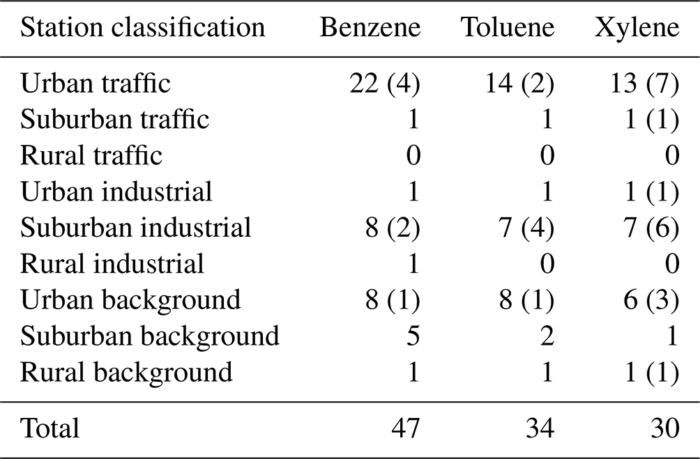
Table 1 shows the available number of stations in Spain per station classification measuring benzene, toluene, and xylene in 2019. The locations and spatial distribution of the stations, along with their respective classifications, are shown in Fig. 1. Examining the spatial distribution of the final dataset reveals a heterogeneous coverage. Notably, there is a lack of monitoring stations in the southern and north-western regions of Spain, as well as in Barcelona, specifically for stations measuring toluene and xylene. A complete description of the location, area, and station classification as well as the measuring time resolution of each station can be found in Appendix H.
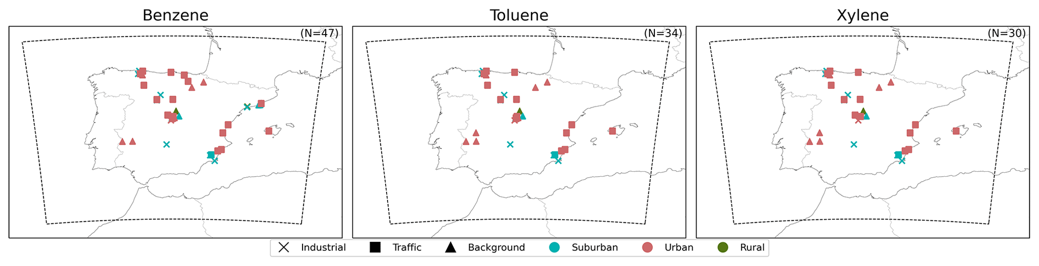
Figure 1Location of the air quality stations measuring benzene, toluene, and xylene (with a temporal coverage over 75 % and filtered by the QA criteria) by type and area classification in Spain for 2019. The station classification is represented by distinct markers, while the area classification is indicated by varying colours. The characteristics of each station are listed in Appendix H.
3.1 Emissions
Figure 2 shows the total anthropogenic emissions of benzene, toluene, and xylene in Spain per grid cell (4 km by 4 km) for the year 2019. The analysis of the emission results excludes the estimated MEGAN biogenic emissions, as it does not report any emissions for benzene, and their contribution to total toluene and xylene was found to be minimal (Henrot et al., 2017). To support the discussion, a map identifying the name and location of the different Spanish NUTS2 (Nomenclature of Territorial Units for Statistics) administrative regions and the main cities mentioned in this work is provided in Fig. B1 in Appendix B.
The total estimated emissions in Spain are 11 kt (kilotons) for benzene, 26 kt for toluene, and 12 kt for xylene. The main Spanish NUTS2 administrative regions emitting benzene are Andalusia (1.7 kt, 17 % of the total emitted benzene), Aragon (1.6 kt, 15 %), and Catalonia (1.4 kt, 14 %). Notably, each NUTS2 region exhibits distinct emission characteristics. In Andalusia, the residential sector accounts for the majority of emissions, contributing 74 % (1.3 kt), primarily from wood combustion. In contrast, for Aragon and Catalonia, the industrial sector is the main source of emissions, comprising 82 % (1.3 kt) and 53 % (0.8 kt), respectively. Aragon's substantial industrial contribution is primarily due to the presence of a large paper and pulp manufacturing industry, which is responsible for 40 % of industrial benzene emissions in this region.
For toluene emissions, the top-emitting NUTS2 regions are Catalonia (6 kt, 23 % of the total emitted toluene), the Valencian Community (3 kt, 11 %), and Andalusia (3 kt, 11 %). Similarly, in the case of xylene, the top emitters are Catalonia (2.1 kt, 19 % of the total emitted xylene), Andalusia (1.4 kt, 12 %), and the Valencian Community (1.3 kt, 11 %). For both pollutants, the solvent sector predominates, accounting for 72 % and 89 % of total emissions, respectively. In Andalusia, the solvent sector contributes less to xylene emissions (50 %) due to the presence of several petrochemical complexes, which account for approximately 25 % of these emissions. It is worth noting that Madrid has significant emissions, with 2.5 kt of toluene and 1.2 kt of xylene. However, due to its smaller area compared to other regions, it does not rank in the top 3. Nevertheless, when looking at the emission intensity, Madrid ranks first for toluene (emitting 0.31 t km−2) and xylene (emitting 0.15 t km−2) and second for benzene (emitting 0.06 t km−2).
Overall, regions with higher emission values in Spain tend to coincide with more populated areas or significant industrial activity. For instance, regions with the lowest population density (about 26 inhabitants per square kilometre), namely Castile and León, Castile–La Mancha, and Extremadura (INE, 2021), despite collectively covering 44 % of peninsular Spain's total area, contribute only 15 %, 14 %, and 13 % of total benzene, toluene, and xylene emissions, respectively. Regarding spatial distribution, benzene hotspots are located in specific industrial areas, such as Toledo in the south of Madrid and Tarragona in the south of Catalonia. In contrast, hotspots for toluene and xylene are primarily located in urban areas.
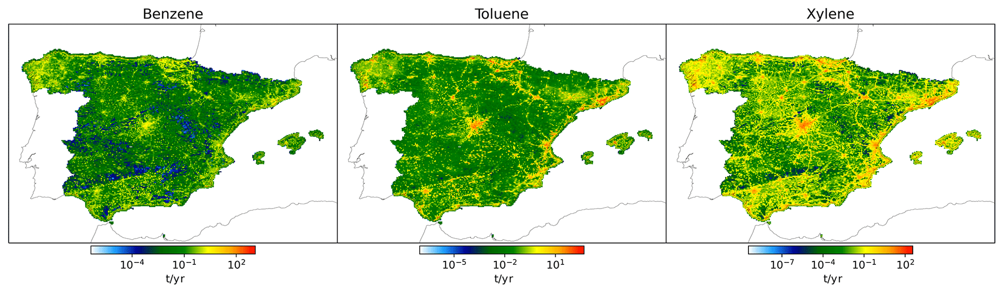
Figure 2Bottom-up estimated emissions (t yr−1) of benzene, toluene, and xylene in Spain at 4 km by 4 km.
To quantify the contribution of the different anthropogenic activities to total BTX emissions, we conducted individual runs of HERMESv3_BU, grouping its emission sectors as follows: (1) road transport; (2) the solvent sector was divided depending on its application, resulting in domestic use and industrial, which accounts for the solvent production and use in the industrial context; (3) residential, which corresponds to the residential and commercial combustion sector; (4) industry, which accounts for energy and manufacturing industrial emissions except for VOC process emissions linked to the use of solvents (e.g. manufacturing of chemical products or paint application); and (5) other, which accounts for the remaining emission sectors, including, aviation (landing and take-off cycles in airports), shipping in port areas, recreational boats, livestock, agricultural machinery, and the fugitive fossil fuel sector.
Figure 3 shows the contribution for each grouped sector per day over the year of 2019 and VOC species for urban areas in Spain. The information regarding urban settlements was sourced from Schiavina et al. (2023). Benzene emissions show notable variations throughout the year, with industries being the primary contributor, accounting for 35 % to 44 % on average. Another relevant source is the road transport, which contributes on average 29 %. However, due to the weekday–weekend effect, the contribution from this sector decreases during weekends. It is worth mentioning that the emissions from the residential sector show a big seasonality, as they are primarily driven by the burning of wood for residential heating. While the contribution is higher in more rural areas, decreases from 18 % in winter to 6 % in summer (figure not included).
The contribution of the different sources to toluene emissions remains quite constant along the year, with the industrial solvent sector being the primary contributor, averaging around 85 % annually. Within the industrial solvent sector, the primary activities emitting toluene are the fabrication and treatment of chemical products, such as paint manufacturing (50 %), industrial paint application (14 %), and non-industrial paint application (10 %). The domestic use of solvent, despite having an important contribution to total VOCs (around 11 % in 2019), has a very limited contribution to BTX emissions compared to industrial use of solvent because the speciation profile used assumes less than 1 % for each individual species.
Similar to toluene, xylene is also primarily dominated by the solvent sector, with a contribution averaging around 77 % annually. Overall, the shares show a relatively constant pattern, where road transport contributes from 10 to 16 %, reaching higher values in winter. For xylene, the main activity from the industrial solvent sector is the paint application, such as industrial paint application (41 %), wood paint application (16 %), and paint application in the manufacturing of automobiles (11 %).
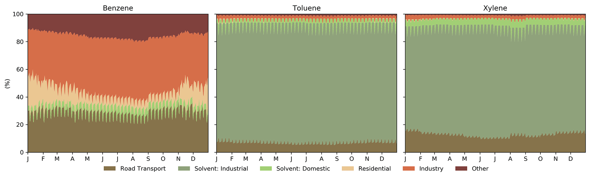
Figure 3Temporal source contribution (%) to total emissions of benzene, toluene, and xylene in Spanish urban areas in 2019.
Figure 4 shows the contribution (%) of each sector to total benzene, toluene, and xylene emissions per grid cell at a resolution of 4 km by 4 km. A similar figure is presented in Appendix D showing the emissions (t) of benzene, toluene, and xylene by emission sector. For benzene, the residential sector is the dominant sector in Spain, with an overall contribution of over 86 %, except in urban areas, where the contribution is generally under 20 %. This is more evident in Madrid and Barcelona, although it can be seen in all major cities. This spatial pattern can be attributed to the predominant emission of benzene from residential biomass combustion, which in HERMESv3 is allocated based on rural population density due to the minimal usage of this fuel in urban areas, where natural gas dominates the energy mix. In urban areas, the main contribution comes from the road transport sector (overall, over 60 %) and to a smaller extent from the domestic solvent use (up to 24 %). As expected, over major interurban roads, the road transport sector is usually the main contributor. In the more rural areas, agriculture activity dominates benzene emissions, contributing around 94 %. Furthermore, the industrial sector makes a substantial contribution (> 90 %) to specific grid cells, particularly in areas where large facilities and industrial hotspots are situated. This is mostly evident over the Catalonia region but also over main industrial areas such as Valencia and the central region of Andalusia.
For toluene and xylene, the contribution by sectors shows a similar spatial pattern. The industrial solvent sector dominates the urban areas with overall values ranging between 63 %–97 %. However, the cells intersecting main interurban roads are dominated by the traffic sector, contributing around 44 %–80 %. The residential emissions have an essential contribution in more rural areas, mainly due to biomass burning, where they are more relevant for xylene (up to 76 %) than for toluene (up to 70 %). The main differences between toluene and xylene spatial patterns are seen for “other”. Despite having lower values (see Fig. 2), rural areas are predominantly characterised by livestock emissions, primarily from cattle. In several locations, grid cells are entirely dominated by the livestock sector. The variations in cattle emissions between toluene and xylene can be attributed to the differences in their respective speciation, with toluene accounting for a greater percentage (1 %) than xylene (< 0.1 %) (Oliveira et al., 2023).
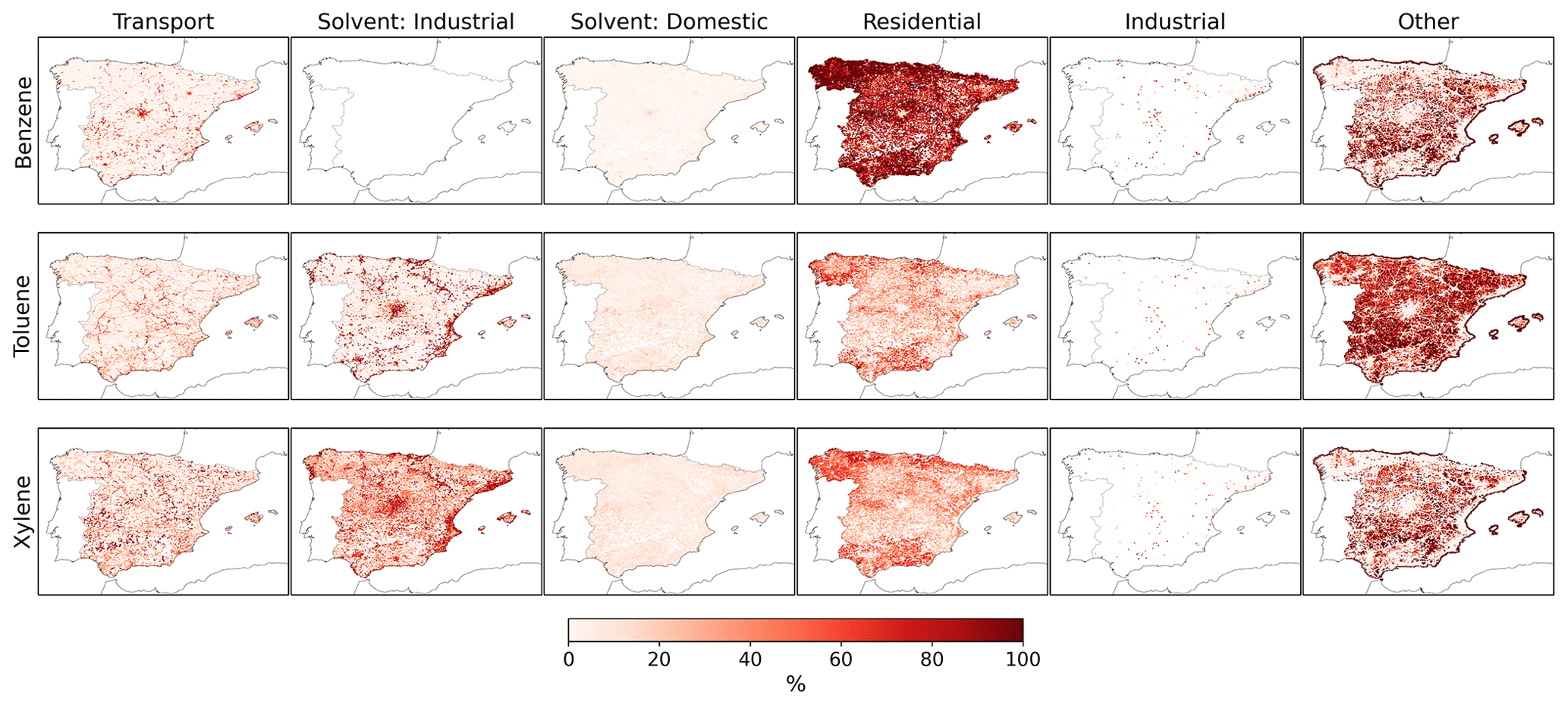
Figure 4Relative contribution (%) of individual anthropogenic emission sources to total benzene, toluene, and xylene annual emissions in Spain in 2019 per grid cell (4 km by 4 km).
3.2 Surface BTX concentrations
The following subsection presents the comparison between modelled BTX concentrations estimated with MONARCH and observations reported by air quality stations. Additionally, an evaluation of NO2 and O3 is presented in Appendix F to support the analysis. To match explicit toluene and xylene observations, we assumed that ratios between explicit and lumped species from emissions could be extrapolated to concentrations. Spatially (gridded and per type of station) and temporally (monthly) resolved ratios (i.e., toluene/TOL and xylene/XYL) were estimated using HERMESv3 and the speciation information reported by Oliveira et al. (2023) and applied to the model outputs (see Appendix G). On average in Spain, for TOL total mass, toluene contribution is 63 %, while for XYL total mass, (m, o, p)-xylene contribution is 41 %.
The location and characteristics of each specific station are presented in Appendix H. To analyse the impact of the different emission sectors and reduce the number of variables, we evaluated the model by aggregating the measurement stations by station type and area classification as follows.
-
Urban and suburban traffic stations were aggregated because of observed trend similarities. Although the model has limitations in replicating traffic sites accurately, analysing these sites can still yield valuable information.
-
All industrial stations were aggregated due to their similar observed range values and trends.
-
Urban and suburban background stations were aggregated due to their similar observed trends, and this consolidation was necessary given the limited availability of suburban background stations measuring toluene (N=2) and xylene (N=1). Rural background stations were excluded from the analysis as only one site with these characteristics was available.
Annual and seasonal mean statistics are computed for each group of stations, with seasons corresponding to winter (January, February, and December), spring (March, April, and May), summer (June, July, and August), and autumn (September, October, and November). The statistics used in this work are commonly used to evaluate model performances against observations. For this, we selected N (sample size), observed mean, modelled mean, mean bias (MB), normalised mean bias (NMB), root mean squared error (RMSE), and the Pearson correlation coefficient (r).
Figure 5 shows the annual mean concentrations of (a) benzene, (b) toluene, and (c) xylene for the year 2019, modelled with a spatial resolution of 0.1° by 0.1° and observed at various air quality stations. The detailed discussion for each pollutant is provided along the section.
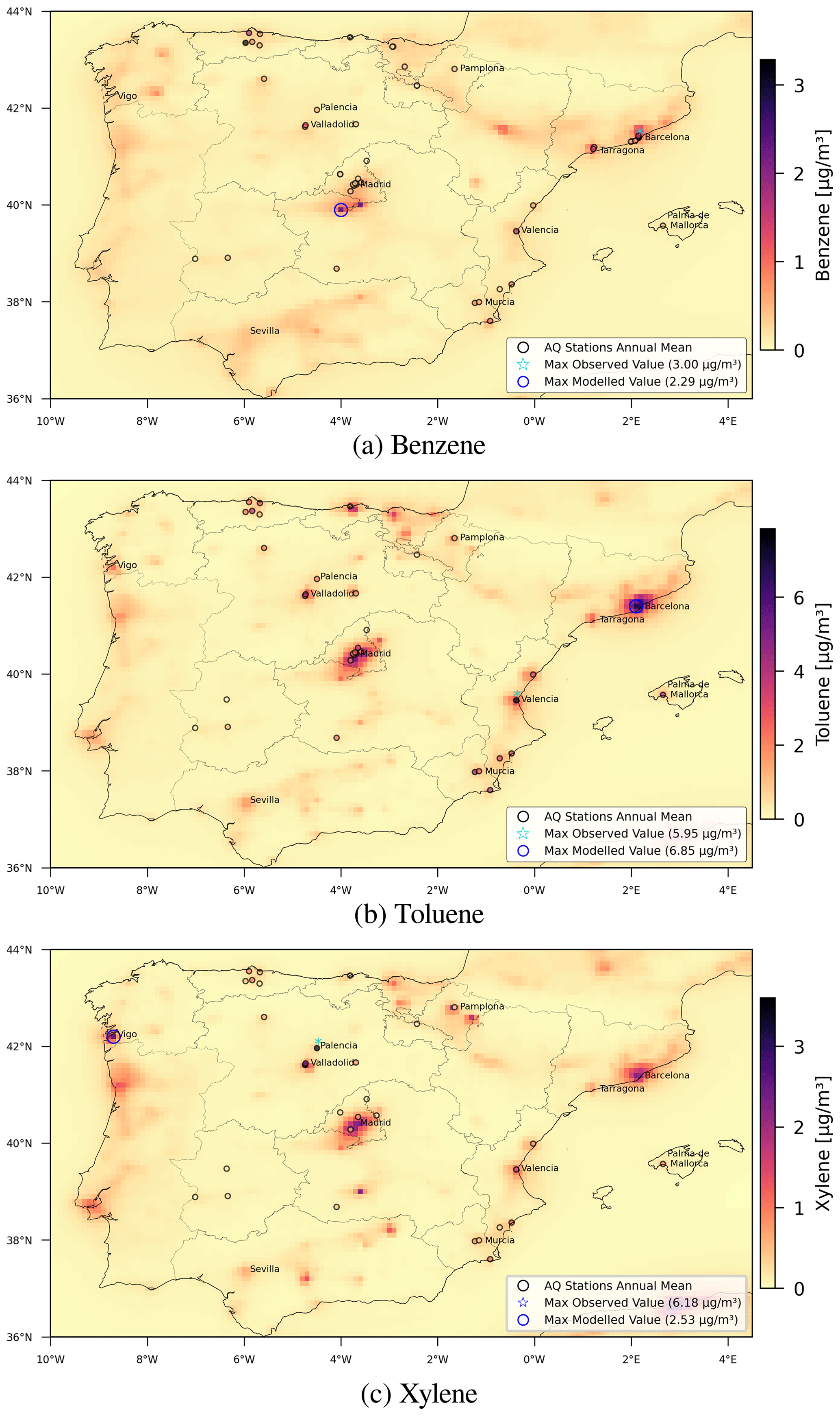
Figure 5Annual mean of modelled (0.1° by 0.1°) and observed concentrations (µg m−3) for 2019 for (a) benzene, (b) toluene, and (c) xylene. Black circles represent air quality station locations, while colours represent the annual mean observed values. The star indicates the station with the highest observed value, and the blue circle marks the maximum modelled value.
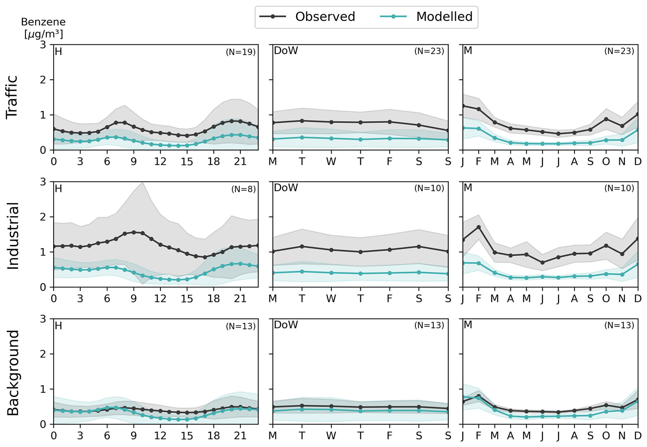
Figure 6Observed (black line) and modelled (blue line) benzene hourly (H), weekly (day of the week, DoW), and monthly (M) cycles (µg m−3) per station classification. The shaded region corresponds to the standard deviation variability.
3.2.1 Benzene
As previously mentioned, benzene is the only compound currently regulated in the EU by the AQD, with a limit value of 5 µg m−3 (annual mean). Air quality monitoring stations in Spain consistently report values below this regulatory limit, and none record levels near the limit. Notably, the highest recorded benzene concentration is observed in Barcelona at a traffic station (ES1438A, 3.00 µg m−3), followed by an industrial station in Asturias near facilities with coke ovens (ES2075A, 2.89 µg m−3), and another Barcelona urban traffic station (ES1480A, 2.59 µg m−3). The World Health Organization (WHO) also establishes a reference level (RL) of 1.7 µg m−3 for the annual mean concentration of benzene (WHO, 2019), which is surpassed only by the three monitoring stations mentioned above, underscoring the overall compliance with the air quality standards but not completely for the health guidelines.
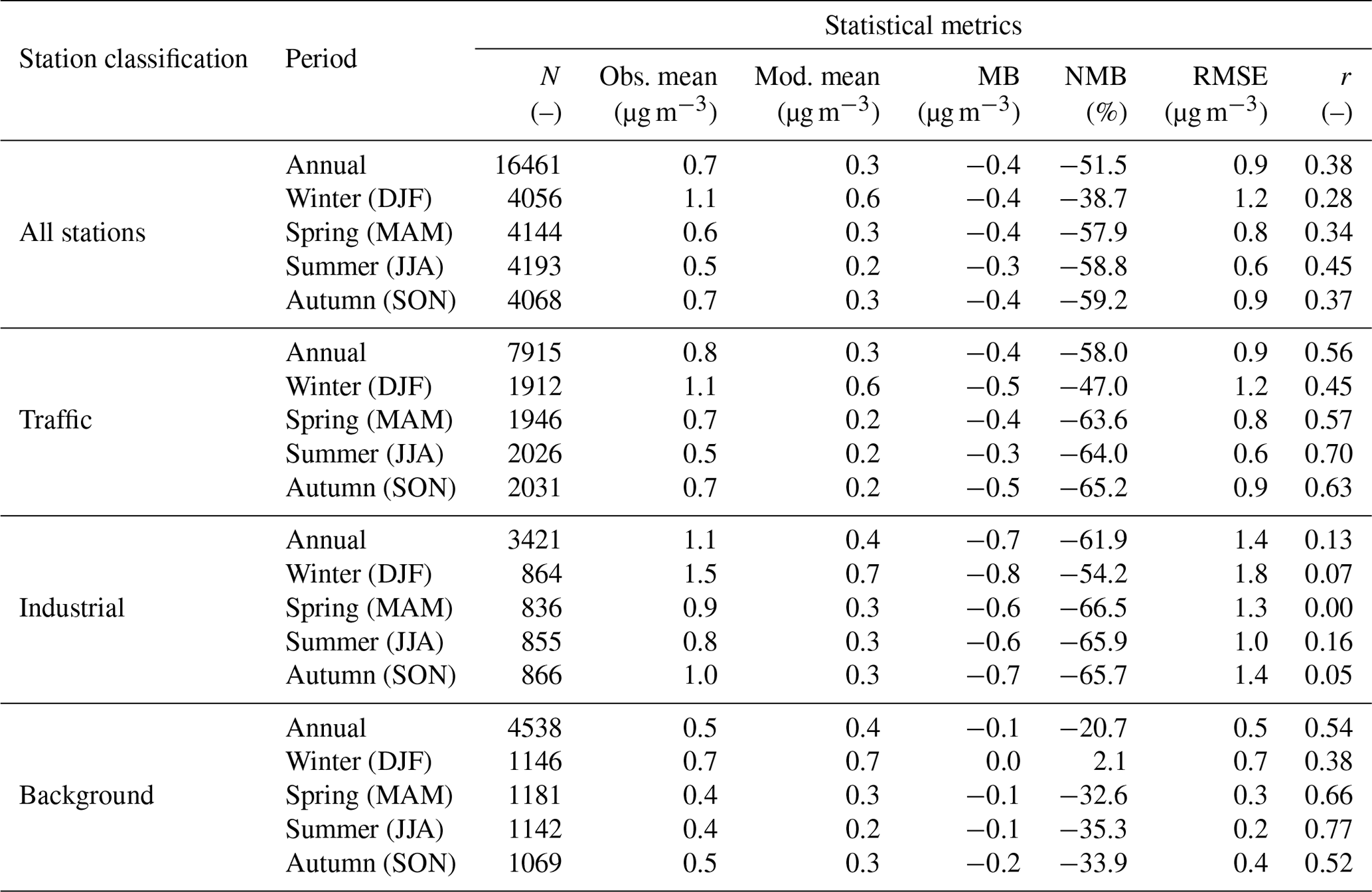
Table 2Seasonal and annual statistics for N, observed mean, modelled mean, MB, NMB, RMSE, and r per station classification for benzene for Spain in 2019 obtained with MONARCH.
The spatial distribution of annual mean benzene concentrations in both observed and modelled data shows a fairly consistent alignment (see Fig. 5a). However, the model struggles to replicate isolated hotspots, primarily attributable to its resolution and the sporadic occurrence of high peaks (mainly in industrial areas), which, using classical emission inventory approaches, is challenging to reproduce. The maximum annual mean value modelled by MONARCH is 2.29 µg m−3, also below the AQD limit value, and located south of Madrid, very close to two chemical facilities, namely one that produces chemical organic and inorganic products and another that produces pharmaceutical chemical products. Unfortunately, no stations are located in this area to validate the modelled results.
In general, as depicted in Fig. 5a (also supported by Fig. E1a in Appendix E), the model tends to underestimate benzene concentrations. The MB is generally low for the urban stations, from −0.21 to 0.92 µg m−3 (NMB between −67 % and 56 %), showing an adequate model performance in these areas. However, the model tends to be highly underestimated for some specific stations where the largest concentrations are observed. This is mainly attributed to underestimations of VOC emissions. Although, to a lesser extent, the model's coarse resolution could also limit its capacity to accurately capture intense urban and industrial hotspots. It is worth nothing that the resolution plays a smaller role since the models perform well in replicating NO2 concentrations in industrial areas (see Appendix F). The largest underestimations are mainly observed in the east coast, particularly in Barcelona, at two traffic stations, ES1438A (MB = −2.17 µg m−3 and NMB = −72.3 %) and ES1480A (MB = −1.75 µg m−3 and NMB = −67.4 %), as well as one traffic station in the Valencian Community (ES1239A, MB = −1.26 µg m−3 and NMB = −76.2 %). The same happens for suburban stations measuring high concentration levels, which occur in the northern part of the country in Asturias. For instance, industrial station ES2075A (MB = 1.21 µg m−3 and NMB = −93.0 %) is located near two coke oven facilities, and industrial station ES0879A (MB = −2.69 µg m−3 and NMB = −80.5 %) is located near one coke oven facility. Of the 13 suburban stations, 8 are near major industrial facilities like refineries and coke ovens, showing larger underestimations. The suburban stations located in Madrid and Barcelona in background environments show low MB values (−0.24 to 0.54 µg m−3).
Figure 6 shows the comparison between observed and modelled hourly, daily, and monthly benzene cycles per station classification, including the variability of the standard deviation as the shaded region. Table 2 provides statistical metrics for all stations and by station classification, both for the entire year and for each season, including N, observed mean, modelled mean, MB, NMB, RMSE, and r.
Observed benzene levels show marked seasonal variations, with the highest levels occurring during winter across all stations, a characteristic that is also captured by MONARCH. Correlation coefficients (r) vary by season, with the highest value observed in summer (0.45) and the lowest in winter (0.28). The annual NMB indicates that, on average, the model underestimates benzene levels by approximately −51.5 %. This underestimation is more pronounced in industrial stations (−61.9 %) and much less in background stations (−20.7 %). The NMB is also heterogeneous across seasons, with winter being the period in which the underestimation is at the lowest level (−38.7 % for all stations) when compared to the other seasons (e.g. −59.2 % in autumn). The model slightly overestimates levels during winter at background stations, where the NMB is 2.1 %. Background stations generally exhibit lower underestimations and higher correlation coefficients, suggesting a better model performance in this type of environment. This is also observed in the comparison between modelled and observed background hourly, monthly, and weekly cycles, with results indicating generally good performance of MONARCH, except for the small overestimation of the morning peak.
The model consistently underestimates benzene levels in traffic stations (MB = −0.4 µg m−3 and NMB = −58 %) while effectively replicating the observed hourly, monthly, and weekly cycles. These underestimations can be partially attributed to the model's resolution (i.e. approximately 10×10 km2), as this can lead to a “smoothing” of emissions and subsequently result in underestimations of concentrations in these stations. Nevertheless, the performance of the model is not consistent across urban traffic sites. While in Madrid the model exhibits a good performance and low MB values (between −0.20 and 0.14 µg m−3), in other large cities like Barcelona and Valencia, the model's underestimations are more significant (see Fig. E1a), indicating a potential misrepresentation of local sources that are characteristic of these cities. This aspect is further analysed and discussed in Sect. 4.1. Notably, underestimations are more pronounced during winter, suggesting a potential underestimation of road traffic cold-start emissions.
Among the different station classifications, industrial stations display the highest underestimations (NMB = −61.9 %) and the lowest correlation values (0.13 annual), indicating poor model performance in these areas. This is also evident when looking at the standard deviation variability of the industrial observations (see Fig. E1a), which shows the largest variability compared to other areas. The low correlation and substantial RMSE (1.4 µg m−3) between observed and modelled values is partially explained by the occurrence of sporadic high peaks reported by observations, which are potentially linked to situations when industries are not under normal operating conditions (e.g. maintenance activities, leaks) and that are not captured adequately by the emission inventory. After applying a filter to remove possible outliers in the observational data, the model's performance slightly improves, with the annual NMB increasing to −56.3 % and the correlation to 0.22. However, even removing these points, the model still exhibits substantial underestimation. To better understand the limitations of MONARCH in capturing observed industrial benzene levels, we identified and located these stations and the surrounding industrial facilities. Stations near large refineries, coke ovens, and car manufacturing facilities consistently exhibit flat-modelled profiles and systematic underestimations, which could indicate underestimations in emissions from these activities. This aspect is further analysed in Sect. 3.3.1.
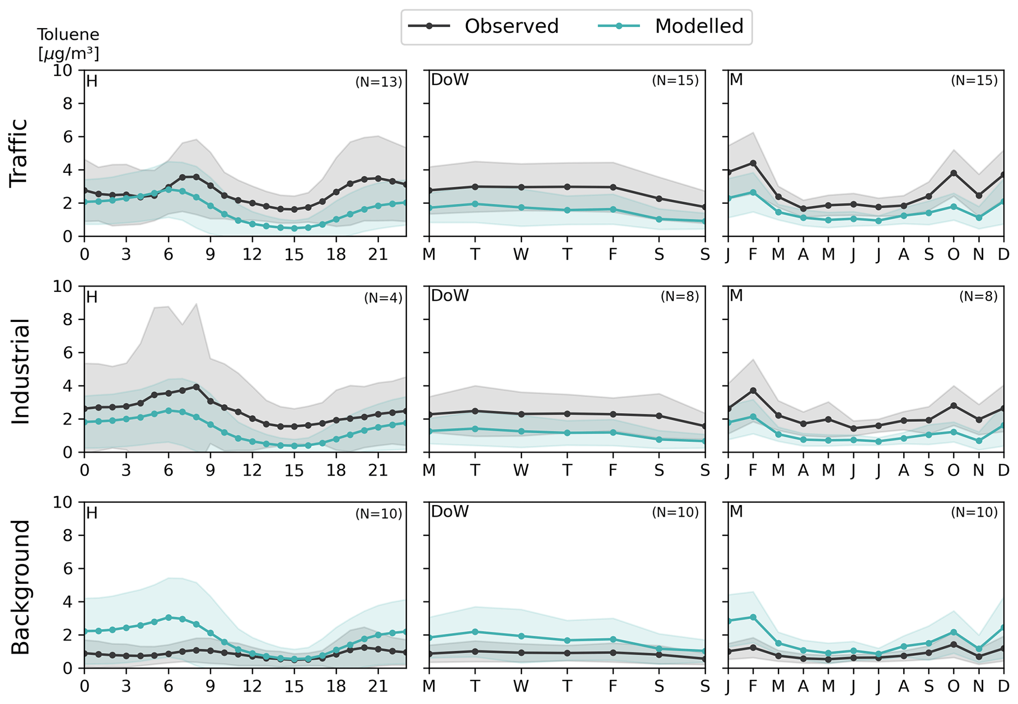
Figure 7Observed (black line) and modelled (blue line) toluene hourly (H), weekly (day of the week, DoW), and monthly (M) cycles (µg m−3) per station classification. The shaded region corresponds to the standard deviation variability.
3.2.2 Toluene
The highest toluene concentrations in 2019 were measured at two urban traffic stations located in Valencia (ES1239A, 5.95 µg m−3) and Valladolid (ES1631A, 3.77 µg m−3), respectively, followed by a suburban industrial station in Murcia (ES1627A, 3.63 µg m−3). It is worth mentioning that although toluene is one of the recommended VOCs for measurement in the AQD, no legal or recommended limits are defined by the EC or the WHO. The modelled results (see Fig. 5b) show that the maximum annual mean value is 6.85 µg m−3 and is located in Barcelona, where no measurements are available. Overall, the spatial pattern between observed and modelled annual mean values shows a good agreement, with urban areas being depicted as the main hotspots according to both sources of information.
In contrast to benzene, for which results were fairly consistent across sites (negative or close to 0 MB), heterogeneous results are observed for toluene (a mix of positive and negative MB). This information is also supported by Fig. E1b in Appendix E. A significant overestimation of the modelled concentrations is observed in Madrid's urban and suburban areas (between 0.71 and 2.81 µg m−3), except for one traffic station, which the model slightly underestimates (ES1564A, MB = −0.58 µg m−3). A similar, albeit to a lesser extent, overestimation is shown in central northern urban regions, specifically Cantabria (ES1580A, MB = 0.81 µg m−3 and NMB = 68.1 %) and Navarre (ES1602A, MB = 0.73 µg m−3 and NMB = 180 %). Most of the underestimations observed in urban stations occur at traffic monitoring stations. The biggest underestimation is found at one of these stations in Valencia (ES1239A, MB = −3.69 µg m−3). In suburban stations, the model tends to underestimate, with the exception of the station in Madrid (ES1193A, MB = 2.29 µg m−3). In other areas, modelled values are more aligned with observations, with MB being much lower. As previously shown, modelled toluene concentrations in the urban area of Barcelona are even higher than the ones modelled in Madrid. However, due to the lack of measurements in this region, we cannot conclude if these modelled levels are also overestimated, as in the case of Madrid.
The observed overestimations in urban stations suggest a potential limitation in the spatial disaggregation of specific dominant emission sources in these areas. This includes specific activities within the solvent sector, mainly from wood paint application and, to a lesser extent, industrial paint application and paint manufacturing. These sectors are of particular interest as they are the main toluene-emitting sources (see Sect. 3.1). The proxies considered in HERMESv3 for the spatial disaggregation of these three sectors include land use information related to industrial and commercial areas, population density information, and a shapefile containing the geographical location of individual paint manufacturing facilities, respectively. For instance, in activities related to the application of wood paint, we use the population as a proxy. This, combined with a coarse model resolution, causes modelled overestimations when compared to observations. However, validating or refining this information is challenging due to the scarcity of detailed and available data concerning these specific activities. Additionally, it is worth noting that this overestimation is not observed for benzene concentrations, as the speciation used for these sectors establishes zero benzene emissions.
Figure 7 shows the comparison between modelled and observed toluene hourly, daily, and monthly cycles per station classification, including the variability of the standard deviation as the shaded region. Modelled cycles are very consistent across stations. At the hourly scale, the model consistently reaches its morning peak between 1–2 h before the observations. While the shift between modelled and observed morning peaks is also reported for benzene concentrations (see Fig. 6), the model performs well for NO2 (see Appendix F). Further research is needed to understand the cause or combination of causes that could explain this shift. At traffic stations, the model effectively replicates hourly, monthly, and weekly cycles, although it tends to overestimate concentrations during the nighttime period. It is important to note that the results obtained at traffic stations compensate for the overestimation observed in the Madrid urban region, with underestimations reported in other urban traffic stations (see Fig. E1b). For industrial stations, the model accurately reproduces all observed cycles. However, it notably underestimates concentrations during weekends, suggesting a larger drop in concentrations during Saturday and Sunday than the one observed. This behaviour could be linked to an inadequate weekly distribution of emissions in certain facilities surrounding the industrial stations located in Tarragona, for which we assume that they close or significantly reduce their activity during weekends, while in reality they operate continuously. At background stations, a consistent overestimation of the model is observed, potentially attributed to an inaccurate spatial proxy applied to wood paint application. Currently, these emissions are disaggregated using population data, although they should be associated with industrial areas.
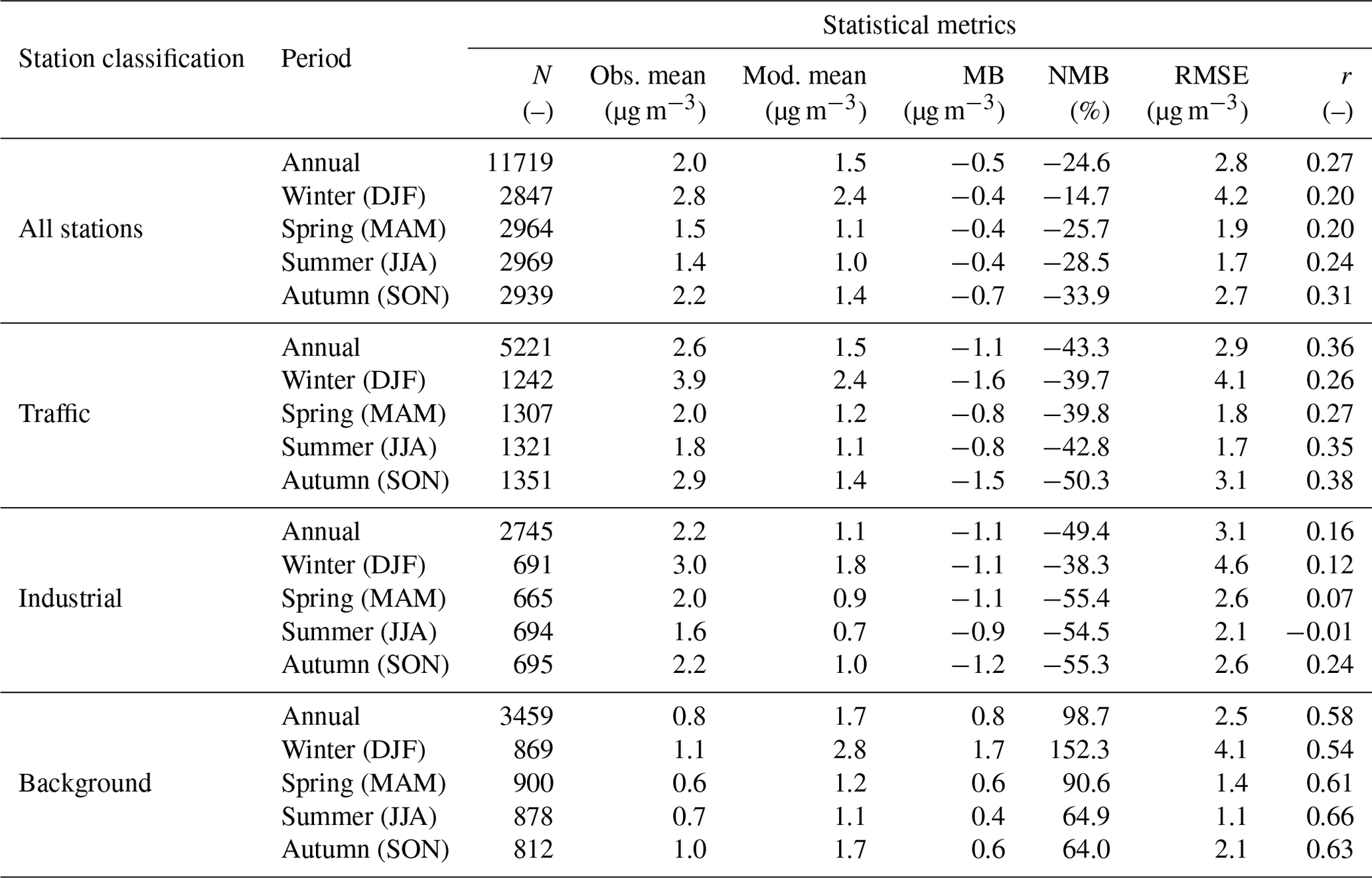
Table 3 provides statistical metrics for toluene, including N, observed mean, modelled mean, MB, NMB, RMSE, and r, for all stations and by station classification, both for the entire year and for each season. When considering all stations, the annual MB (−0.5 µg m−3) and NMB (−24.6 %) indicate a slight underestimation. Nevertheless, and as mentioned before, this is a result of compensation between the underestimations observed in traffic (MB = −1.1 µg m−3) and industrial (MB = −1.1 µg m−3) stations and the overestimations reported in background sites (MB = 0.8 µg m−3). The model consistently underestimates traffic and industrial stations in all seasons while overestimating background stations. The industrial stations generally have the highest RMSE values across all time periods, especially during winter (4.6 µg m−3). Furthermore, industrial stations consistently demonstrate the lowest r (below 0.16), which is close to zero during spring and summer. Background stations have the highest correlation but show a significant positive bias in annual and seasonal means, where for winter the highest NMB values are reached (greater than 100 %). This could be related to the increase in residential wood combustion emissions during this period. Additionally, as previously mentioned, the overestimations in background stations are mainly related to overestimations of the emissions from the solvent sector, mainly from paint application.
Table 3Seasonal and annual statistics for N, observed mean, modelled mean, MB, NMB, RMSE, and r per station classification for toluene in Spain in 2019 obtained with MONARCH.
3.2.3 Xylene
In Spain, the highest xylene concentrations in 2019 were measured at two industrial stations, in Palencia (ES1298A, 6.18 µg m−3) and Valladolid (ES1356A, 5.98 µg m−3), followed by a traffic station also located in Valladolid (ES1631A, 3.72 µg m−3). The two industrial air quality stations are located near (<1 km) two car manufacturing facilities.
Modelled maximum concentrations (2.53 µg m−3) are reported in Galicia on the northeast coast of Spain (see Fig. 5c). The levels are mainly driven by the presence of a car manufacturing facility. However, similar concentrations are also modelled in the urban areas of Barcelona (2.51 µg m−3) and Madrid (2.50 µg m−3). Out of these three regions, measured values are only available in Madrid, showing smaller concentrations (average of 1.16 µg m−3) compared to MONARCH. As in the case of toluene, and despite being recommended for VOC measurement in the AQD, no legal limits are established for xylene.
The pattern observed between modelled values and observations shows overall good performance of the model, with MB close to 0 (see Fig. E1c in Appendix E). Despite this, there are some exceptions with some traffic stations showing slight underestimations, an industrial station showing a slight overestimation in Madrid (ES1565A, MB = 0.88 µg m−3), and two stations that stand out as highly underestimated (ES1298A, MB = −5.91 µg m−3; ES1356A, MB = −5.02 µg m−3). These last stations are the ones that report the largest annual mean values and are located near car manufacturing industries, as described before. These underestimations were also identified for benzene, although they were more pronounced for xylene. The strong bias suggests that the emissions from this industrial activity are highly underestimated. This aspect is further analysed in Sect. 3.3.1.
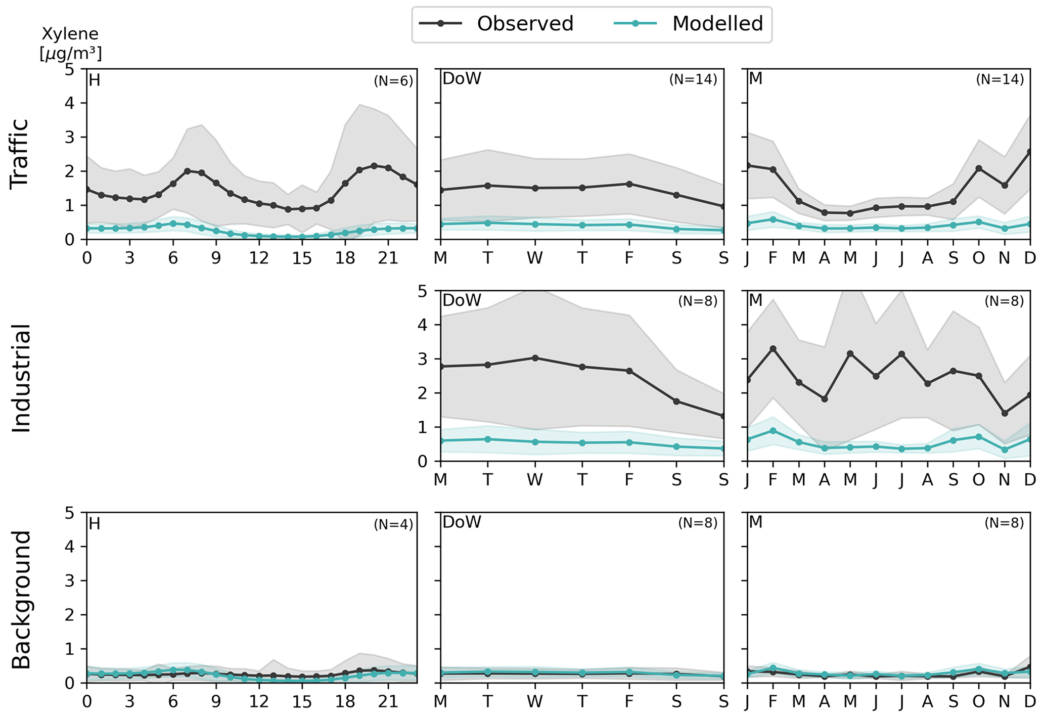
Figure 8Observed (black line) and modelled (blue line) xylene hourly (H), weekly (day of the week, DoW), and monthly (M) cycles (µg m−3) per station classification. The shaded region corresponds to the standard deviation variability.
Figure 8 shows the comparison between modelled and observed xylene hourly, daily, and monthly cycles per station classification, including the variability of the standard deviation as the shaded region. For traffic stations, the levels observed during spring and summer have a smaller bias than during the winter months. This suggests that traffic emissions related to cold-start emissions, as well as emissions from other non-road mobile sources (e.g. construction machinery, lawn, and garden equipment) influencing measured levels in these environments, might be underestimated. Despite the bias, the model effectively reproduces the weekly cycle, accurately capturing the weekend decrease. At the hourly scale, the already discussed shift between observed and modelled peaks for benzene and toluene also occurs for xylene, requiring further investigation.
The hourly cycle is not presented in the figure for industrial stations as only one station measuring xylene hourly is available. This limitation makes drawing conclusive insights for this type of station challenging. Overall, the model is highly underestimating for this station classification. Regarding the weekly cycle, the model presents a flatter profile compared to the observed one. This suggests that the facilities near the stations either operate primarily during the week or have lower production on weekends. When examining the monthly cycles, distinctive patterns are observed for measured and modelled values. In the first case, noticeable peaks occur during the summer months, which are not captured by the model. On the other hand, MONARCH successfully replicates the observed peaks in February, October, and December. As previously mentioned, the industrial stations near car manufacturing facilities show a significant negative bias. This indicates uncertainty in the emission estimates for these activities (see Sect. 3.3.1 for more details).
For background stations, we observe significantly lower values when compared to other station types. This is primarily attributable to the fact that most of these stations are located in small urban areas (e.g. Langreo in Asturias, and Mérida and Badajoz in Extremadura) and, therefore, are not so heavily influenced by main urban hotspots such as Madrid or Barcelona. Analysing the cycles, we note that the model performs reasonably well but tends to overestimate slightly.
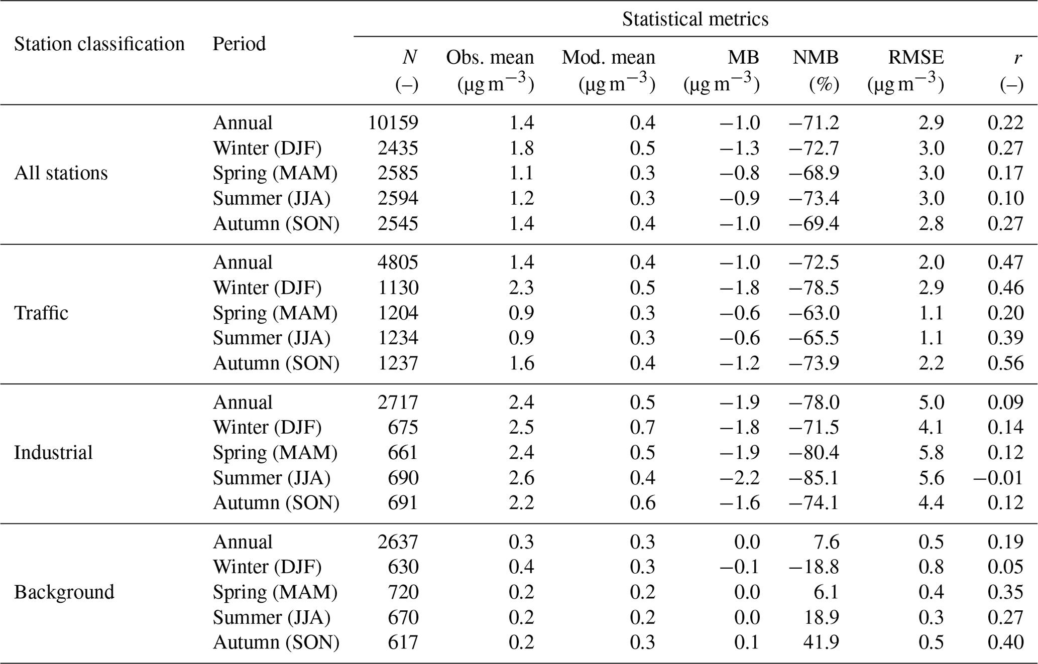
Table 4 provides statistical metrics for xylene, including N, observed mean, modelled mean, MB, NMB, RMSE, and r, for all stations and by station classification, both for the entire year and for each season. The annual statistics for all stations show an average xylene concentration of 1.4 µg m−3 with a model mean of 0.4 µg m−3, where the NMB is −71.2 %. The correlation coefficient (r) for the year is 0.22, suggesting a weak positive correlation while showing a moderate RMSE of 2.9 µg m−3. The correlation is lower during spring and summer (0.17 and 0.10, respectively) and bigger during autumn and winter (both 0.27). However, seasonal NMB values show the highest underestimation during summer (−73.4 %) and the lowest during spring (−68.9 %). The low correlation between observations and modelling results is mainly attributable to the low correlation registered at industrial stations.
Traffic stations exhibit a high seasonal variability, with winter having the highest observed mean concentration (2.3 µg m−3) and spring/summer (0.9 µg m−3) the lowest. Modelled means show 0.5 µg m−3 during winter and 0.3 µg m−3 for spring/summer. During winter, the model performs the poorest with the highest NMB at −78.5 % but maintains a moderate correlation (r) of 0.46. During spring, the model shows the lowest NMB (−63.0 %) but also in terms of correlation (0.20). The low correlation implies that the model during the spring season does not accurately capture the variations in xylene concentrations, which might be missing important non-linear patterns or variability more pronounced during spring. Despite this, traffic stations generally have the highest correlation values.
Among all the classifications, industrial areas exhibit the biggest annual observed (2.4 µg m−3) and modelled (0.5 µg m−3) values but also the most significant underestimation, with an NMB of −78.0 % and the highest RMSE of 5 µg m−3. Additionally, these areas consistently display the lowest correlation, which is generally weak across all seasons. The model consistently underestimates xylene concentrations in industrial areas throughout the year, with the highest NMB occurring during summer (−85.1 %) and the lowest during winter (−71.5 %). The weak model performance in these areas arises from the coarse resolution and uncertainties in modelling meteorology, as well as underestimation of emission sources and unaccounted for specific industrial operations like maintenance activities or leaks.
For background stations, unlike the other station classifications, the model tends to slightly overestimate with a NMB of 7.6 %. In terms of seasonality, the largest overestimations occur during autumn (MB = 0.1 µg m−3 and NMB = 41.9 %). The correlation between observed and modelled values generally leans towards a positive value but remains weak, ranging from 0.27 to 0.40, except for winter, where the correlation drops to approximately 0. This particular anomaly in winter can be primarily attributed to big peaks observed in a specific station in Asturias (ES1353A).
Table 4Seasonal and annual statistics for N, observed mean, modelled mean, MB, NMB, RMSE, and r per station classification for xylene in Spain in 2019 obtained with MONARCH.
3.3 Sensitivity analysis
Based on the discussion and findings presented in Sect. 3.2, we have conducted a series of sensitivity runs to explore and identify less-represented or poorly understood processes and emissions from specific sectors. The selected sectors, including the manufacturing industry (i.e. refineries, coke ovens, and car manufacturing facilities) and road transport (i.e. mopeds and motorcycles), were previously identified as potentially driving some of the main discrepancies between observed and modelled results. This identification was based on their proximity to air quality stations that were consistently underestimating, leading to the hypothesis that these sectors are likely the primary contributors to the observed bias. To assess this, we either estimated alternative emissions (using available information on EFs and activity data) or used different available datasets. The following subsections describe for each sector the approaches considered to derive alternative emission estimates and their impact on the modelling results.
3.3.1 Industrial emissions: refineries, coke ovens, and car manufacturing industries
The sensitivity analysis for the industrial sector focuses on emissions from three types of facilities: refineries, coke ovens, and car manufacturing industries. As previously discussed in Sect. 3.2.1 and 3.2.3, the benzene and xylene industrial stations where the model exhibits the largest bias are all located near these types of facilities. Figure I1 in Appendix I displays the locations of the facilities and air quality stations nearby that are considered for the sensitivity analysis.
The HERMESv3 plant-level industrial emissions considered in the results discussed in Sect. 3.2 are derived from the LPS database for refineries, car manufacturing industries, and one coke oven facility, as well as from PRTR-Spain for the remaining coke oven facilities. It is important to note that the non-methane volatile organic compound (NMVOC) emissions reported by PRTR are generally calculated or estimated, while for NO2 the values are measured and, in fewer cases, are calculated. It is essential to acknowledge that estimating or calculating emissions without direct comparisons to measured emission fluxes can introduce significant uncertainties and should be approached with caution. For example, in PRTR, for refineries, NO2 values are mainly obtained through direct measurements, with differences from the LPS database across different facilities averaging below 36 %. However, for VOCs, the differences are substantial, with the smallest difference for a specific facility being 50 %. Appendix F shows hourly, weekly, and monthly cycles of NO2 per station classification for the stations measuring VOCs. As shown in Fig. F1, the model generally performs better for NO2 than for VOCs. While a direct comparison may be challenging due to potential differences in sources and processes, this still highlights the considerable uncertainty in VOC emission estimates. For the sensitivity test, alternative emissions were proposed for each facility type, and they are discussed in detail later.
Figure 9 shows a comparison of the annual NMVOC emissions (i.e. BTX and other NMVOC) derived from the LPS database and PRTR-Spain for each Spanish refinery. Note that both the LPS database and PRTR-Spain only report total NMVOC emissions and that the split of these onto BTX and other VOCs was done considering the profiles reported by Oliveira et al. (2023). The comparison between the two datasets reveals dramatic discrepancies. LPS total emissions (1.6 kt) in this type of facility are more than 7 times lower than the estimated derived from PRTR-Spain (11.8 kt). Except for two facilities, PRTR-Spain consistently reports much larger emissions than the LPS database, with differences being up to a factor of 38. The source of these discrepancies are currently unknown as both datasets should follow a similar methodology. In all the facilities, benzene is the largest emitted species out of the BTX group (80 %). This is consistent with the fact that the speciation profiles used for the activities emitting NMVOCs in refineries (e.g. petroleum products processing or storage and handling of products) consistently account for a bigger fraction of benzene compared to toluene and xylene (Oliveira et al., 2023). For the sensitivity test, we replaced the original LPS emissions with the values reported by PRTR-Spain.
For car manufacturing facilities, total NMVOC emissions reported by the LPS database (1.27 kt) and PRTR-Spain (1.39 kt) are very similar. The emissions calculated in the LPS database for these facilities used a tier 3 approach from the EMEP/EEA guidelines (EEA, 2019). This approach is based on surveys of individual facilities and considers the amount of VOCs produced minus the amount of VOCs eliminated, resulting in the total VOCs emitted per facility. Considering the large underestimation of xylene concentrations in the stations located near this type of facility (Sect. 3.2) and the fact that independent speciation profiles from the literature indicate a similar amount of xylene emitted from this activity (between 5 % and 10 %, Oliveira et al., 2023), we hypothesise that the low performance of the model is linked to an underestimation of the total NMVOC reported by the LPS database for these facilities. Therefore, we calculated alternative emissions by multiplying the EFs reported by EMEP/EEA guidelines by the annual number of cars produced at each facility in 2019 (País, 2020). New emission estimates (3.8 kt) are around 240 % larger than the LPS estimates (1.1 kt) (see Fig. 9). The considerable differences observed when applying the different approaches, i.e. tier 1 and tier 3, show the significant uncertainty associated with VOC emission estimation. The differences could be due to a missing fraction of the products used in the mass balance or uncertainties in the emission processes and emission factors. For the paint application activity, the speciation profiles used reports zero benzene, so as a result, no impacts are expected on benzene observations. Consequently, this sensitivity analysis for these facilities does not address the underestimations observed for benzene. It is hypothesised that emissions from car manufacturing facilities are underestimated, although we were unable to estimate emissions for other activities.
For coke ovens, no alternative emission estimate exists besides the ones provided by PRTR-Spain. For two of the three facilities, the emissions reported by PRTR were measured and therefore should not be underestimated. The fugitive emissions from several activities in coke oven plants were identified to be a significant source of pollution (Aries et al., 2007). So, we hypothesise that the large benzene bias observed in the two industrial stations located near coke oven facilities (see Sect. 3.2) is linked to the non-inclusion of fugitive emissions in the PRTR-Spain (i.e. from charging, door and lid leaks, off-take leaks). This hypothesis is consistent with the fact that most of these NMVOC fugitive emissions are composed of benzene, with an average contribution of 57 % (Aries et al., 2007). To fill in this gap, we performed a bottom-up estimation of these emissions using information on the total Spanish coke production for 2019 (MITECO, 2019), the production capacity of each facility to distribute the total production, and EFs sourced from Aries et al. (2007) and references therein, covering five distinct activities linked to fugitive emissions: fugitive door (7.1 g t−1 of coke), charging hole lid (4.4 g t−1 of coke), soaking (7.1 g t−1 of coke), and coal charging (7.7 g t−1 of coke). This increased total NMVOC and benzene emissions in coke ovens by 32 t (+25 %) and 21 t (+33 %), respectively (Fig. 9). Compared to the increases in emissions for the other sectors, the addition of the fugitive emissions in coke ovens is expected to have a limited impact on the results.
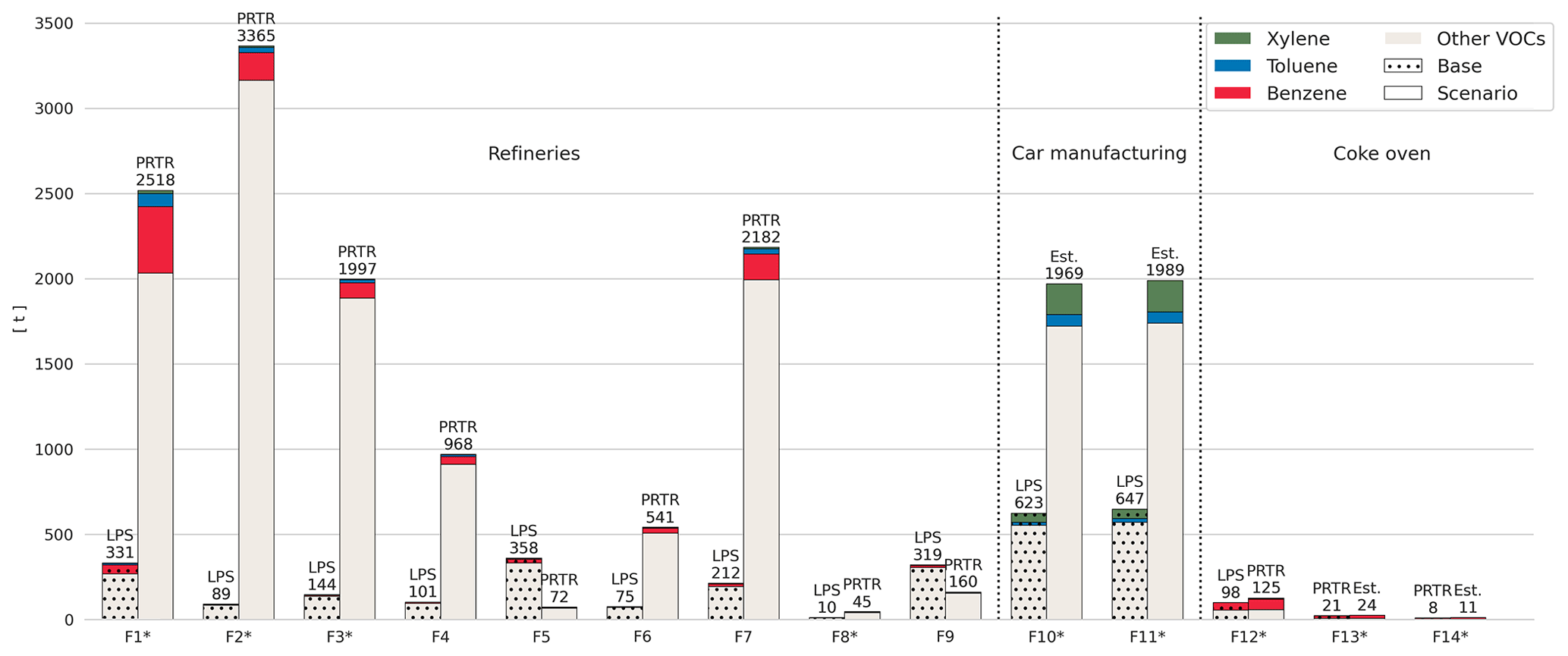
Figure 9Comparison between the baseline and the industrial scenario of total VOC emissions (t) in 2019 for 14 facilities in Spain. Each bar shows the total emissions and the source of the data (i.e. PRTR or LPS) or if it was estimated (Est.) for this work. The asterisk (*) indicates that the facility is located near an industrial air quality monitoring station.
Figure 10 shows the comparison between observed and modelled benzene, toluene, and xylene averaged monthly cycles at each selected industrial air quality stations, as well as the variability of the standard deviation as the shaded region (see Fig. I1). Modelled concentrations include the results obtained using the baseline and modified emissions. To ensure the robustness of our sensitivity analysis, observed values were filtered to exclude outliers by retaining data points within 3 standard deviations from the mean (i.e. z-score threshold of 3). In addition, Tables 5 and 6 summarise the comparison between annual statistics (MB, NMB, RMSE, and r) obtained in each station when using each emission dataset.
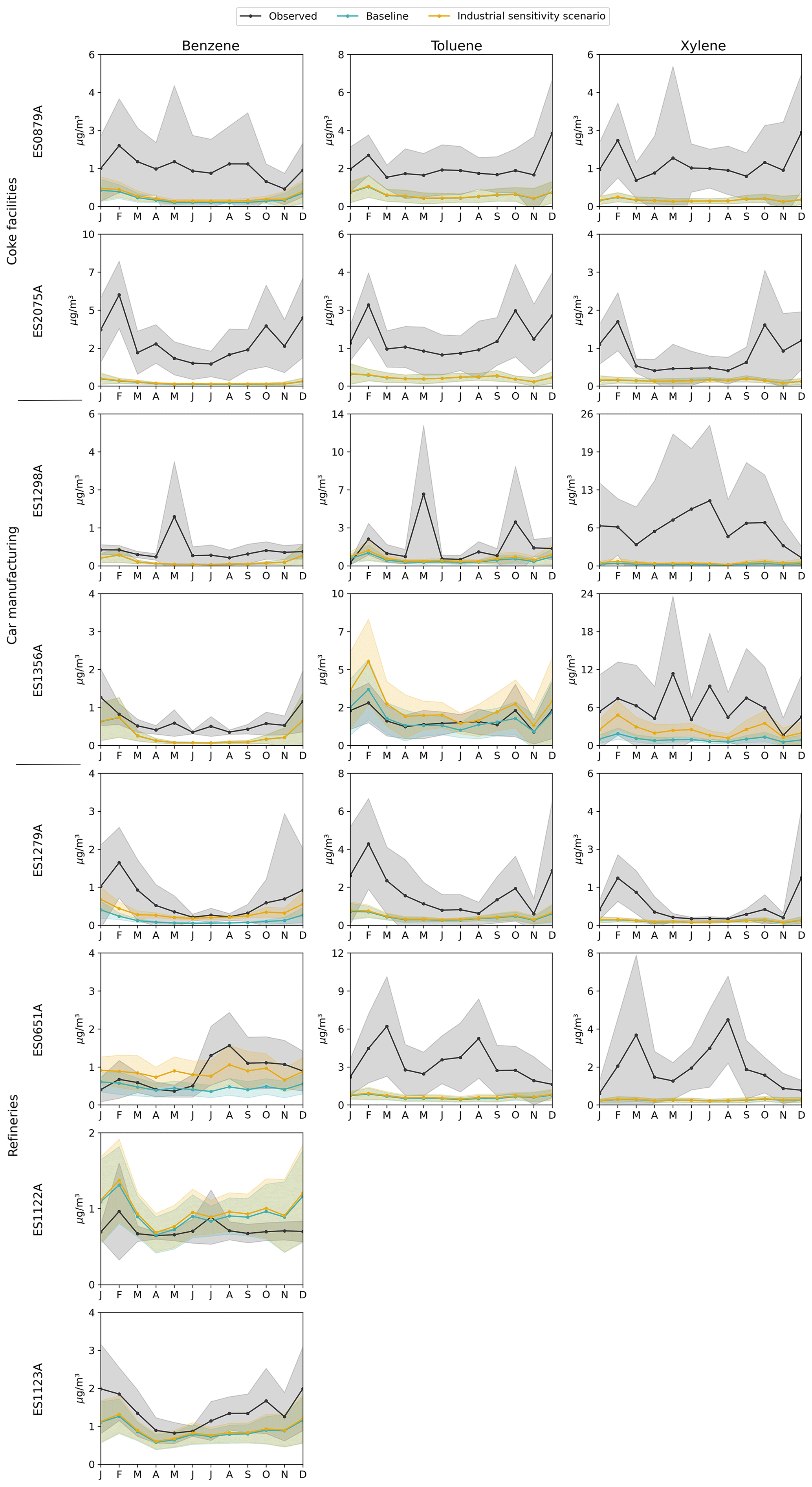
Figure 10Comparison of the monthly variability of benzene, toluene, and xylene concentrations from baseline (blue) and the industrial sensitivity scenario (orange) against observations (black) in 2019 for each industrial monitoring station. The shaded region corresponds to the standard deviation variability.
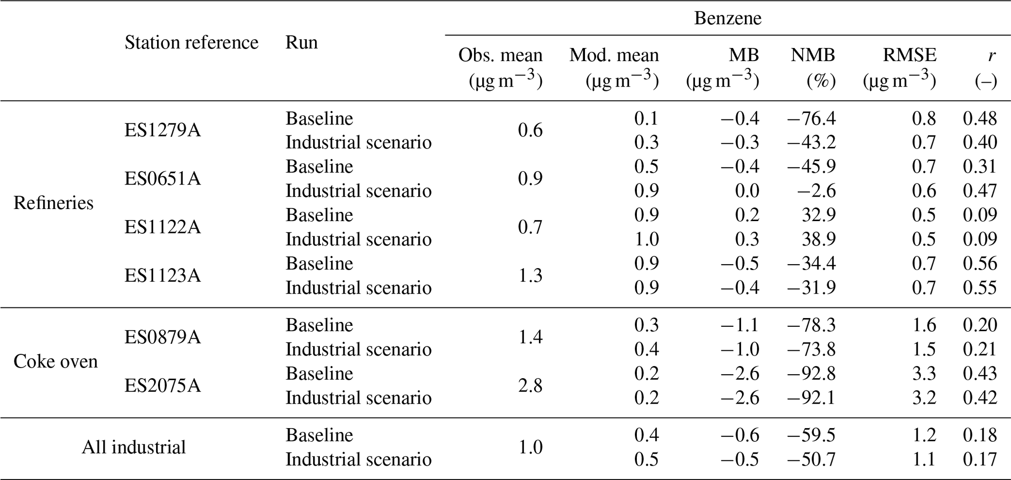
For benzene, the impact of modifying the industrial emissions on the model performance is heterogeneous across stations. Considerable improvements are observed in stations next to refineries, while the ones located near coke ovens continue presenting similar underestimations. Overall, industrial benzene concentrations remain significantly underestimated, with the NMB being shifted from −59.5 % to −50.7 %, reflecting a modest improvement primarily attributed to the limited increases in emissions from coke ovens (see Fig. 9). The low improvements observed in stations near coke ovens (distance below 700 m) and the fact that these stations report the highest annual mean concentrations indicate that the refined emissions are still missing relevant processes emitting benzene in these types of facilities. The improvements are considerably more pronounced for stations close to refineries when compared to those near coke ovens. For instance, at station ES1279A, the NMB decreased from −76.4 % to −43.2 %, and the RMSE improved from 0.8 to 0.7 µg m−3. As previously mentioned, the changes in emissions affect total NMVOCs, so the impacts observed for each VOC species vary due to the speciation profile used. For example, for station ES0615 (see Fig. 10), the model's performance significantly improved for benzene, reducing the NMB from −45.9 % to −2.6 % and increasing the correlation from 0.31 to 0.47. In contrast, the impacts on toluene and xylene are minimal. This could indicate a limitation arising from the speciation profiles used, although the fractions were similar compared to other available profiles. The impact is less pronounced for the other stations near refineries, likely due to their positioning relative to the emission sources (distance between 2 and 3 km). In addition, the limited impact observed in certain locations may not solely be due to emission uncertainties. The results might be influenced by meteorology biases in parameters, such as PBL or wind fields. These factors together with the grid resolution of the model may explain the uncertainties identified in the results, especially when considering emissions from industrial point sources.
Table 5Comparison of annual statistical metrics (N, observed mean, modelled mean, MB, NMB, RMSE, and r) for benzene in Spain in 2019 obtained with MONARCH for the baseline and the industrial sensitivity analysis.
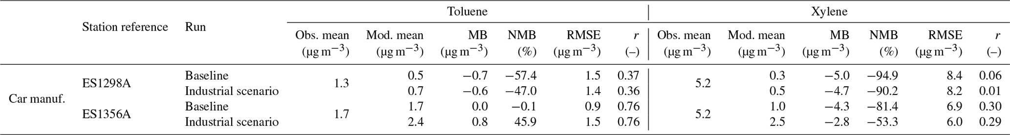
For toluene, Table 6 compares statistical metrics for the baseline and the industrial sensitivity analysis for the two stations near car manufacturing and the overall impact on industrial stations. For the station ES1298A, the MB and NMB slightly decreased from −0.7 to −0.6 µg m−3 and −57.4 % to −47.0 %, respectively. At station ES1356A, the model was performing well with an NMB of −0.1 %, and now it increased to 45.9 %, while the correlation is constant as 0.76. While the model was performing well for this location, it was partially explained by a compensation between industrial emission underestimations and overestimations from the solvent sector, previously identified in Sect. 3.2.2. So, increasing the emissions from this facility results in a degradation of the models' performance (see Fig. 10).
For xylene, the adjustment of industrial emissions improved the model's capability to reproduce the observed monthly cycle for stations near car manufacturing facilities (see Fig. 10). Table 6 summarises the changes in the MONARCH's performance at the two stations close to the car manufacturing industries, as these are the facilities where xylene emissions have increased the most when adjusting the industrial VOC emissions (see Fig. 9). Improvements in MB, NMB, and RMSE can be observed in both locations, but most notably in ES1356A, with the MB and NMB decreasing from −4.3 to −2.8 µg m−3 and from −81.4 % to −53.3 %, respectively. For station ES1298A, there are slight improvements; the NMB decreases from −94.9 % to −90.2 %, and the RMSE decreases from 8.4 to 8.2 µg m−3, although the model is still highly underestimated. Despite the overall improvements, it is evident that the model still underestimates xylene concentrations, suggesting potential uncertainties in reproducing meteorological characteristics, missing sources or emission underestimations. It is worth noting that in both stations, the model still struggles to reproduce the changes in observed concentrations as the correlation stays very low. This is mainly due to frequently observed episodes, evidenced by the highest standard deviation variability. Daily means exceed 15 µg m−3 in both stations, even after removing outliers. These occurrences may be linked to specific activities within the nearby facilities, which are not accounted for in our model.
Table 6Comparison of annual statistical metrics (observed mean, modelled mean, MB, NMB, RMSE, and r) for toluene and xylene in Spain in 2019 obtained with MONARCH for the baseline and the industrial sensitivity analysis.
3.3.2 Road traffic sector: mopeds and motorcycles
The sensitivity analysis concerning the traffic sector, particularly emissions from mopeds and motorcycles, arises from the underestimations identified in Sect. 3.2. We identified that urban traffic stations in large cities, such as Barcelona and Valencia, exhibited significant underestimations for benzene, while in other major urban areas, such as Madrid, the modelled and observed results are pretty in line. This discrepancy suggests a potential misrepresentation of local traffic sources characteristic of these cities, specifically due to the significant contribution of mopeds and motorcycles to the road transport sector, which is further described next.
Figure 11 shows the monthly comparison of NO2 and benzene concentrations for urban traffic stations in Madrid, Barcelona, and Valencia. For the traffic stations located in Madrid, the model was able to reasonably reproduce both NO2 (NMB = −23.96 %) and benzene (NMB = −9.64 %) levels. In the case of Barcelona and Valencia, we observed that while NO2 levels (NMB = −24.77 % and NMB = −14.77 %, respectively) are also reasonably well reproduced, benzene concentrations are significantly underestimated (NMB = −69.97 % and NMB = −76.53 %, respectively). Measured benzene levels in Barcelona are much higher (2.81 µg m−3) than the ones reported for Madrid (0.51 µg m−3). This is a characteristic that MONARCH fails to reproduce, as the modelled concentrations are similar in all urban traffic sites. Observed benzene concentrations in Barcelona and Valencia achieve their maximum values during winter (up to 5 µg m−3), showing a marked seasonality that is not registered in any of the Madrid urban traffic stations and that the model is not capable of reproducing. Notably, looking at background levels in Barcelona, as seen in station ES1856A (see Fig. I2), the model can perform reasonably well for both NO2 (NMB = 13.26 %) and benzene (NMB = −18.20 %). For Valencia, there are no available background stations measuring benzene. Since the background levels are correctly reproduced in Barcelona, this leads to the conclusion that the main issue should be related to a local traffic source.
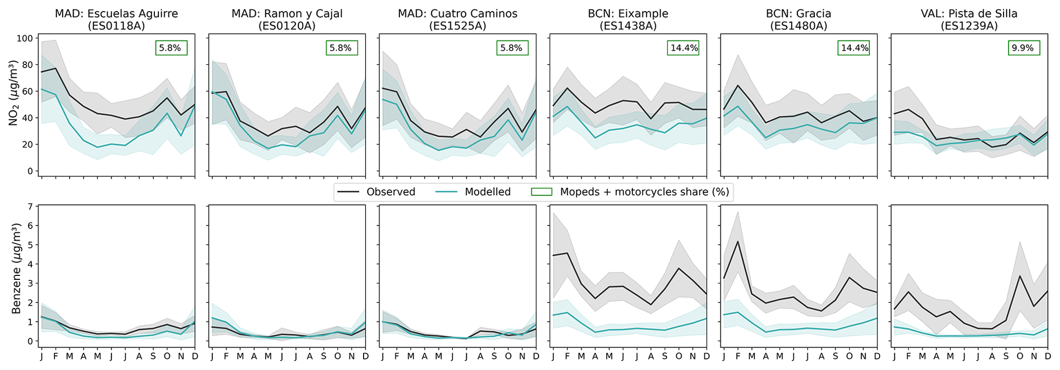
Figure 11Monthly comparison of NO2 and benzene concentrations (µg m−3) at urban traffic stations in Madrid (MAD), Barcelona (BCN), and Valencia (VAL). The share of mopeds and motorcycles per city used in HERMESv3 is included.
Focusing on Madrid and Barcelona, both exhibit significantly different fleet compositions, with Madrid having a moped and motorcycle share of 5.8 % and Barcelona having a share of 14.4 %. Moreover, according to HERMESv3 results in Barcelona, mopeds and motorcycles contribute around 63 % to road transport benzene emissions. These results are in line with the remote sensing results obtained by Dallmann et al. (2019) for Paris in 2015, where the contribution of motorised two-wheeled vehicles was 46 % of road transport non-methane hydrocarbon emissions. Moreover, a quick analysis of measured benzene in European urban traffic stations showed that similar high annual mean values are found in other Mediterranean coastal cities, such as Genoa, Italy (2.70 µg m−3), and Athens, Greece (2.81 µg m−3). Notably, these countries are also known for having a significant share of mopeds and motorcycles (Yannis et al., 2007; Scorrano and Danielis, 2021). This reinforces the hypothesis of a possible benzene emission underestimation from mopeds and motorcycles.
The EFs from mopeds and motorcycles reported by the COmputer Programme to calculate Emissions from Road Transport version 5 (COPERT 5), which are used in HERMESv3, seem to align with alternative estimates (Saxer et al., 2006; Adam et al., 2010). Therefore, we assume the issue is related to the degradation factor, which in HERMESv3 is considered for petrol- and diesel-powered vehicles but not mopeds and motorcycles.
Following the methodology presented by EEA (2016) for petrol cars and light commercial vehicles, we used Eq. (1) to estimate correction factors accounting for different vehicle ages. To accomplish this, we utilised the linear regression constants for hydrocarbon (HC) emission factors based on odometer mileage (km) as provided by Tsai et al. (2018). We calculated the mean mileage for each moped/motorcycle category using the data provided by the ministry on kilometres travelled per category and year. The values used per vehicle category are in Appendix I in Table I1.
where Mcorr is the mileage correction factor for a given mileage (MMEAN), MMEAN is the mean fleet mileage of vehicles for which the correction is applied (km), AM is the degradation of the emission performance per kilometre, and BM is the emission level of a fleet of brand new vehicles. AM and BM are assumed to be constant and do not depend on the vehicle category.
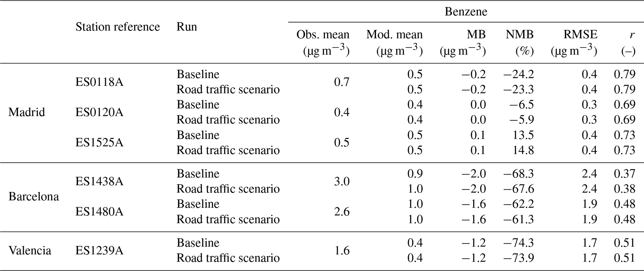
Implementing the mileage degradation for VOCs increased mopeds and motorcycle emissions by a factor of 2–3. Despite this, the impact on benzene concentrations is quite limited, with the model still significantly underestimating observed values in Barcelona and Valencia. Table 7 presents a comparison between the baseline and sensitivity analysis scenario, which incorporates the mileage degradation. The table summarises annual statistics (MB, NMB, RMSE, and r) obtained for traffic stations in Madrid, Barcelona, and Valencia. Overall, the NMB decreased (between −0.4 % and 1.0 %) for all the stations except for station ES1525A, located in Madrid, where the performance was slightly degraded (from NMB = 13.5 % to NMB = 14.8 %) with the scenario. Station ES1438A is the only station where the correlation increased, rising from 0.37 to 0.38.
We believe the model coarse spatial resolution (0.1° by 0.1°) may be playing a role in these results, as it is not capable of capturing the large influence of mopeds and motorcycles in the urban traffic areas of the city. Unlike vehicle passenger cars, whose spatial distribution across Barcelona's urban fabric is relatively homogeneous, mopeds and motorcycles in Barcelona mainly circulate in the inner city, where the two air quality urban traffic stations are located (Rodriguez-Rey et al., 2022). Performing simulations at a much finer spatial resolution (i.e. 1 km or less) would be needed to confirm this point. Despite this, it is evident that the emissions are still underestimated, suggesting that some sources are either not accurately represented in our model, are unaccounted for, or the uncertainties in atmospheric chemistry and meteorological effects are contributing factors. So, to improve the model's performance in these locations, it would be important to include city-specific characteristics that impact EFs (e.g. topography). For instance, Yang et al. (2021) estimated that uphill driving can significantly impact EFs, with an estimated factor of approximately 12 compared to baseline or downhill driving. Due to the different topography of Barcelona compared to Madrid, introducing this aspect into the model could lead to further improvements in its performance.
Additionally, despite the increases in emissions, the model's low performance could also suggest other issues, such as reproducing localised atmospheric and meteorological characteristics (e.g. PBL). Additionally, as seen in Appendix H, the measurement methods vary. In Barcelona, the stations use gas chromatography–mass spectrometry–flame ionisation detection (GC-MS-FID), while in Madrid, the stations use GC-MS. The differences in measurement methods could lead to several uncertainties and discrepancies in the observed values between both cities (e.g. interferences). Similarly, variations in measurement methods have also been identified as a factor influencing NO2 values (Steinbacher et al., 2007; Villena et al., 2012). While the experimental limitations of methodologies and instrumentation measuring VOCs are beyond the scope of this paper, they represent crucial variables to consider when performing model evaluations.
Table 7Comparison of annual statistical metrics (N, observed mean, modelled mean, MB, NMB, RMSE, and r) for benzene in Spain in 2019 obtained with MONARCH for the baseline and the road traffic scenario, which accounts for the mileage degradation.
4.1 Summary
VOCs significantly impact air quality and atmospheric chemistry and are key precursors for the formation of in O3 and SOA. Aromatic VOCs, such as benzene, toluene, and xylene (BTX), pose distinct health risks, which further justifies the importance of understanding their variability and mitigating their negative impacts. Nevertheless, comprehensive model-based evaluation studies on VOC species remain scarce in the literature.
The present work presents an assessment and evaluation of BTX primary emissions and concentrations in Spain by combining observations, emission inventories, and air quality modelling techniques. We run the HERMESv3 emission model to produce a gridded bottom-up inventory of VOC emissions and use it as input in the MONARCH chemical transport model to analyse the spatial and temporal variability of BTX surface concentrations across Spain. Estimated results are then compared to observed values reported by the Spanish official national air quality monitoring network. The intercomparison between modelled and observed levels allows identifying sources of uncertainty within the emission input, which we further explored through specific sensitivity test runs.
The following conclusions are obtained from the analysis of the bottom-up BTX emissions estimated with HERMESv3.
-
Total annual emissions in 2019 of benzene, toluene, and xylene over Spain reach 11, 26, and 12 kt, respectively. The spatial distribution of these emissions across Spanish regions varies across chemical compounds, but Andalusia, Catalonia, and the Valencian Community appear as major contributors for the three species.
-
Regarding dominating sources in urban areas, benzene is primarily emitted by the industrial sector (35 %–44 %), followed by traffic (29 %), while both xylene and toluene are primarily emitted by the industrial solvent sector (contributing around 89 % for toluene and 78 % for xylene), mainly from the industrial paint application. While domestic solvent use is one of the main emitting activities of total VOCs (11 %), its contribution to BTX emissions is relatively limited, constituting less than 1 % in the speciation profiles considered.
-
Regarding the spatial distribution, benzene emissions in urban areas are primarily attributed to the road transport sector (over 60 %), while outside of urban areas the residential sector dominates (> 90 %). For toluene and xylene, both urban and suburban areas are largely influenced by the industrial solvent sector (comprising 63 %–97 % of emissions), while in more rural areas the livestock and residential sectors play a more significant role.
The comparison between modelled and observed BTX concentrations and sensitivity test runs lead to the following conclusions.
-
Both observed and modelled Spanish benzene concentrations remain below the EU annual limit value.
-
Comparison results indicate a generally good spatial correlation between observations and model outputs. However, the highest modelled values were observed in areas lacking monitoring stations.
-
The model shows a good performance in replicating benzene concentrations within non-industrial areas, albeit with a tendency to underestimate, especially during winter. In contrast, the performance diminishes noticeably in industrial zones due to uncertainties linked to specific industrial activities, such as refineries, car manufacturing facilities, and coke ovens.
-
A sensitivity analysis was tested for the identified industrial activities by estimating alternative emissions considering different sources (i.e. from the PRTR and LPS databases or estimated for this work). The industrial sensitivity analysis overall showed some improvements, although the model is still strongly underestimating near some industrial sites. This underestimation may be linked to underestimations in the total emissions. Additionally, in some cases, the EFs may be more generic, lacking industry-specific nuances and thereby introducing uncertainty in the estimation of the emissions.
-
The model's more pronounced underestimations identified during winter can be attributed to several uncertainties and modelling limitations. For instance, in urban and suburban areas, underestimations are primarily influenced by residential wood combustion, which is less relevant in large cities. Additionally, it is important to note that the emission model only accounts for cold-start emissions in Madrid and Barcelona. Therefore, the model's performance in traffic stations during winter could be enhanced by incorporating cold-start emissions in all urban areas.
-
Observed benzene levels in Barcelona’s urban traffic areas were 5 times larger than the ones observed in Madrid. While the model performs well in replicating background station values in Barcelona, suggesting a potential underestimation of emissions from mopeds and motorcycles, caution is warranted when comparing model outputs against measurements obtained using different techniques (e.g. GC-MS in Madrid and GC-MS-FID in Barcelona) due to uncertainties and limitations for the different measurement methodologies.
-
Another sensitivity analysis was performed by incorporating mileage degradation factors for mopeds and motorcycles. The impact of this sensitivity analysis was shown to be very limited, which in part could be related to the resolution as it fails to capture the changes in urban areas. Despite this, from the results we conclude that the emissions from mopeds and motorcycles are still underestimated, although due to a lack of available literature, including EFs, we could not conduct further investigations and more work is needed in this area.
-
MONARCH's performance in traffic sites could be improved by incorporating additional sources related to the road transport sector. Other authors have identified relevant factors, for example, accounting for varied road grade characteristics' impact on the EFs (Yang et al., 2021).
-
For toluene, the model shows a good level of accuracy in replicating the hourly, monthly, and weekly cycles across various station classifications. However, it tends to underestimate the levels in traffic stations while significantly overestimating them in background stations.
-
The toluene overestimations are particularly pronounced in the Madrid area and, to a lesser extent, in stations located in central northern regions, such as Cantabria and Navarre. The model's limited performance in these regions may be attributed to inadequate proxies to spatially disaggregate emissions from activities within the industrial solvent sector, namely for wood paint application, which uses the population as a spatial proxy.
-
For xylene, the model effectively reproduced the hourly, monthly, and weekly cycles across different station classifications. However, significant underestimations were observed, particularly for traffic stations during the winter months, where the model struggled to replicate peak concentrations.
-
The most significant xylene underestimations were identified in industrial facilities near car manufacturing facilities, and these were particularly pronounced during the spring and summer months, especially on weekdays.
-
The industrial sensitivity analysis showed important improvements in the model's performance for stations near car manufacturing. However, it is still underestimating, indicating incorrect characterisation of specific activities contributing to VOC emissions.
-
MONARCH performs better in reproducing NO2 than VOCs in the stations considered. This could potentially be related to several factors, such as the fact that NOx industrial emissions are more robust due to better measure-based EFs, the fact that chemical mechanisms are designed to reproduce O3 and NO2 while major challenges remain to describe VOCs, limited constraints in key processes like VOCs dry deposition, and scarce availability of VOCs measurements which account for several uncertainties.
4.2 Implications for future research
As previously highlighted, a significant challenge in assessing the performance of the models arises from the inherent uncertainties from emissions, such as EFs and activity data, chemical mechanisms, and limitations associated with observational data.
For this work, we considered a total of 47 stations measuring benzene, 34 stations measuring toluene, and 30 stations measuring xylene. The spatial distribution reveals a notable absence of monitoring stations in south and north-western Spain, as well as in Barcelona for toluene and xylene. Another prominent limitation comes from the absence of quality continuous measurements. For example, in the case of stations monitoring benzene, after applying a 75 % temporal coverage threshold and implementing the GHOST quality filters, approximately 55 % of the available stations were dropped mainly due to the low temporal coverage. Furthermore, continuous measurements primarily target aromatic compounds, while data for other VOCs are often measured from short-duration campaigns and confined to specific locations. These limitations are crucial to consider since a comprehensive evaluation of VOC emissions and concentrations requires consistently high-quality data, both in terms of spatial and temporal coverage. Moreover, it is essential to take into consideration the uncertainties and limitations between measurement technologies when evaluating a model against observations. In addition, the usage of satellite data to monitor VOCs is emerging; for example, Franco et al. (2022) obtained emission rates for ethylene from satellite data, which were linked to big industrial facilities. This could be used in the future to better assess and evaluate the spatial distribution of modelled VOC levels and associated emissions.
The modelling simplifications to represent VOCs in chemical mechanisms are essential for computational efficiency. While necessary, they introduce uncertainties, with the main limitation for model evaluation being the restricted number of species with direct comparison to measurements. Future works using MONARCH should focus on including explicit species in the model, following a similar methodology to that implemented by Ge et al. (2024). This approach is key to extend the current work and ensure a direct comparison between modelled and observed species.
To conclude, this research enhances our understanding of VOC emissions and uncertainties while also contributing to the improvement of air quality models. By identifying limitations in emission sectors, chemical mechanisms, and observations, we pinpoint critical elements for enhancement. As demonstrated by Travis et al. (2024), improving VOC emissions and chemistry can aid in better describing urban ozone pollution, consequently supporting the design of more effective pollution control strategies. This is crucial as the upcoming study will evaluate the effects of specific VOC emission reduction strategies on air quality. Although the initial set of measures examined by Petetin et al. (2023) indicated limited impacts of anthropogenic VOC emission reductions on O3 Spanish levels, additional scenarios will be explored, focusing on assessing the impact on PM2.5. Given the significant health and environmental implications associated with fine particulate matter and the crucial role of VOCs in its formation through secondary aerosol formation, expanding our analysis will provide a better understanding of the effectiveness of these strategies in improving overall air quality.
This appendix provides the CB05 mechanism reactions and extensions implemented in MONARCH involving benzene (BENZENE), toluene (TOL), and xylene (XYL) and the respective species names in Table A1. Further information on the original CB05 mechanism and reactions is available in Yarwood et al. (2005).
Table A1Species names used for the CB05 mechanism reactions and extensions implemented in MONARCH regarding benzene, toluene, and xylene.
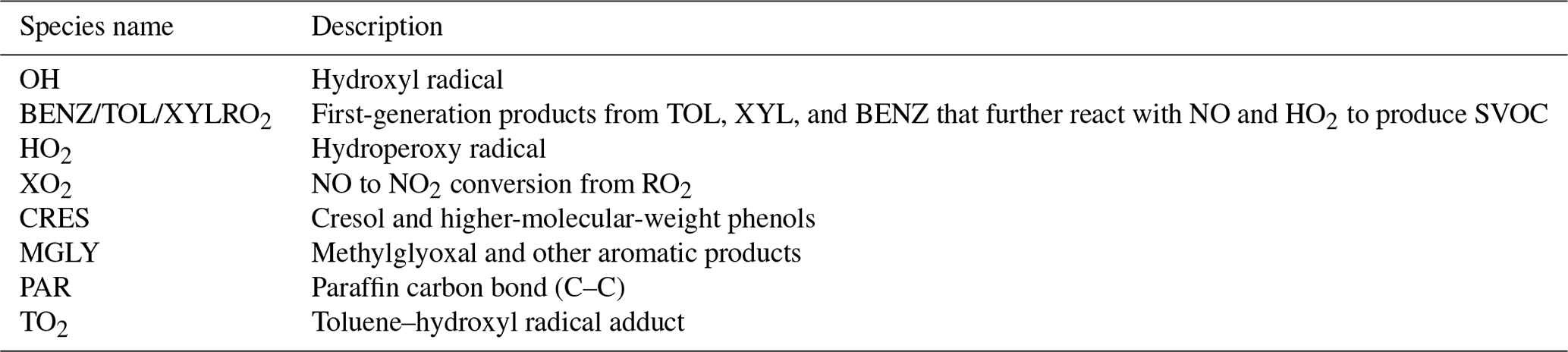
Table A2Reactions in the CB05 extended mechanism used in MONARCH for BTX.
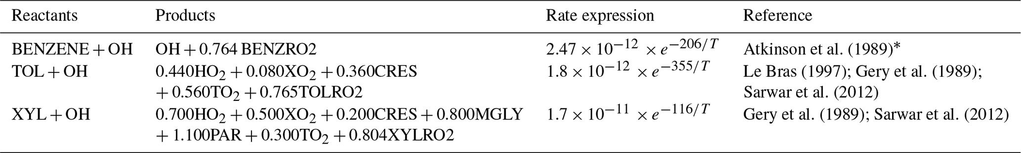
References are provided for the different reactions and rates. * Only the first-generation product that further reacts to produce SVOC is considered from the original reference.
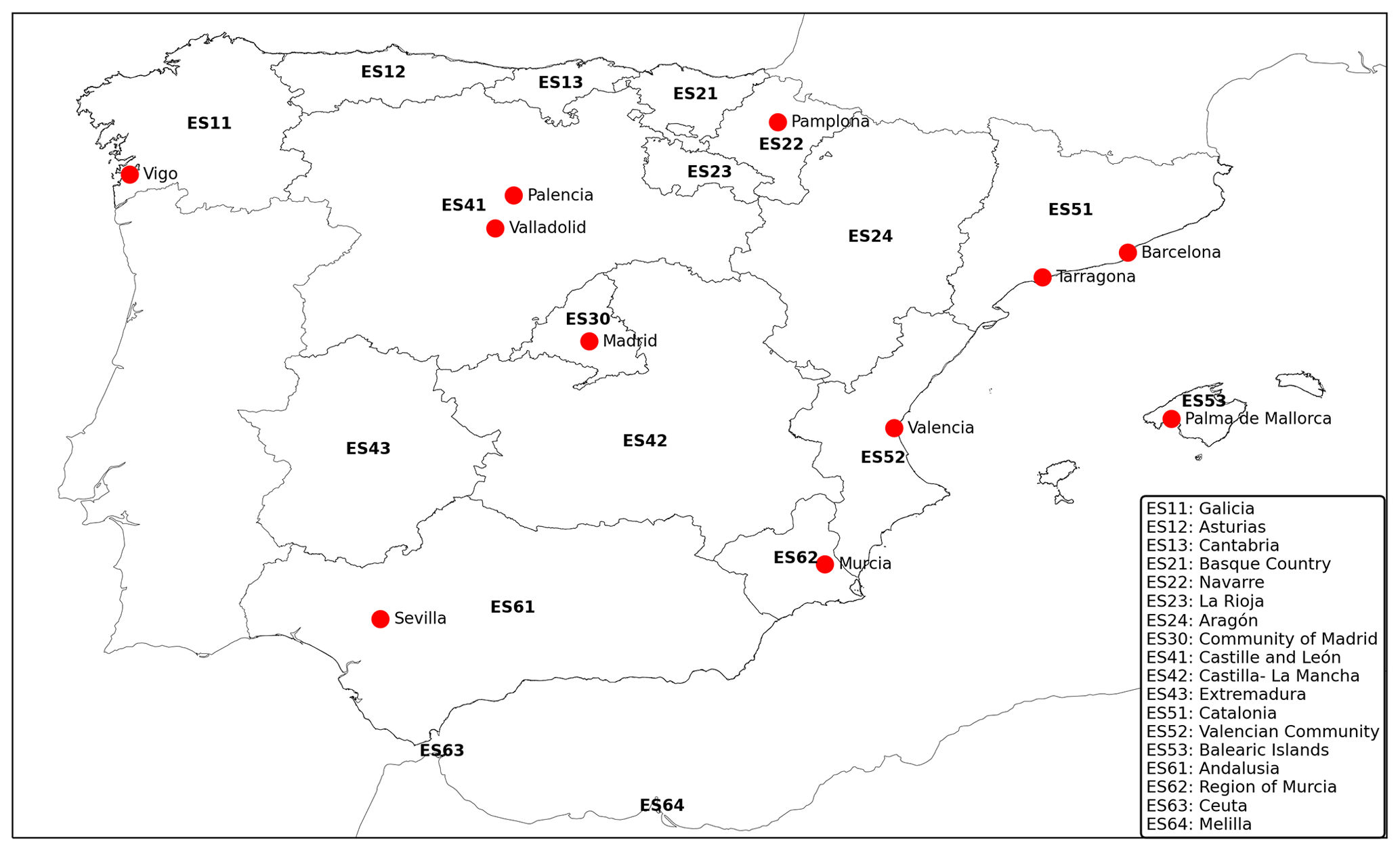
Figure B1Administrative Spanish NUTS2 regions and main cities mentioned in this work.
A quality assurance screening was applied to all observations using Globally Harmonised Observational Surface Treatment (GHOST) metadata, and all observations flagged were removed.
Table C1Description of the GHOST quality assurance flags used on the air quality observational dataset.
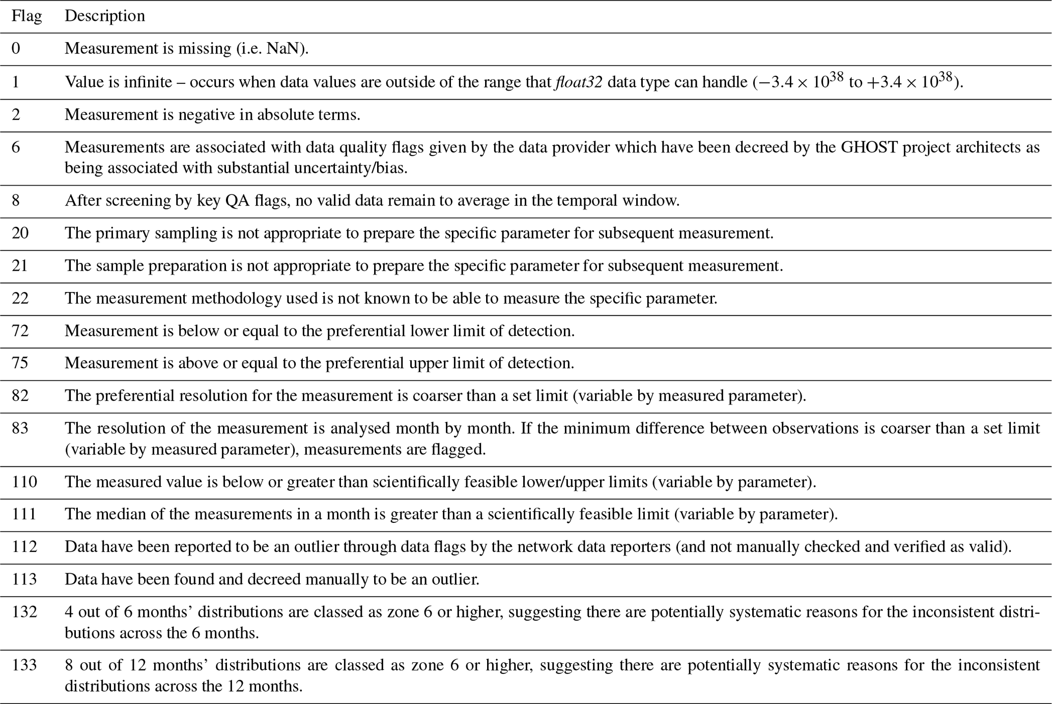
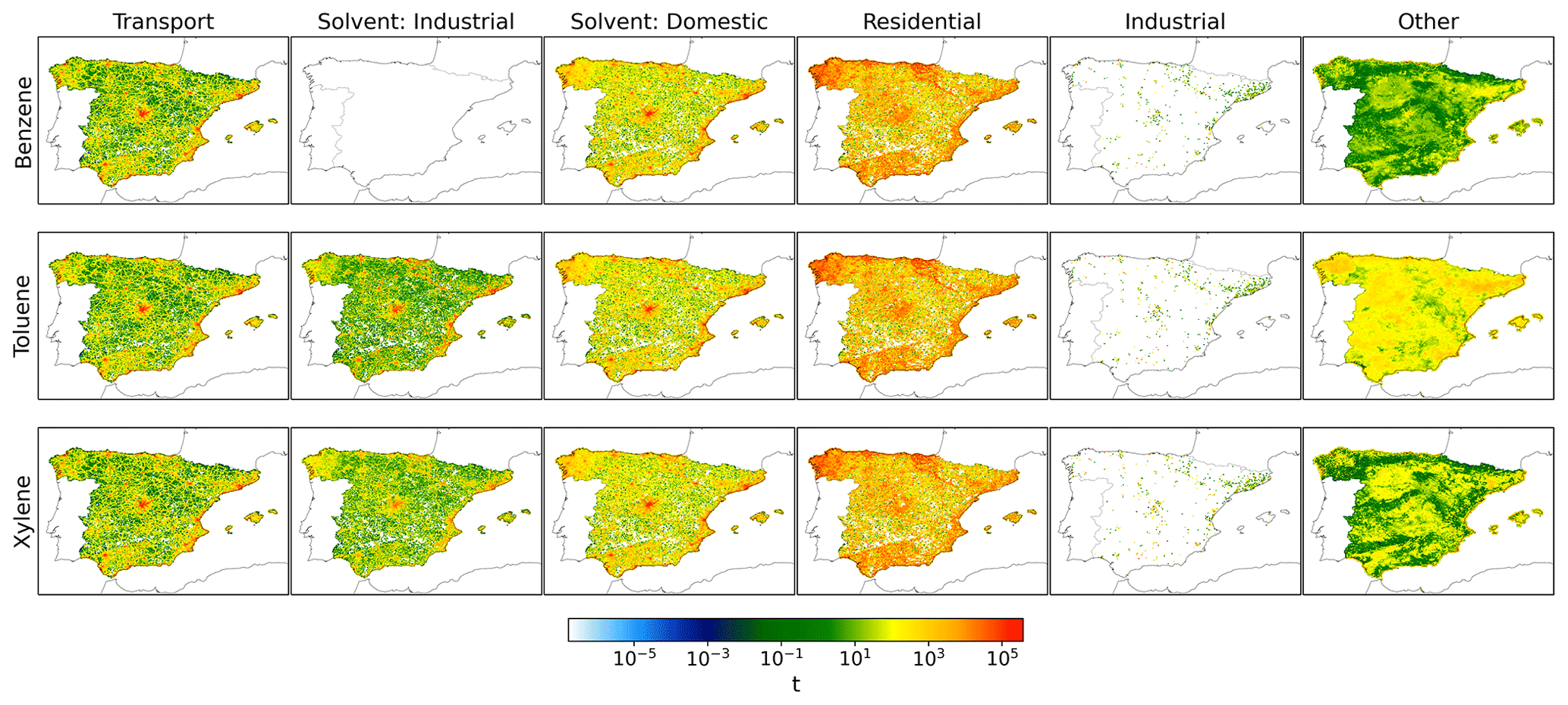
Figure D1Absolute contribution (t) of individual anthropogenic emission sources to total benzene, toluene, and xylene annual emissions in Spain in 2019 per grid cell (4 km by 4 km).
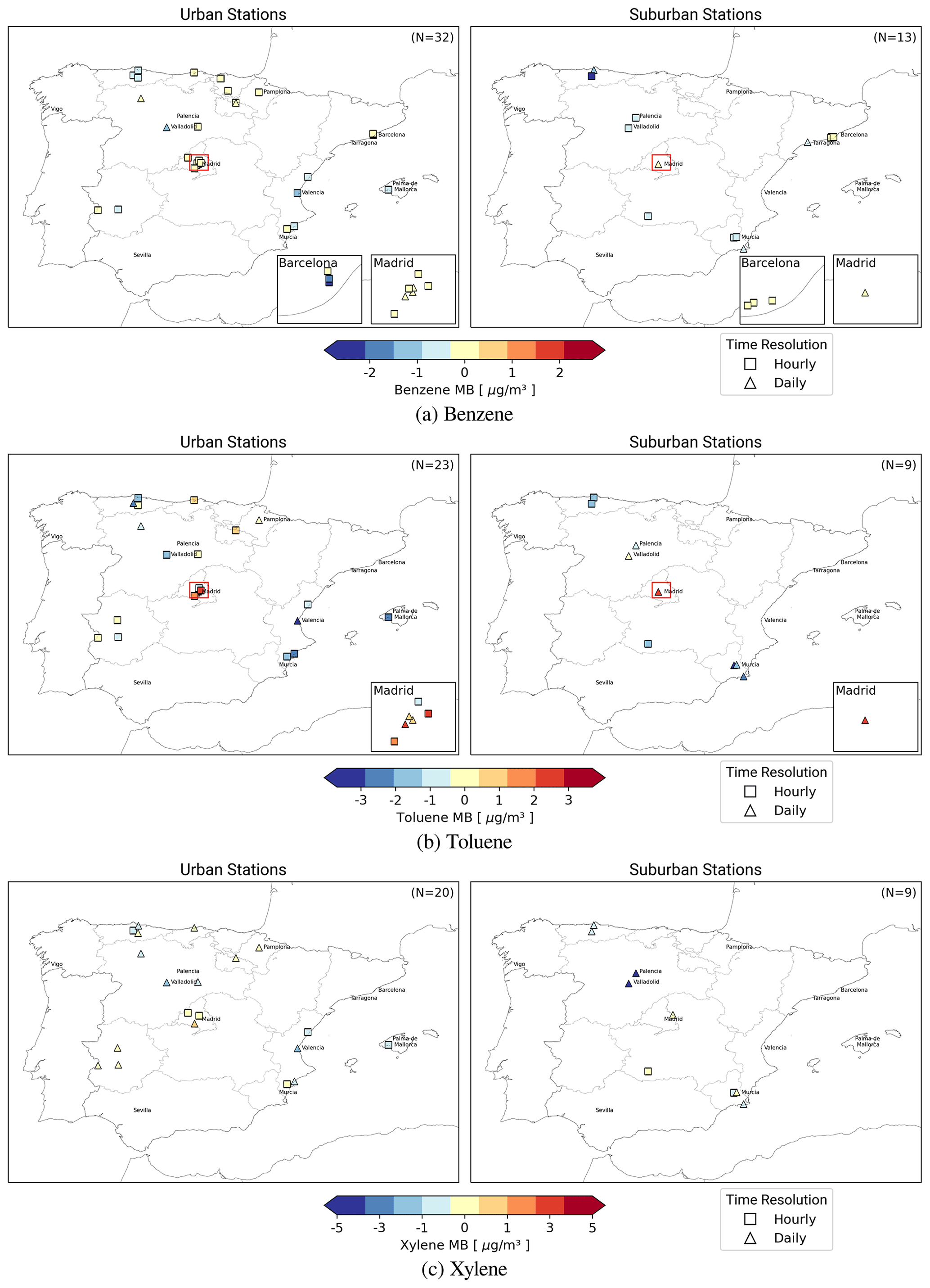
Figure E1Annual mean bias (MB) (µg m−3) between observed and modelled concentrations at urban (left) and suburban stations (right) in 2019 for (a) benzene, (b) toluene, and (c) xylene.
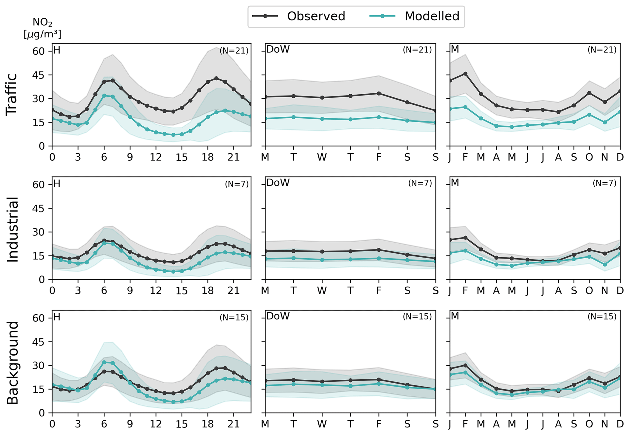
Figure F1Observed (black line) and modelled (blue line) NO2 hourly (H), weekly (day of the week, DoW), and monthly (M) cycles (µg m−3) per station classification for stations also measuring VOCs. The shaded region corresponds to the standard deviation variability.
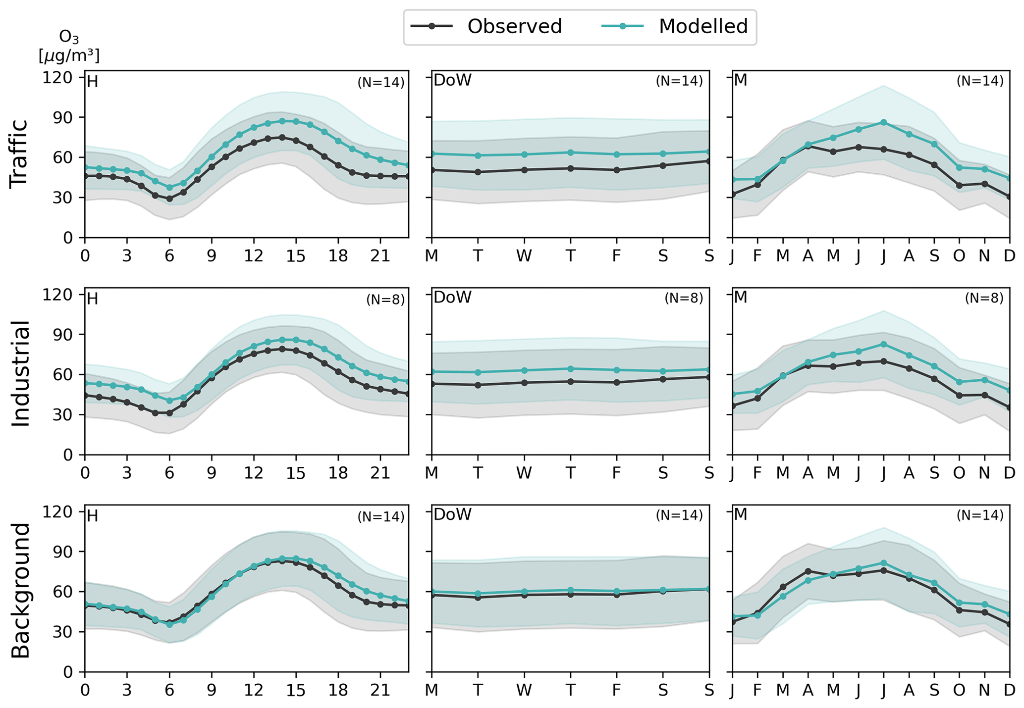
Figure F2Observed (black line) and modelled (blue line) O3 hourly (H), weekly (day of the week, DoW), and monthly (M) cycles (µg m−3) per station classification for stations also measuring VOCs. The shaded region corresponds to the standard deviation variability.
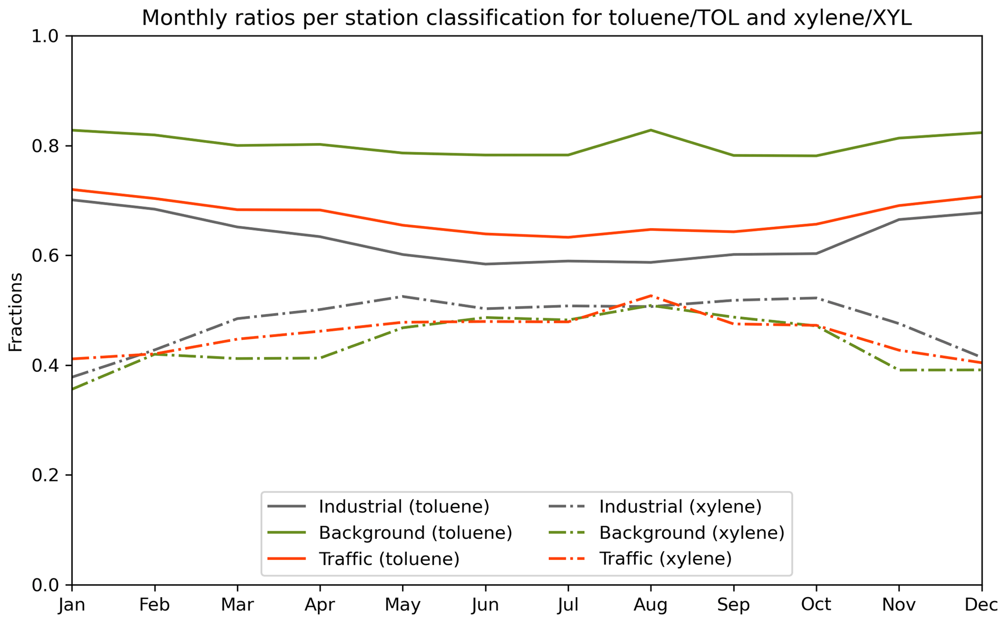
Figure G1Monthly ratios (expressed as fractions) of explicit toluene in lumped species TOL and xylene in lumped species XYL per station classification.
The tables in this appendix provide detailed information about each station, including the measurement methods employed. The following abbreviations are used to denote different measurement techniques: gas chromatography (GC), mass spectrometry (MS), flame ionisation detection (FID), photoionisation detection (PID), and if the method is unknown (UNK).
H1 Stations measuring benzene
Table H1Location and characteristics of selected stations measuring benzene in 2019.
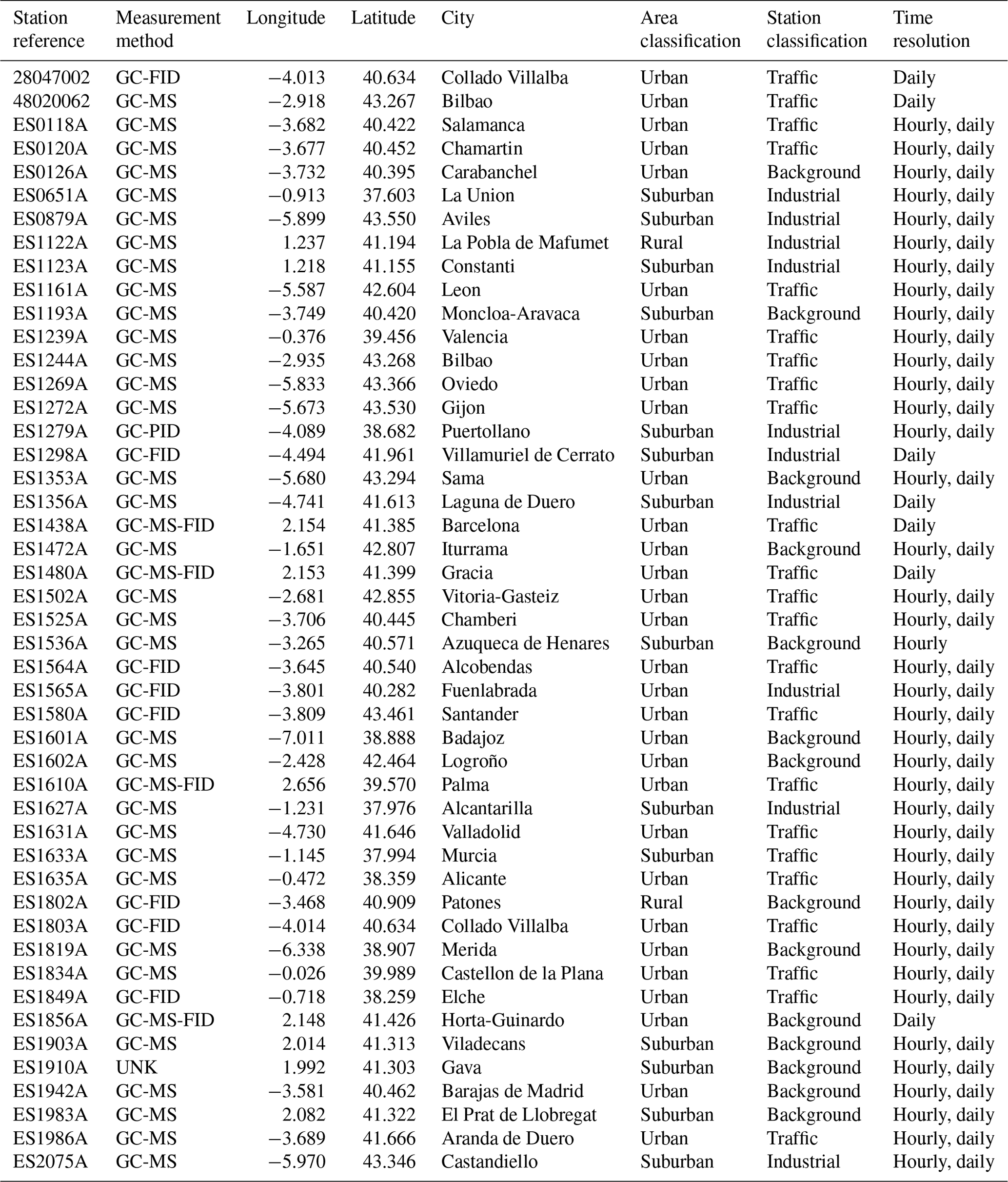
H2 Stations measuring toluene
Table H2Location and characteristics of selected stations measuring toluene in 2019.
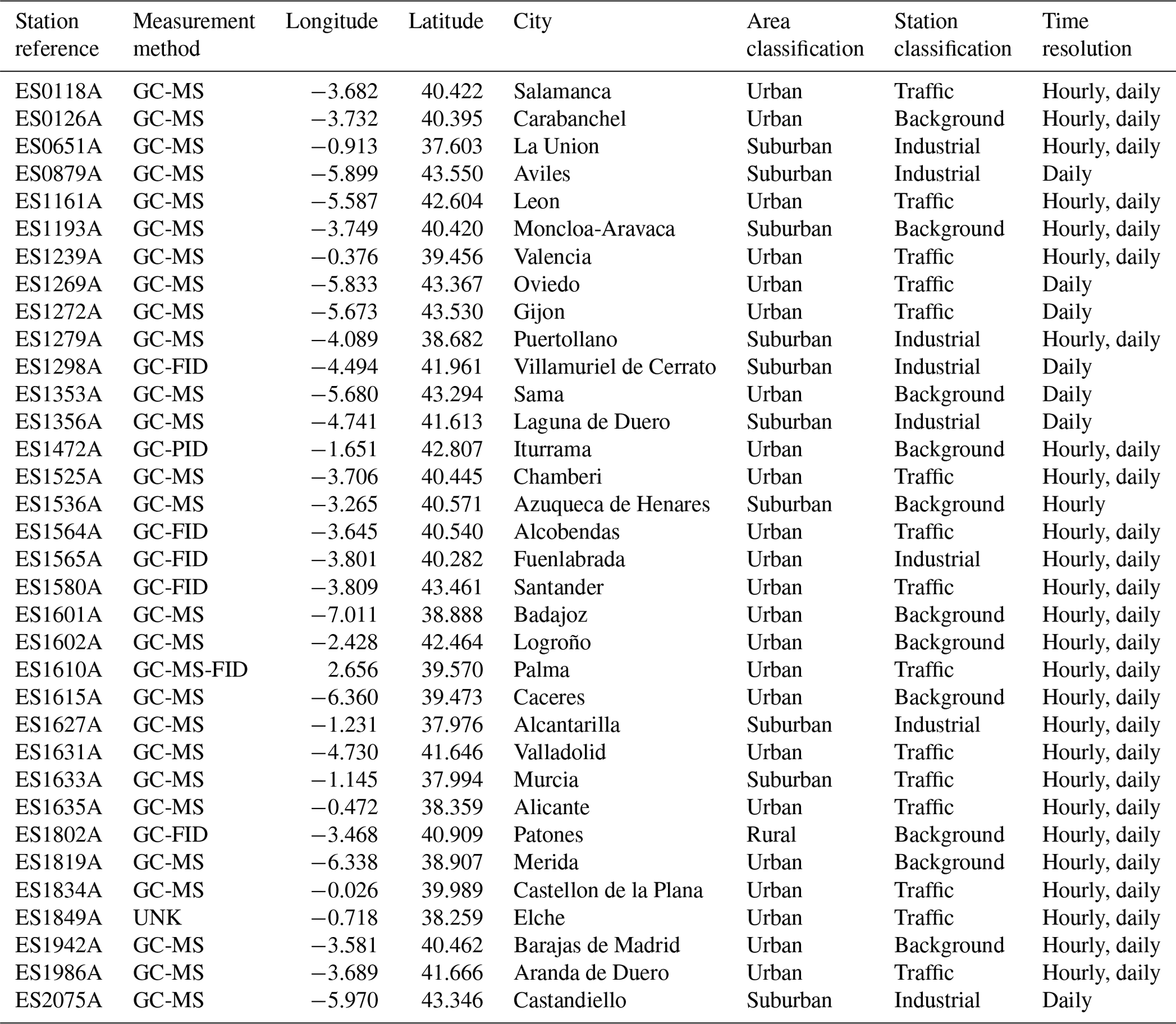
H3 Stations measuring xylene
Table H3Location and characteristics of selected stations measuring xylene in 2019.
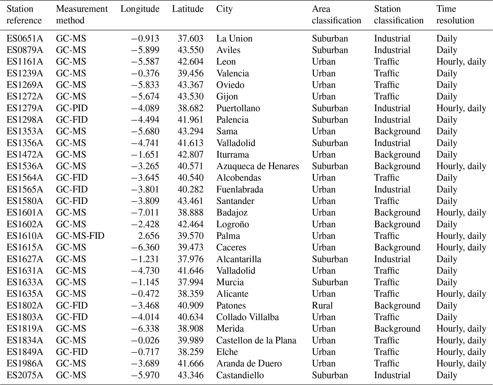
I1 Industrial
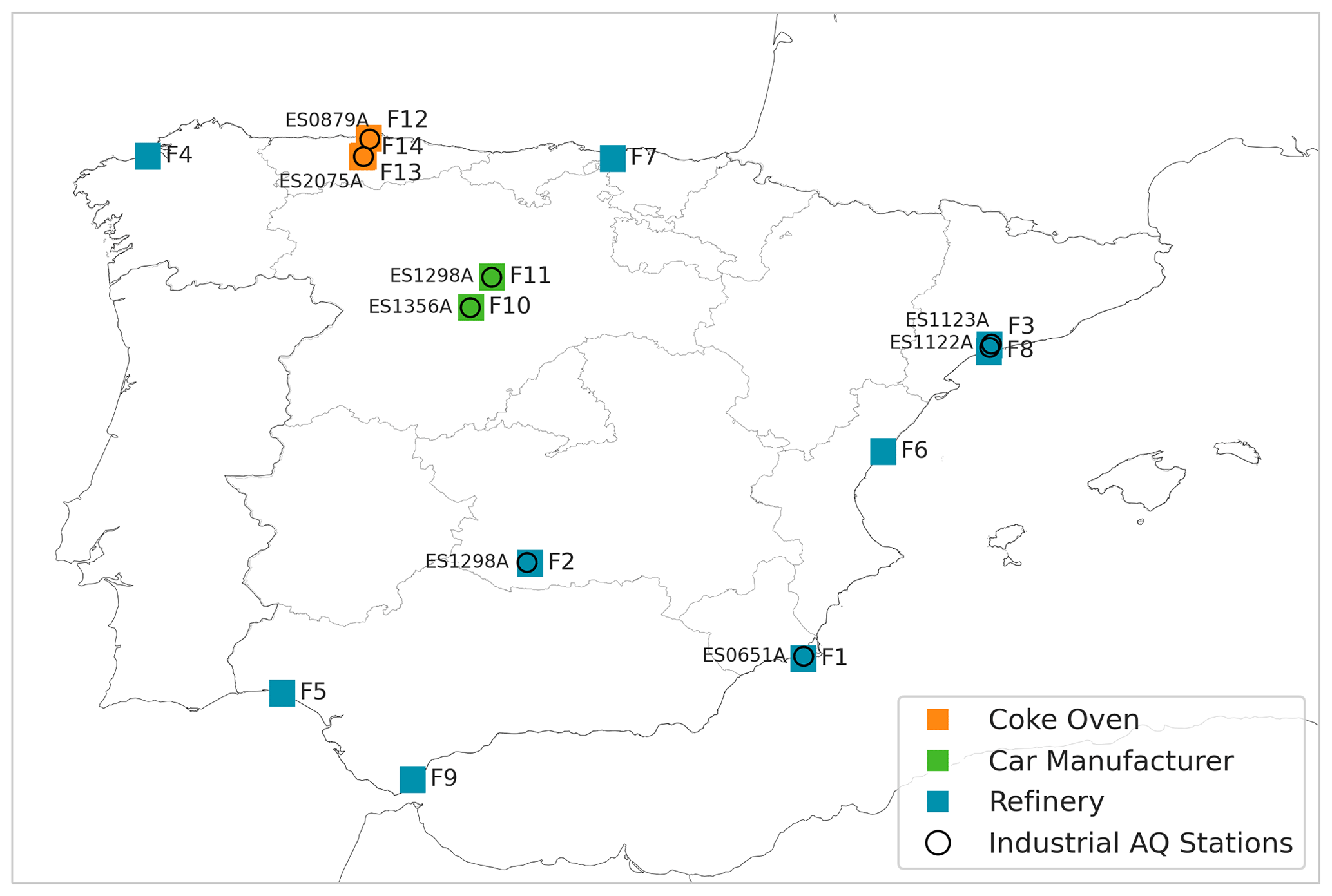
Figure I1Location of the industrial AQ stations and the facilities accounting for the industrial sensitivity analysis, with the respective HERMESv3 code.
I2 Mopeds and motorcycles
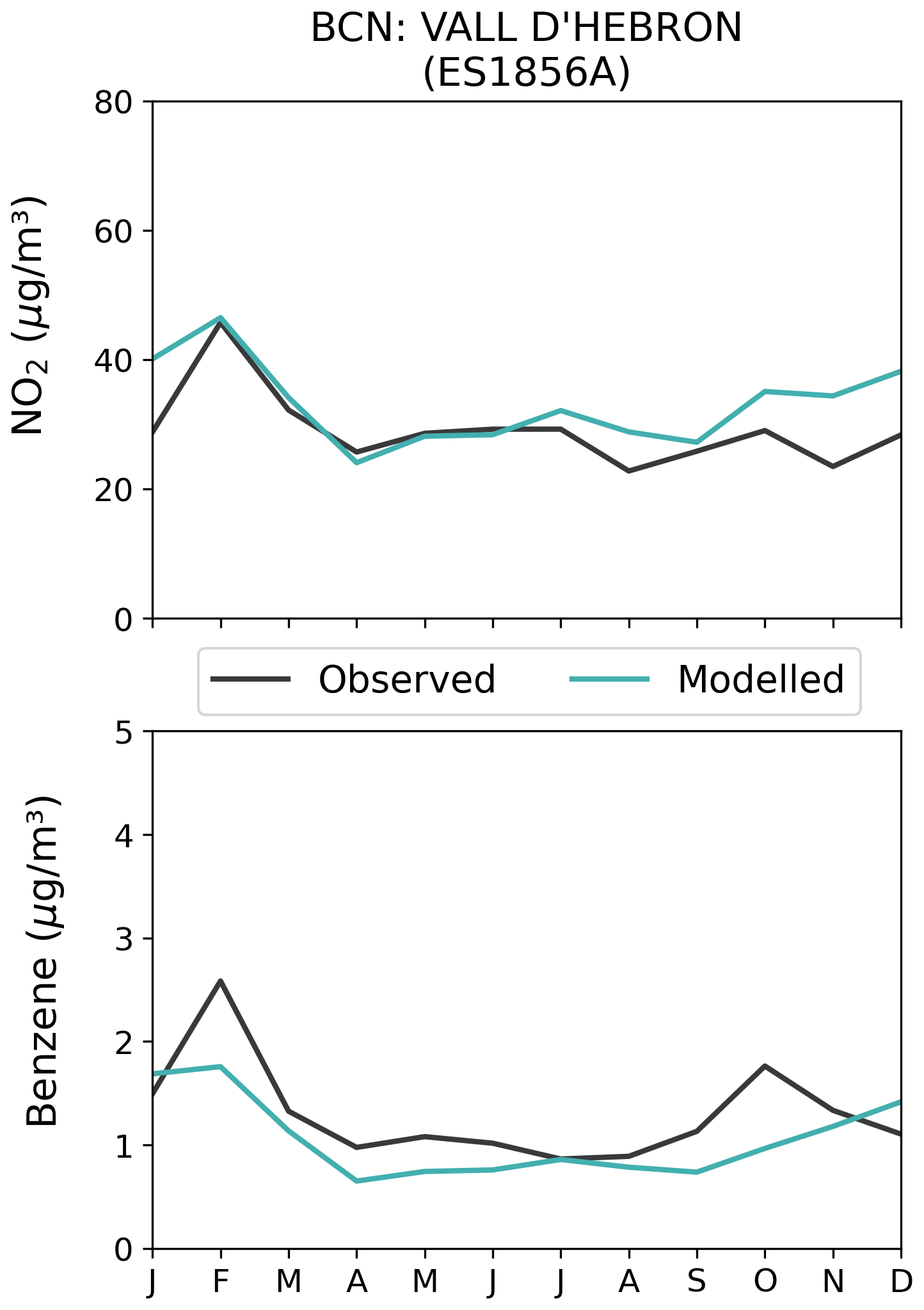
Figure I2Monthly NO2 and benzene concentrations (µg m−3) at the urban background station ES1856A in Barcelona (BCN).
Table I1Data used to estimate correction factors accounting for different vehicle categories ages. Mcorr is the mileage correction factor for a given mileage, Mmean is the mean fleet mileage of vehicles for which the correction is applied, AM is the degradation of the emission performance per kilometre, and BM is the emission level of a fleet of brand new vehicles, which is assumed to be 1.
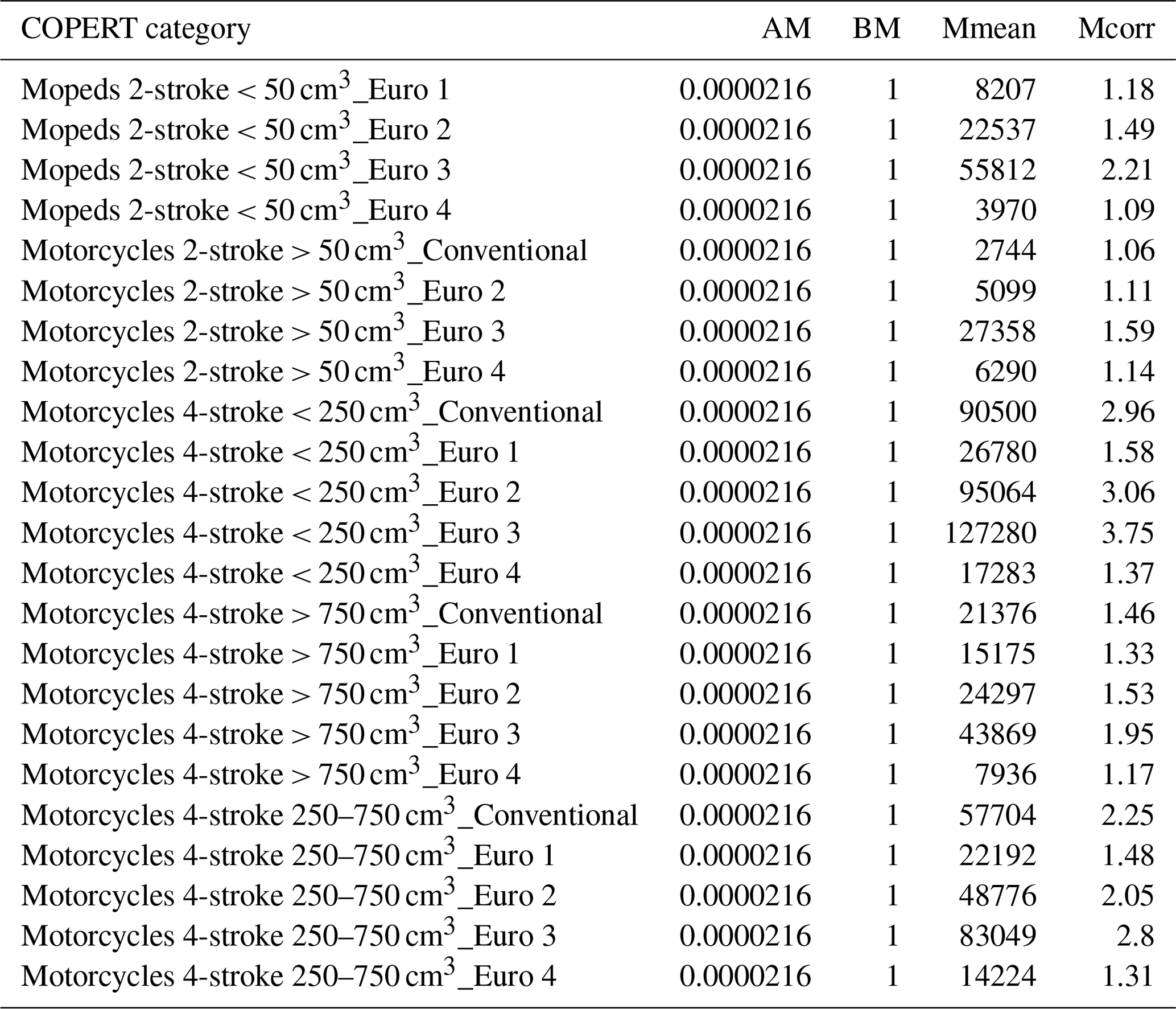
The HERMESv3_BU code package is accessible through the GitLab repository: https://earth.bsc.es/gitlab/es/hermesv3_bu (last access: 16 November 2023) (https://doi.org/10.5281/zenodo.3521897, Guevara et al., 2019a). The MONARCH source code used in this work is accessible through the GitLab repository: https://earth.bsc.es/gitlab/es/monarch (last access: 16 November 2023) (https://doi.org/10.5281/zenodo.5215467, Klose et al., 2021b). Both repositories have a wiki with the model instructions.
The dataset used in this work is available publicly here: https://doi.org/10.5281/zenodo.10637449 (Bowdalo, 2024). The dataset is fully described here: https://doi.org/10.5194/essd-2023-397.
KO: conceptualisation, investigation, data curation, methodology, and writing. MG: conceptualisation, investigation, supervision, data curation, methodology, and writing. OJ: funding acquisition, supervision, software, methodology, and writing and reviewing. HP: methodology, software, and writing and reviewing. DB: methodology and data curation. CT: software. GMP: software. FL: software. CPGP: supervision, funding acquisition, project administration, and reviewing.
The contact author has declared that none of the authors has any competing interests.
Publisher’s note: Copernicus Publications remains neutral with regard to jurisdictional claims made in the text, published maps, institutional affiliations, or any other geographical representation in this paper. While Copernicus Publications makes every effort to include appropriate place names, the final responsibility lies with the authors.
The research leading to these results has received funding from the Ministerio para la Transición Ecológica y el Reto Demográfico (MITECO) as part of the Plan Nacional del Ozono project (grant nos. BOE-A-2021-20183, BOE-A-2023-24403); the Ministerio de Ciencia, Innovación y Universidades (MICINN) as part of the BROWNING project (grant no. RTI2018-099894-B-I00 funded by MCIN/AEI/10.13039/501100011033 and by ERDF “A way of making Europe”); the VITALISE project (grant no. PID2019-108086RA-I00 funded by MCIN/AEI/10.13039/501100011033); the MITIGATE project (grant no. PID2020-113840RA-I00 funded by MCIN/AEI/10.13039/501100011033); the Ramon y Cajal grant (RYC2021-034511-I, MCIN/AEI/10.13039/501100011033 and European Union NextGenerationEU/PRTR); the Red Temática ACTRIS España (grant no. CGL2017-90884-REDT); the AXA Research Fund; and the European Research Council (grant no. 773051, FRAGMENT). K. Oliveira acknowledges the support received from grant PRE2020-092616 funded by MCIN/AEI/10.13039/501100011033 and ESF “Investing in your Future”. BSC also acknowledges the computer resources at MareNostrum and the technical support provided by the Barcelona Supercomputing Center through the RES (grant nos. AECT-2022-2-0003, AECT-2023-3-0018). The authors also thank the four anonymous reviewers for their constructive feedback, which helped improve the quality of the paper.
This research has been supported by the Ministerio para la Transición Ecológica y el Reto Demográfico (grant nos. BOE-A-2021-20183 and BOE-A-2023-24403), the Ministerio de Ciencia e Innovación (grant nos. RTI2018-099894-B-I00, PID2019-108086RA-I00, CGL2017-90884-REDT, and MCIN/AEI/10.13039/501100011033), the European Research Council H2020 (grant no. 773051), the Ramon y Cajal grant MCIN/AEI/10.13039/501100011033 (grant no. RYC2021-034511-I), the European Union NextGenerationEU/PRTR, the AXA Research Fund (grant no. AXA Research Fund), MCIN/AEI/10.13039/501100011033 and ESF “Investing in your Future” (grant no. PRE2020-092616), and the RES (grant nos. AECT-2022-2-0003 and AECT-2023-3-0018).
This paper was edited by Leiming Zhang and reviewed by four anonymous referees.
Adam, T., Farfaletti, A., Montero, L., Martini, G., Manfredi, U., Larsen, B., Santi, G. D., Krasenbrink, A., and Astorga, C.: Chemical characterization of emissions from modern two-stroke mopeds complying with legislative regulation in Europe (EURO-2), Environ. Sci. Technol., 44, 505–512, 2010. a
Agency, E. E.: The Application of Models Under the European Union's Air Quality Directive: A Technical Reference Guide, Publications Office of the European Union, https://doi.org/10.2800/80600, 2011. a
Air Quality Expert Group: Non-methane Volatile Organic Compounds in the UK, https://uk-air.defra.gov.uk/assets/documents/reports/cat09/2006240803_Non_Methane_Volatile_Organic_Compounds_in_the_UK.pdf, (last access: 31 July 2023), 2020. a
Alford, K. L. and Kumar, N.: Pulmonary health effects of indoor volatile organic compounds – a meta-analysis, Int. J. Env. Res. Pub. He., 18, 1578, https://doi.org/10.3390/ijerph18041578, 2021. a
Aries, E., Ciaparra, D., Schofield, M., Anderson, D., Schofield, N., and Fisher, R.: Fugitive and stationary source emissions from coke plants and impact on the local ambient air quality, Year-Book Coke Oven Manag. Assoc. UK, 136–197, http://www.inchiostroverde.it/wp-content/uploads/2012/07/coke.pdf, (last access: 18 June 2024), 2007. a, b, c
Atkinson, R. and Arey, J.: Atmospheric degradation of volatile organic compounds, Chem. Rev., 103, 4605–4638, 2003. a
Atkinson, R., Aschmann, S. M., Arey, J., and Carter, W. P.: Formation of ring-retaining products from the OH radical-initiated reactions of benzene and toluene, Int. J. Chem. Kinet., 21, 801–827, 1989. a
Badia, A. and Jorba, O.: Gas-phase evaluation of the online NMMB/BSC-CTM model over Europe for 2010 in the framework of the AQMEII-Phase2 project, Atmos. Environ., 115, 657–669, 2015. a
Badia, A., Jorba, O., Voulgarakis, A., Dabdub, D., Pérez García-Pando, C., Hilboll, A., Gonçalves, M., and Janjic, Z.: Description and evaluation of the Multiscale Online Nonhydrostatic AtmospheRe CHemistry model (NMMB-MONARCH) version 1.0: gas-phase chemistry at global scale, Geosci. Model Dev., 10, 609–638, https://doi.org/10.5194/gmd-10-609-2017, 2017. a, b
Baltensperger, U., Kalberer, M., Dommen, J., Paulsen, D., Alfarra, M. R., Coe, H., Fisseha, R., Gascho, A., Gysel, M., Nyeki, S., Sax, M., Steinbacher, M., Prevot, A. S. H., Sjögren, S., Weingartner, E., and Zenobi, R.: Secondary organic aerosols from anthropogenic and biogenic precursors, Faraday Discuss., 130, 265–278, 2005. a
Bates, K. H., Jacob, D. J., Li, K., Ivatt, P. D., Evans, M. J., Yan, Y., and Lin, J.: Development and evaluation of a new compact mechanism for aromatic oxidation in atmospheric models, Atmos. Chem. Phys., 21, 18351–18374, https://doi.org/10.5194/acp-21-18351-2021, 2021. a
Bayliss, D., Chen, C., Jarabek, A., Sonawane, B., and Valcovic, L.: Carcinogenic effects of benzene: an update, U.S. Environmental Protection Agency, Office of Research and Development, National Center for Environmental Assessment, Washington Office, Washington, DC, EPA/600/P-97/001F, 1998. a
Borbon, A., Boynard, A., Salameh, T., Baudic, A., Gros, V., Gauduin, J., Perrussel, O., and Pallares, C.: Is traffic still an important emitter of monoaromatic organic compounds in European urban areas?, Environ. Sci. Technol., 52, 513–521, 2018. a
Bowdalo, D.: GHOST: A globally harmonised dataset of surface atmospheric composition measurements (1.5), Zenodo [data set], https://doi.org/10.5281/zenodo.10637450, 2024. a
Bowdalo, D., Basart, S., Guevara, M., Jorba, O., Pérez García-Pando, C., Jaimes Palomera, M., Rivera Hernandez, O., Puchalski, M., Gay, D., Klausen, J., Moreno, S., Netcheva, S., and Tarasova, O.: GHOST: A globally harmonised dataset of surface atmospheric composition measurements, Earth Syst. Sci. Data Discuss. [preprint], https://doi.org/10.5194/essd-2023-397, in review, 2024. a
Brunner, D., Savage, N., Jorba, O., Eder, B., Giordano, L., Badia, A., Balzarini, A., Baró, R., Bianconi, R., Chemel, C., Curci, G., Forkel, R., Jiménez-Guerrero, P., Hirtl, M., Hodzic, A., Honzak, L., Im, U., Knote, C., Makar, P., Manders-Groot, A., van Meijgaard, E., Neal, L., Pérez, J. L., Pirovano, G., San Jose, R., Schröder, W., Sokhi, R. S., Syrakov, D., Torian, A., Tuccella, P., Werhahn, J., Wolke, R., Yahya, K., Zabkar, R., Zhang, Y., Hogrefe, C., and Galmarini, S.: Comparative analysis of meteorological performance of coupled chemistry-meteorology models in the context of AQMEII phase 2, Atmos. Environ., 115, 470–498, https://doi.org/10.1016/j.atmosenv.2014.12.032, 2015. a
Byun, D. and Ching, J.: Science algorithms of the EPA models-3 community multiscale air quality model (CMAQ) modeling system, Rep.EPA/600/R-99, U.S. Environmental Protection Agency, Office of Research and Development, 1999. a
Carter, W. P.: A detailed mechanism for the gas-phase atmospheric reactions of organic compounds, Atmos. Environ. Pt. A., 24, 481–518, https://doi.org/10.1016/0960-1686(90)90005-8, 1990. a
Castell, N., Stein, A., Salvador, R., Mantilla, E., and Millán, M.: The impact of biogenic VOC emissions on photochemical ozone formation during a high ozone pollution episode in the Iberian Peninsula in the 2003 summer season, Adv. Sci. Res., 2, 9–15, 2008. a
Chen, T., Zhang, P., Chu, B., Ma, Q., Ge, Y., Liu, J., and He, H.: Secondary organic aerosol formation from mixed volatile organic compounds: Effect of RO2 chemistry and precursor concentration, npj Clim. Atmos. Sci., 5, 95, https://doi.org/10.1038/s41612-022-00321-y, 2022. a
Cui, L., Wu, D., Wang, S., Xu, Q., Hu, R., and Hao, J.: Measurement report: Ambient volatile organic compound (VOC) pollution in urban Beijing: characteristics, sources, and implications for pollution control, Atmos. Chem. Phys., 22, 11931–11944, https://doi.org/10.5194/acp-22-11931-2022, 2022. a
Dallmann, T., Bernard, Y., Tietge, U., and Muncrief, R.: Remote sensing of motor vehicle emissions in Paris, The Real Urban Emissions Initiative: London, UK, https://theicct.org/wp-content/uploads/2021/06/TRUE_ParisRS_study_20190909.pdf, (last access: 18 June 2024), 2019. a
Day, M., Pouliot, G., Hunt, S., Baker, K. R., Beardsley, M., Frost, G., Mobley, D., Simon, H., Henderson, B. B., Yelverton, T., and Rao, V.: Reflecting on progress since the 2005 NARSTO emissions inventory report, J. Air Waste Manag. Assoc., 69, 1023–1048, 2019. a
EC: Directive 2008/50/EC of the European Parliament and of the Council of 21 May 2008 on ambient air quality and cleaner air for Europe, Official Journal of the European Union, 1–44, 2008. a, b
EEA: EMEP/EEA air pollutant emission inventory guidebook 2019: 2.D.3.d Coating applications, https://www.eea.europa.eu/publications/emep-eea-guidebook-2019/, (last access: 4 September 2023), 2019. a
EEA: EMEP/EEA air pollutant emission inventory guidebook 2016: 1.A.3.b.i-iv Road transport, https://www.eea.europa.eu/publications/, (last access: 18 June 2024), 2016. a
EEA: Air Quality e-Reporting database, https://www.eea.europa.eu/en/datahub/datahubitem-view/3b390c9c-f321-490a-b25a-ae93b2ed80c1, (last access: 20 September 2023), 2023. a
Filley, C. M., Halliday, W., and Kleinschmidt-Demasters, B. K.: The Effects of Toluene on the Central Nervous System, J. Neuropathol. Exp. Neurol., 63, 1–12, https://doi.org/10.1093/jnen/63.1.1, 2004. a
Flemming, J., Huijnen, V., Arteta, J., Bechtold, P., Beljaars, A., Blechschmidt, A.-M., Diamantakis, M., Engelen, R. J., Gaudel, A., Inness, A., Jones, L., Josse, B., Katragkou, E., Marecal, V., Peuch, V.-H., Richter, A., Schultz, M. G., Stein, O., and Tsikerdekis, A.: Tropospheric chemistry in the Integrated Forecasting System of ECMWF, Geosci. Model Dev., 8, 975–1003, https://doi.org/10.5194/gmd-8-975-2015, 2015. a
Foley, K. M., Roselle, S. J., Appel, K. W., Bhave, P. V., Pleim, J. E., Otte, T. L., Mathur, R., Sarwar, G., Young, J. O., Gilliam, R. C., Nolte, C. G., Kelly, J. T., Gilliland, A. B., and Bash, J. O.: Incremental testing of the Community Multiscale Air Quality (CMAQ) modeling system version 4.7, Geosci. Model Dev., 3, 205–226, https://doi.org/10.5194/gmd-3-205-2010, 2010. a
Franco, B., Clarisse, L., Van Damme, M., Hadji-Lazaro, J., Clerbaux, C., and Coheur, P.-F.: Ethylene industrial emitters seen from space, Nat. Commun., 13, 6452, https://doi.org/10.1038/s41467-022-34098-8, 2022. a
Gallego-Díez, M. L., Correa-Ochoa, M. A., and Saldarriaga-Molina, J. C.: Validation of a methodology to determine Benzene, Toluene, Ethylbenzene, and Xylenes concentration present in the air and adsorbed in activated charcoal passive samplers by GC/FID chromatography, Revista Facultad de Ingeniería Universidad de Antioquia, 138–149, ISSN: 0120-6230, https://www.redalyc.org/articulo.oa?id=43045911013 (last access: 13 November 2023), 2016. a
Ge, Y., Solberg, S., Heal, M., Reimann, S., van Caspel, W., Hellack, B., Salameh, T., and Simpson, D.: Evaluation of modelled versus observed NMVOC compounds at EMEP sites in Europe, EGUsphere [preprint], https://doi.org/10.5194/egusphere-2023-3102, 2024. a
Georgiou, G. K., Christoudias, T., Proestos, Y., Kushta, J., Pikridas, M., Sciare, J., Savvides, C., and Lelieveld, J.: Evaluation of WRF-Chem model (v3.9.1.1) real-time air quality forecasts over the Eastern Mediterranean, Geosci. Model Dev., 15, 4129–4146, https://doi.org/10.5194/gmd-15-4129-2022, 2022. a
Gery, M. W., Whitten, G. Z., Killus, J. P., and Dodge, M. C.: A photochemical kinetics mechanism for urban and regional scale computer modeling, J. Geophys. Res.-Atmos., 94, 12925–12956, 1989. a, b
Guenther, A., Karl, T., Harley, P., Wiedinmyer, C., Palmer, P. I., and Geron, C.: Estimates of global terrestrial isoprene emissions using MEGAN (Model of Emissions of Gases and Aerosols from Nature), Atmos. Chem. Phys., 6, 3181–3210, https://doi.org/10.5194/acp-6-3181-2006, 2006. a, b
Guenther, A. B., Jiang, X., Heald, C. L., Sakulyanontvittaya, T., Duhl, T., Emmons, L. K., and Wang, X.: The Model of Emissions of Gases and Aerosols from Nature version 2.1 (MEGAN2.1): an extended and updated framework for modeling biogenic emissions, Geoscientific Model Development, pp. 1471–1492, https://doi.org/10.5194/gmd-12-1885-2019, 2012. a
Guevara, M., Medina, C. T., Jorba, O., and García-Pando, C. P.: HERMESv3_BU model, Zenodo [code], https://doi.org/10.5281/zenodo.3521897, 2019a. a
Guevara, M., Tena, C., Porquet, M., Jorba, O., and Pérez García-Pando, C.: HERMESv3, a stand-alone multi-scale atmospheric emission modelling framework – Part 1: global and regional module, Geosci. Model Dev., 12, 1885–1907, https://doi.org/10.5194/gmd-12-1885-2019, 2019. b. a, b
Guevara, M., Tena, C., Porquet, M., Jorba, O., and Pérez García-Pando, C.: HERMESv3, a stand-alone multi-scale atmospheric emission modelling framework – Part 2: The bottom–up module, Geosci. Model Dev., 13, 873–903, https://doi.org/10.5194/gmd-13-873-2020, 2020. a, b, c, d
Guevara, M., Petetin, H., Jorba, O., Denier van der Gon, H., Kuenen, J., Super, I., Granier, C., Doumbia, T., Ciais, P., Liu, Z., Lamboll, R. D., Schindlbacher, S., Matthews, B., and Pérez García-Pando, C.: Towards near-real-time air pollutant and greenhouse gas emissions: lessons learned from multiple estimates during the COVID-19 pandemic, Atmos. Chem. Phys., 23, 8081–8101, https://doi.org/10.5194/acp-23-8081-2023, 2023. a
Henrot, A.-J., Stanelle, T., Schröder, S., Siegenthaler, C., Taraborrelli, D., and Schultz, M. G.: Implementation of the MEGAN (v2.1) biogenic emission model in the ECHAM6-HAMMOZ chemistry climate model, Geosci. Model Dev., 10, 903–926, https://doi.org/10.5194/gmd-10-903-2017, 2017. a
Huang, R.-J., Zhang, Y., Bozzetti, C., Ho, K.-F., Cao, J.-J., Han, Y., Daellenbach, K. R., Slowik, J. G., Platt, S. M., Canonaco, F., Zotter, P., Wolf, R., Pieber, S. M., Bruns, E. A., Crippa, M., Ciarelli, G., Piazzalunga, A., Schwikowski, M., Abbaszade, G., Schnelle-Kreis, J., Zimmermann, R., An, Z., Szidat, S., Baltensperger, U., Haddad, I. E., and Prévôt, A. S. H.: High secondary aerosol contribution to particulate pollution during haze events in China, Nature, 514, 218–222, 2014. a
INE: Instituto Nacional de Estadística, Cifras de Población Censo 2021, https://www.ine.es/jaxi/Datos.htm?tpx=55198 (last access: 28 March 2023), 2021. a
In’t Veld, M., Seco, R., Reche, C., Pérez, N., Alastuey, A., Portillo- Estrada, M., Janssens, I. A., Peñuelas, J., Fernandez-Martinez, M., Marchand, N., Temime-Roussel, B., Querol, X., and Yáñez-Serrano, A. M.: Identification of volatile organic compounds and their sources driving ozone and secondary organic aerosol formation in NE Spain, Sci. Total Environ., 906, 167159, https://doi.org/10.1016/j.scitotenv.2023.167159, 2024. a, b
Janjic, Z. and Gall, I.: Scientific documentation of the NCEP nonhydrostatic multiscale model on the B grid (NMMB), Part 1: Dynamics, Tech. rep., NCAR/TN-489+STR, https://doi.org/10.5065/D6WH2MZX, 2012. a
Jookjantra, P., Thepanondh, S., Keawboonchu, J., Kultan, V., and Laowagul, W.: Formation potential and source contribution of secondary organic aerosol from volatile organic compounds, Tech. rep., Wiley Online Library, Journal of Environmental Quality, https://doi.org/10.1002/jeq2.20381, 2022. a
Kanakidou, M., Tsigaridis, K., Dentener, F. J., and Crutzen, P. J.: Human-activity-enhanced formation of organic aerosols by biogenic hydrocarbon oxidation, J. Geophys. Res.-Atmos., 105, 9243–9354, 2000. a
Kansal, A.: Sources and reactivity of NMHCs and VOCs in the atmosphere: A review, J. Hazard. Mater., 166, 17–26, https://doi.org/10.1016/j.jhazmat.2008.11.048, 2009. a, b
Klose, M., Jorba, O., Gonçalves Ageitos, M., Escribano, J., Dawson, M. L., Obiso, V., Di Tomaso, E., Basart, S., Montané Pinto, G., Macchia, F., Ginoux, P., Guerschman, J., Prigent, C., Huang, Y., Kok, J. F., Miller, R. L., and Pérez García-Pando, C.: Mineral dust cycle in the Multiscale Online Nonhydrostatic AtmospheRe CHemistry model (MONARCH) Version 2.0, Geosci. Model Dev., 14, 6403–6444, https://doi.org/10.5194/gmd-14-6403-2021, 2021a. a, b, c
Klose, M., Jorba, O., Gonçalves Ageitos, M., Escribano, J., Dawson, M. L., Obiso, V., Di Tomaso, E., Basart, S., Montané Pinto, G., Macchia, F., and Pérez García-Pando, C.: MONARCH: Multiscale Online Nonhydrostatic AtmospheRe CHemistry model Version 2.0, Zenodo [code], https://doi.org/10.5281/zenodo.5215467, 2021b. a
Kuenen, J., Dellaert, S., Visschedijk, A., Jalkanen, J.-P., Super, I., and Denier van der Gon, H.: CAMS-REG-v4: a state-of-the-art high-resolution European emission inventory for air quality modelling, Earth Syst. Sci. Data, 14, 491–515, https://doi.org/10.5194/essd-14-491-2022, 2022. a
Le Bras, G.: LACTOZ Publications 1988–1995, in: Chemical Processes in Atmospheric Oxidation: Laboratory Studies of Chemistry Related to Tropospheric Ozone, 257–309, Springer, ISBN : 978-3-642-63902-9, 1997. a
Ling, C., Cui, L., and Li, R.: Global impact of the COVID-19 lockdown on surface concentration and health risk of atmospheric benzene, Atmos. Chem. Phys., 23, 3311–3324, https://doi.org/10.5194/acp-23-3311-2023, 2023. a
Luecken, D., Hutzell, W., Strum, M., and Pouliot, G.: Regional sources of atmospheric formaldehyde and acetaldehyde, and implications for atmospheric modeling, Atmos. Environ., 47, 477–490, 2012. a
MITECO: Estadística mensual de destilación carbones enero a diciembre 2018, https://energia.gob.es/balances/Publicaciones/carbon_mensuales/Paginas/destilacion_carbon.aspx (last access: 4 September 2023), 2019. a
MITERD: Datos oficiales Calidad del Aire 2019, https://www.miteco.gob.es/es/calidad-y-evaluacion-ambiental/ (last access: 29 February 2024), 2020. a
MITERD: Informative Inventory Report. Submission To The Secretariat Of The Geneva Convention And EMEP programme Reporting to the European Commission under Directive (EU) 2016/2284, https://www.miteco.gob.es/content/, (last access: 18 June 2024), 2022. a, b
MITERD: PRTR-Espana: Información pública fuentes puntuales, https://prtr-es.es/Informes/InventarioInstalacionesIPPC.aspx (last access: 17 November 2023), 2023. a
Monks, P. S., Archibald, A. T., Colette, A., Cooper, O., Coyle, M., Derwent, R., Fowler, D., Granier, C., Law, K. S., Mills, G. E., Stevenson, D. S., Tarasova, O., Thouret, V., von Schneidemesser, E., Sommariva, R., Wild, O., and Williams, M. L.: Tropospheric ozone and its precursors from the urban to the global scale from air quality to short-lived climate forcer, Atmos. Chem. Phys., 15, 8889–8973, https://doi.org/10.5194/acp-15-8889-2015, 2015. a
Navarro-Barboza, H., Pandolfi, M., Guevara, M., Enciso, S., Tena, C., Via, M., Yus-Díez, J., Reche, C., Pérez, N., Alastuey, A., Querol, X., and Jorba, O.: Uncertainties in source allocation of carbonaceous aerosols in a Mediterranean region, Environ. Int., 183, 108252, https://doi.org/10.1016/j.envint.2023.108252, 2023. a
Niaz, K., Bahadar, H., Maqbool, F., and Abdollahi, M.: A review of environmental and occupational exposure to xylene and its health concerns, EXCLI J., 14, 1167, https://doi.org/10.17179/excli2015-623, 2015. a
Oliveira, K., Guevara, M., Jorba, O., Querol, X., and García-Pando, C. P.: A new NMVOC speciated inventory for a reactivity-based approach to support ozone control strategies in Spain, Sci. Total Environ., 867, 161449, https://doi.org/10.1016/j.scitotenv.2023.161449, 2023. a, b, c, d, e, f, g, h
Parrish, D. D., Ryerson, T. B., Mellqvist, J., Johansson, J., Fried, A., Richter, D., Walega, J. G., Washenfelder, R. A., de Gouw, J. A., Peischl, J., Aikin, K. C., McKeen, S. A., Frost, G. J., Fehsenfeld, F. C., and Herndon, S. C.: Primary and secondary sources of formaldehyde in urban atmospheres: Houston Texas region, Atmos. Chem. Phys., 12, 3273–3288, https://doi.org/10.5194/acp-12-3273-2012, 2012. a
País, E.: La producción de coches en España, https://cincodias.elpais.com/cincodias/2020/01/23/companias/1579778720_044430.html (last access: 28 July 2023), 2020. a
Petetin, H., Guevara, M., Garatachea, R., López, F., Oliveira, K., Enciso, S., Jorba, O., Querol, X., Massagué, J., Alastuey, A., and Pérez García-Pando, C.: Assessing ozone abatement scenarios in the framework of the Spanish ozone mitigation plan, Sci. Total Environ., 902, 165380, https://doi.org/10.1016/j.scitotenv.2023.165380, 2023. a
Querol, X., Gangoiti, G., Mantilla, E., Alastuey, A., Minguillón, M. C., Amato, F., Reche, C., Viana, M., Moreno, T., Karanasiou, A., Rivas, I., Pérez, N., Ripoll, A., Brines, M., Ealo, M., Pandolfi, M., Lee, H.-K., Eun, H.-R., Park, Y.-H., Escudero, M., Beddows, D., Harrison, R. M., Bertrand, A., Marchand, N., Lyasota, A., Codina, B., Olid, M., Udina, M., Jiménez-Esteve, B., Soler, M. R., Alonso, L., Millán, M., and Ahn, K.-H.: Phenomenology of high-ozone episodes in NE Spain, Atmos. Chem. Phys., 17, 2817–2838, https://doi.org/10.5194/acp-17-2817-2017, 2017. a
Querol, X., Alastuey, A., Gangoiti, G., Perez, N., Lee, H. K., Eun, H. R., Park, Y., Mantilla, E., Escudero, M., Titos, G., Alonso, L., Temime-Roussel, B., Marchand, N., Moreta, J. R., Revuelta, M. A., Salvador, P., Artíñano, B., García dos Santos, S., Anguas, M., Notario, A., Saiz-Lopez, A., Harrison, R. M., Millán, M., and Ahn, K.-H.: Phenomenology of summer ozone episodes over the Madrid Metropolitan Area, central Spain, Atmos. Chem. Phys., 18, 6511–6533, https://doi.org/10.5194/acp-18-6511-2018, 2018. a
Rodriguez-Rey, D., Guevara, M., Linares, M. P., Casanovas, J., Armengol, J. M., Benavides, J., Soret, A., Jorba, O., Tena, C., and García-Pando, C. P.: To what extent the traffic restriction policies applied in Barcelona city can improve its air quality?, Sci. Total Environ., 807, 150743, https://doi.org/10.1016/j.scitotenv.2021.150743, 2022. a
Russell, A. and Dennis, R.: NARSTO critical review of photochemical models and modeling, Atmos. Environ., 34, 2283–2324, 2000. a
Sarwar, G., Simon, H., Bhave, P., and Yarwood, G.: Examining the impact of heterogeneous nitryl chloride production on air quality across the United States, Atmos. Chem. Phys., 12, 6455–6473, https://doi.org/10.5194/acp-12-6455-2012, 2012. a, b, c
Saxer, C. J., Forss, A.-M., Rüdy, C., and Heeb, N. V.: Benzene, toluene and C2-benzene emissions of 4-stroke motorbikes: Benefits and risks of the current TWC technology, Atmos. Environ., 40, 6053–6065, 2006. a
Schiavina, M., Melchiorri, M., and Pesaresi, M.: GHS-SMOD R2023A – GHS settlement layers, application of the Degree of Urbanisation methodology (stage I) to GHS-POP R2023A and GHS-BUILT-S R2023A, multitemporal (1975–2030). European Commission, Joint Research Centre (JRC), http://data.europa.eu/89h/a0df7a6f-49de-46ea-9bde-563437a6e2ba (last access: 25 October 2023), 2023. a
Scorrano, M. and Danielis, R.: The characteristics of the demand for electric scooters in Italy: An exploratory study, Res. Transp. Busin. Manag., 39, 100589, https://doi.org/10.1016/j.rtbm.2020.100589, 2021. a
She, Y., Li, J., Lyu, X., Guo, H., Qin, M., Xie, X., Gong, K., Ye, F., Mao, J., Huang, L., and Hu, J.: Current status of model predictions on volatile organic compounds and impacts on surface ozone predictions during summer in China, EGUsphere [preprint], https://doi.org/10.5194/egusphere-2023-1358, 2023. a, b
Shuai, J., Kim, S., Ryu, H., Park, J., Lee, C. K., Kim, G.-B., Ultra, V. U., and Yang, W.: Health risk assessment of volatile organic compounds exposure near Daegu dyeing industrial complex in South Korea, BMC Public Health, 18, 1–13, 2018. a
Sicard, M., Jorba, O., Ho, J. J., Izquierdo, R., De Linares, C., Alarcón, M., Comerón, A., and Belmonte, J.: Measurement report: Characterization of the vertical distribution of airborne Pinus pollen in the atmosphere with lidar-derived profiles – a modeling case study in the region of Barcelona, NE Spain, Atmos. Chem. Phys., 21, 17807–17832, https://doi.org/10.5194/acp-21-17807-2021, 2021. a
Skoulidou, I., Koukouli, M.-E., Manders, A., Segers, A., Karagkiozidis, D., Gratsea, M., Balis, D., Bais, A., Gerasopoulos, E., Stavrakou, T., van Geffen, J., Eskes, H., and Richter, A.: Evaluation of the LOTOS-EUROS NO2 simulations using ground-based measurements and S5P/TROPOMI observations over Greece, Atmos. Chem. Phys., 21, 5269–5288, https://doi.org/10.5194/acp-21-5269-2021, 2021. a
Spada, M.: Development and evaluation of an atmospheric aerosol module implemented within the NMMB/BSC-CTM, Ph.D. Thesis, Universitat Politècnica de Catalunya, https://doi.org/10.5821/dissertation-2117-95991, 2015. a
Srivastava, D., Vu, T. V., Tong, S., Shi, Z., and Harrison, R. M.: Formation of secondary organic aerosols from anthropogenic precursors in laboratory studies, npj Clim. Atmos. Sci., 5, 22, https://doi.org/10.1038/s41612-022-00238-6, 2022. a
Steinbacher, M., Zellweger, C., Schwarzenbach, B., Bugmann, S., Buchmann, B., Ordóñez, C., Prévôt, A. S., and Hueglin, C.: Nitrogen oxide measurements at rural sites in Switzerland: Bias of conventional measurement techniques, J. Geophys. Res.-Atmos., 112, D11307, https://doi.org/10.1029/2006JD007971, 2007. a
Sun, J., Wu, F., Hu, B., Tang, G., Zhang, J., and Wang, Y.: VOC characteristics, emissions and contributions to SOA formation during hazy episodes, Atmos. Environ., 141, 560–570, 2016. a
Tagiyeva, N. and Sheikh, A.: Domestic exposure to volatile organic compounds in relation to asthma and allergy in children and adults, Exp. Rev. Clin. Immunol., 10, 1611–1639, 2014. a
Travis, K. R., Nault, B. A., Crawford, J. H., Bates, K. H., Blake, D. R., Cohen, R. C., Fried, A., Hall, S. R., Huey, L. G., Lee, Y. R., Meinardi, S., Min, K.-E., Simpson, I. J., and Ullman, K.: Impact of improved representation of VOC emissions and production of NOx reservoirs on modeled urban ozone production, EGUsphere [preprint], https://doi.org/10.5194/egusphere-2024-951, 2024. a
Tsai, J.-H., Yao, Y.-C., Huang, P.-H., and Chiang, H.-L.: Fuel economy and volatile organic compound exhaust emission for motorcycles with various running mileages, Aerosol Air Qual. Res., 18, 3056–3067, 2018. a
Villena, G., Bejan, I., Kurtenbach, R., Wiesen, P., and Kleffmann, J.: Interferences of commercial NO2 instruments in the urban atmosphere and in a smog chamber, Atmos. Meas. Tech., 5, 149–159, https://doi.org/10.5194/amt-5-149-2012, 2012. a
von Schneidemesser, E., McDonald, B. C., Denier van der Gon, H., Crippa, M., Guizzardi, D., Borbon, A., Dominutti, P., Huang, G., Jansens-Maenhout, G., Li, M., Ou-Yang, C.-F., Tisinai, S., and Wang, J.-L.: Comparing Urban Anthropogenic NMVOC Measurements with Representation in Emission Inventories-A Global Perspective, J. Geophys. Res.-Atmos., 128, e2022JD037906, https://doi.org/10.1029/2022JD037906, 2023. a, b
Wesely, M.: Parameterization of surface resistances to gaseous dry deposition in regional-scale numerical models, Atmos. Environ., 23, 1293–1304, 1989. a
WHO: World Health Organization (WHO) air quality guidelines (AQGs) and estimated reference levels (RLs), https://www.eea.europa.eu/publications/status-of-air-quality-in-Europe-2022 (last access: 20 September 2023), 2019. a
Wild, O., Zhu, X., and Prather, M. J.: Fast-J: Accurate simulation of in-and below-cloud photolysis in tropospheric chemical models, J. Atmos. Chem., 37, 245–282, https://doi.org/10.1023/A:1006415919030, 2000. a
Yan, Y., Cabrera-Perez, D., Lin, J., Pozzer, A., Hu, L., Millet, D. B., Porter, W. C., and Lelieveld, J.: Global tropospheric effects of aromatic chemistry with the SAPRC-11 mechanism implemented in GEOS-Chem version 9-02, Geosci. Model Dev., 12, 111–130, https://doi.org/10.5194/gmd-12-111-2019, 2019. a
Yang, H.-H., Dhital, N. B., Cheruiyot, N. K., Wang, L.-C., and Wang, S.-X.: Effects of road grade on real-world tailpipe emissions of regulated gaseous pollutants and volatile organic compounds for a Euro 5 motorcycle, Atmos. Pollut. Res., 12, 101167, https://doi.org/10.1016/j.apr.2021.101167, 2021. a, b
Yannis, G., Golias, J., Spyropoulou, I., and Papadimitriou, E.: Mobility patterns of motorcycle and moped riders in Greece, Transport. Res. Rec., 2031, 69–75, 2007. a
Yarwood, G., Rao, S., Yocke, M., and Whitten, G. Z.: Updates to the Carbon Bond Chemical Mechanism: CB05, Final Report Prepared for the United States Environmental Protection Agency, https://www.camx.com/Files/CB05_Final_Report_120805.pdf (last access: 24 April 2024), 2005. a, b, c
Zhang, P., Huang, J., Shu, J., and Yang, B.: Comparison of secondary organic aerosol (SOA) formation during o-, m-, and p-xylene photooxidation, Environ. Pollut., 245, 20–28, https://doi.org/10.1016/j.envpol.2018.10.118, 2019. a
Ziemann, P. J. and Atkinson, R.: Kinetics, products, and mechanisms of secondary organic aerosol formation, Chem. Soc. Rev., 41, 6582–6605, 2012. a, b
- Abstract
- Introduction
- Data and methods
- Results
- Summary and implications for future research
- Appendix A: MONARCH: CB05 mechanism
- Appendix B: Spanish NUTS2 administrative regions
- Appendix C: GHOST quality assurance (QA) flags
- Appendix D: Emissions
- Appendix E: BTX annual mean bias (MB)
- Appendix F: NO2 and O3 surface concentrations
- Appendix G: Monthly ratios of explicit toluene and xylene in lumped species
- Appendix H: Air quality stations
- Appendix I: Sensitivity analysis
- Code availability
- Data availability
- Author contributions
- Competing interests
- Disclaimer
- Acknowledgements
- Financial support
- Review statement
- References