Assessing methane emissions from collapsing Venezuelan oil production using TROPOMI

Venezuela has long been identified as an area with large methane emissions and intensive oil exploitation, especially in the Lake Maracaibo region, but production has strongly decreased in recent years. The area is notoriously difficult to observe from space due to its complex topography and persistent cloud cover. We use the unprecedented coverage of the TROPOspheric Monitoring Instrument (TROPOMI) methane observations in analytical inversions with the Integrated Methane Inversion (IMI) framework at the national scale and at the local scale with the Weather Research and Forecasting model with chemistry (WRF-Chem). In the IMI analysis, we find Venezuelan emissions of 7.5 (5.7–9.3) Tg a⁻¹ in 2019, where about half of emissions can be informed by TROPOMI observations, and emissions from oil exploitation are a factor of ∼ 1.6 higher than in bottom-up inventories. Using WRF, we find emissions of 1.2 (1.0–1.5) Tg a⁻¹ from the Lake Maracaibo area in 2019, close to bottom-up estimates. Our WRF estimate is ∼ 40 % lower than the result over the same region from the IMI due to differences in the meteorology used by the two models. We find only a small, non-significant trend in emissions between 2018 and 2020 around the lake, implying the area's methane emission intensity expressed against oil and gas production has doubled over the time period, to ∼ 20 %. This value is much higher than what has previously been found for other oil and gas production regions and indicates that there could be large emissions from abandoned infrastructure.

1 Introduction

Venezuela has long been identified as a region with large methane emissions from its oil production industry (Bergamaschi et al., 2007, 2009; Frankenberg et al., 2011). The area near Lake Maracaibo in the northwest of the country is specifically of interest as it is home to extensive oil production (Rystad Ucube, 2022). Recently, Venezuela's oil production has steeply declined (U.S. Energy Information Administration, 2020). The region is also notoriously difficult to observe from space because of its proximity to the ocean, steep elevation gradients, and persistent cloud cover. The TROPOspheric Monitoring Instrument (TROPOMI; Veefkind et al., 2012), with its unprecedented combination of daily global coverage and city-scale spatial resolution, provides a new opportunity to address these methane emissions and their recent trends. We use TROPOMI methane data in inversions of two atmospheric chemistry models, one at the country scale and one at the local scale, to analyze 2018–2020 emissions in Venezuela with a specific focus on the Lake Maracaibo region.

Venezuela has historically been one of the largest oil producers in the world and as of 2020 had the largest national oil reserves (U.S. Energy Information Administration, 2020). The area around Lake Maracaibo (8.3–11.1° N, 72.7–69.9° W), a large tidal estuary in the northwest of the country, is one of the main oil-producing areas. The area was responsible for 30 % of the country's oil production in 2012, with additional production happening in the remainder of the Maracaibo basin (Rystad Ucube, 2022; Escalona and Mann, 2006). The area features both onshore and offshore production on the lake, where large oil spills have been detected in space-based visual imagery (Hu et al., 2003). The lake is surrounded by mountains and is often covered by clouds, while the wind tends to blow air south from the Equator across the lake towards the mountains (González-Longatt et al., 2014). Oil is also produced in Venezuela's Orinoco basin in the eastern part of the country. While national oil production was steady around 2.5 million barrels per day in the 2000s and early 2010s, it strongly decreased in recent years as a result of US sanctions and reduced capital expenditure. Production was only about 1.6 million barrels per day in 2018 and decreased to 0.7 million barrels per day in 2020 (Rystad Ucube, 2022). Gas production remained relatively stable at ∼ 0.4 million barrels of oil equivalent per day in 2018–2020 (Rystad Ucube, 2022). Compared to 2018, oil production in the Lake Maracaibo area decreased by 60 % in 2020, to 135 000 barrels per day (Rystad Ucube, 2022), and abandonment and decay of the production infrastructure as well as strong eutrophication of the waters have been widely reported (Smith and Urdaneta, 2019; NASA, 2021). Gas production accounts for less than 5 % of the area's oil/gas production (in energy equivalent). When Venezuela last reported emissions to the United Nations Framework Convention on Climate Change (UNFCCC) in 2017 (República Bolivariana De Venezuela, 2017), over 70 % of total 2010 methane emissions (5 Tg a⁻¹) came from oil production. Other major anthropogenic sources included agriculture (24 %) and waste (5 %), while emissions from natural-gas production were estimated to be less than 1 Gg a⁻¹. As more recent reports are not available, the global Scarpelli et al. (2022) inventory has to rely on an extrapolation based on production to estimate oil/gas emissions of 1.12 Tg a⁻¹ for 2019, with 0.79 Tg a⁻¹ located in the Maracaibo area. The region also harbors large wetland emissions (Bloom et al., 2017), which are difficult to model as evidenced by studies focused on other regions (France et al., 2022; Shaw et al., 2022).

Starting with the SCanning Imaging Absorption SpectroMeter for Atmospheric CHartographY (SCIAMACHY, 2003–2014; Frankenberg et al., 2005, 2006; Bergamaschi et al., 2009), hot spots in methane concentrations have been seen around Lake Maracaibo from space (Frankenberg et al., 2011), but multiple years of data needed to be averaged to clearly see such a signal. Several global inverse studies have estimated Venezuelan emissions using multiple years of Greenhouse Gases Observing Satellite (GOSAT; Schepers et al., 2012; Kuze et al., 2016) data and generally found higher emissions than predicted by bottom-up emission inventories. These top-down results tend to come with large uncertainty ranges for Venezuelan results due to a limited number of observations in the area or sensitivity of the inversion to underlying assumptions (Maasakkers et al., 2019). Lu et al. (2021) found opposing corrections to mean 2010–2017 bottom-up Venezuelan emissions from inversions of in situ data (lower emissions) and GOSAT data (higher emissions) as well as a small negative 2010–2017 trend over the Lake Maracaibo area from both. Worden et al. (2022) used 2019 GOSAT data in an inversion to report natural and anthropogenic Venezuelan emissions of 9.7 ± 1.3 and 8.6 ± (0.9–1.5) Tg a⁻¹, respectively, about twice as large as the (UNFCCC-consistent) bottom-up inventories they use as a prior estimate. In an evaluation of several inverse studies, Scarpelli et al. (2022) proposed that venting and flaring of associated gas during oil production most likely explain the large differences between inventories and observation-based results.

The TROPOMI instrument was launched aboard the ESA Sentinel-5P satellite in 2017 and observes methane using its absorption features in the 2305–2385 nm shortwave infrared (SWIR) and the 757–774 nm near-infrared (NIR) bands. TROPOMI's 2600 km swath provides daily global coverage of total column methane at ∼ 13:30 LT (local time) with a resolution of 7 km × 5.5 km at nadir (7 km × 7 km before August 2019; Veefkind et al., 2012; Lorente et al., 2021). TROPOMI data from 2019 have been used in a global inversion by Qu et al. (2021) to find upward corrections over Venezuela with respect to the bottom-up Scarpelli et al. (2020) inventory that estimated UNFCCC-consistent emissions for 2016. Their inversion using just TROPOMI data shows uniform upward correction to bottom-up emissions in Venezuela. When using or adding GOSAT data exclusively, some downward corrections appear compared to the bottom-up emissions around Lake Maracaibo. Yu et al. (2023) used 2018–2019 TROPOMI data to find Venezuelan fossil fuel emissions of 4.8 (3.8–5.3) Tg a⁻¹, about 30 % higher than the Scarpelli et al. (2020) prior value. The global daily coverage of TROPOMI can also be used to detect individual large methane plumes from “super-emitters”. Schuit et al. (2023) found one super-emitter methane plume near Lake Maracaibo in 2021 TROPOMI data using a machine learning approach. The number of such detections is most likely limited by the lack of coverage over the area.

We use the TROPOMI data to study Venezuela and the Lake Maracaibo area in more detail, including over recent years during which Venezuela's oil production steeply declined. We use 2018–2020 TROPOMI methane data in two inverse analyses at the local and country level to estimate methane emissions in Venezuela and in particular in the oil production region around Lake Maracaibo.

2 Data and methodology

We use 2018–2020 TROPOMI methane data combined with two atmospheric transport models to estimate national and local Venezuelan methane emissions. We utilize v1.0 of the Integrated Methane Inversion framework (IMI; Varon et al., 2022) to evaluate 2019 emissions for the entire country and use WRF-Chem (the Weather Research and Forecasting model with chemistry; Skamarock et al., 2019) to zoom in on the Lake Maracaibo hot spot area and estimate annual emissions for 2018, 2019, and 2020. Additionally, we contextualize the TROPOMI evaluation with methane observations from SCIAMACHY (SCanning Imaging Absorption SpectroMeter for Atmospheric CHartographY) and GOSAT (Greenhouse Gases Observing Satellite) as well as flaring data from the VIIRS instruments (Visible Infrared Imaging Radiometer Suite; Elvidge et al., 2013).

2.1 TROPOMI satellite data

We use TROPOMI data from the SRON Netherlands Institute for Space Research Scientific Product version 19_446 (operational version 02.04.00; Lorente et al., 2023) using a full-physics-retrieval approach that retrieves methane concentrations and the atmosphere's physical scattering properties simultaneously. Lorente et al. (2023) improved upon previous TROPOMI methane retrievals by representing the retrieval spectral dependence of the Lambertian surface albedo by a third-order instead of a second-order polynomial, reducing the occurrence of artificial methane enhancements induced by spectral surface features (Barré et al., 2021). The retrieval shows good agreement with the Total Carbon Column Observing Network (TCCON; Wunch et al., 2011), with an average bias of −0.3 % (−5.3 ppb) and a station-to-station variability of 0.3 % (5.1 ppb). The combination of persistent cloud cover, proximity to water, and complicated topography make Venezuela as a whole, and the Lake Maracaibo area in particular, a difficult area to observe from space. Based on this specific area and on expert judgment, we therefore use data beyond the regular recommended data-quality filter (Qa = 1) to optimize the number of observations over the region of interest, while also filtering out more anomalous data over the low-albedo Amazon region. We used data over land with Qa values above 0.4, NIR aerosol optical depth under 0.3, SWIR aerosol optical depth under 0.1, SWIR albedo above 0.05, and cloud fractions under 0.015. For 2019, this set of filters gives us a total of 33 485 observations over all of Venezuela and 4251 around Lake Maracaibo (8.3–11.1° N, 72.7–69.9° W). For 2018 and 2020, we find 2975 and 4976 observations over the Lake Maracaibo area, respectively. The change in the number of annual observations is caused by the decreased along-track pixel size starting in August 2019 and by the fact that for part of 2018, the instrument was in calibration mode and not producing daily observations. Compared to the IMI and WRF-Chem simulations, the relaxed filter increases the standard deviation of the prior model–observation mismatch by 3 %–4 %. We perform a sensitivity inversion using the Qa=1 data filtering to include this in our reported uncertainty (Sect. 2.4).

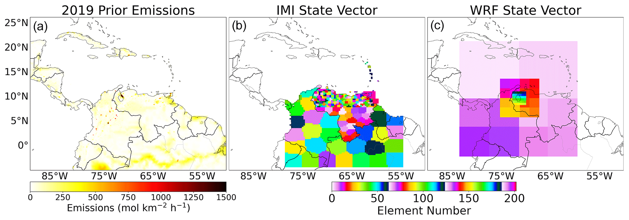
Figure 1 Prior emissions used in the inversion (a) and state vector elements used in the IMI (b) and WRF (c) inverse analyses. The different WRF domains can be discerned based on the resolution of the state vector elements, where the outer domains were set up to obtain an accurate representation of the background in the center domain.

2.2 National model: Integrated Methane Inversion

We use the Integrated Methane Inversion (IMI; Varon et al., 2022), which provides an analytical inversion framework using the Goddard Earth Observing System – Chemistry (GEOS-Chem 13.4.0) as its transport model (http://geos-chem.org, last access: 1 August 2022). The GEOS-Chem forward model runs are simulated on a 0.25° × 0.3125° grid encompassing all of Venezuela, driven by GEOS Fast Processing (GEOS-FP) meteorological data from the NASA Global Modeling and Assimilation Office (Molod et al., 2012). We use the standard v2023-04 3 h IMI boundary and initial conditions based on monthly 10° smoothing of TROPOMI values over land and based on latitudinal averages over water (Shen et al., 2021; Varon et al., 2022) but optimize these in the inversion. Methane has a long atmospheric lifetime compared to its residence time in our IMI simulation, but nevertheless, the IMI includes sinks of methane from oxidation by OH and Cl (based on archived concentration fields from a full-chemistry simulation), stratospheric loss (Maasakkers et al., 2019), and soil uptake (Murguia-Flores et al., 2018). We run the IMI forward model for 2019 over the domain shown in Fig. 1b (4.3° S–17.5° N, 78.4–54.7° W, encompassing Venezuela), using December 2018 as a spinup to initialize the model's concentration field. We adapt the IMI framework to use the TROPOMI Science Product with our custom filtering (Sect. 2.1) and with our ensemble inversion approach including log-normal error distributions (Sect. 2.4).

2.3 Local model: Weather Research and Forecasting model with chemistry

To analyze emissions around Lake Maracaibo at a higher resolution, we use the Weather Research and Forecasting with chemistry (WRF-Chem) model version 4.1 (Powers et al., 2017; Skamarock et al., 2019). Because of the short residence time of methane in the domain compared to the atmospheric lifetime, we use a passive tracer model for our simulations. We perform simulations for 2018, 2019, and 2020, using December of the prior year as a spinup. As shown in Fig. 1c, the simulations were performed using three nested domains with 27, 9, and 3 km resolutions as they move in towards the Lake Maracaibo region. The outer two domains consist of 99 × 99 grid cells and the innermost domain has a 105 × 105 grid. These outer domains are set up to allow for an adequate representation of the background in the innermost domain. There are 33 vertical layers. The meteorology is driven by National Centre for Environmental Prediction (NCEP) data (National Centre for Environmental Prediction et al., 2000) with the “tropical” physics suite. We use the Copernicus Atmosphere Monitoring Service (CAMS) global forecast at 0.4° × 0.4° and a 6 h resolution to provide initial and boundary conditions on methane concentrations (Koffi and Bergamaschi, 2018), which we also optimize in the inversion. We use the soil sink from the IMI, but the effect is small (0.02 Tg a⁻¹).

2.4 Inverse methodology

We estimate both national and local emissions using Bayesian analytical inversion (Jacob et al., 2016) where we find the optimal posterior solution ($\widehat{\mathit{x}}$) for the state vector (x) as

$$\begin{array}{}\text{(1)}& \widehat{\mathit{x}}={\mathit{x}}_{\mathrm{A}}+{\mathbf{S}}_{\mathrm{A}}{\mathbf{K}}^{\mathrm{T}}{\left({\mathbf{KS}}_{\mathrm{A}}{\mathbf{K}}^{\mathrm{T}}+{\displaystyle \frac{{\mathbf{S}}_{\mathrm{O}}}{\mathit{\gamma }}}\right)}^{-\mathrm{1}}\left(y-\mathbf{K}{\mathit{x}}_{\mathrm{A}}\right),\end{array}$$

where x_A gives the prior state vector, S_A is the prior error covariance matrix, K is the Jacobian matrix representing the forward model, S_O is the observational error covariance matrix, γ is a regularization factor to prevent overfitting, and y is the observations. The posterior emissions can be evaluated using the posterior error covariance matrix $\widehat{\mathbf{S}}$ (Eq. 2) and averaging kernel A (Eq. 3, where I is the identity matrix) that quantifies the extent to which the posterior emissions are informed by the observations.

$$\begin{array}{}\text{(2)}& {\displaystyle }\widehat{\mathbf{S}}={\left(\mathit{\gamma }{\mathbf{K}}^{\mathrm{T}}{\mathbf{S}}_{\mathrm{O}}^{-\mathrm{1}}\mathbf{K}+{\mathbf{S}}_{\mathrm{A}}^{-\mathrm{1}}\right)}^{-\mathrm{1}}\text{(3)}& {\displaystyle }\mathbf{A}=\mathbf{I}-\widehat{\mathbf{S}}{\mathbf{S}}_{\mathrm{A}}^{-\mathrm{1}}\end{array}$$

For the national analysis, we use perturbation sensitivity simulations with the IMI (sampled using TROPOMI averaging kernels) to construct K and estimate the impact of emissions on the concentrations observed by TROPOMI, including offshore emissions. As TROPOMI does not provide enough information to individually optimize emissions from every grid cell, and running the associated sensitivity simulations for every grid cell would be computationally infeasible, we construct the state vector by grouping grid cells together using k-means clustering. Since most emissions are located in the northern half of Venezuela (Fig. 1a), we use the highest density of clusters (124) there. We use an additional 24 elements for the southern part of the country and another 50 in a 5° buffer zone around the country. The buffer zone elements mainly serve to correct the background concentrations of air floating into Venezuela. These include, for example, the wetland, coal, and oil emissions in neighboring Colombia that can be seen in Fig. 1a. We add three elements to optimize offshore emissions in Lake Maracaibo and off the northeastern coast of Venezuela. We also incorporate a state vector element to capture the sensitivity to the background by scaling the boundary conditions, giving 202 state vector elements in total (or 213 when scaling the boundary conditions monthly).

For the three annual WRF inversions, we simulate individual tracers for each state vector element (different parts of the domain) to include them in the state vectors. We divide the inner domain into a 6 × 6 grid (∼ 50 km × 50 km) to have a high resolution over the area of interest. We divide the outer and middle domains into 8 × 8 grids excluding the parts covered by the inner domain(s) and aggregate elements in the northwestern and northeastern corners of the outer domain, which are mostly covered by water. We use the state vector elements in the outer domains as buffer elements similar to the process used in the IMI. Finally, our 74-member state vector is completed with 12 elements scaling the monthly CAMS-based background. We also perform an inversion where we combine these last 12 elements into one annual background correction.

Table 1 Prior and posterior emissions for Venezuela and Lake Maracaibo in 2019 based on the IMI and WRF inversions of TROPOMI data in Tg a⁻¹.

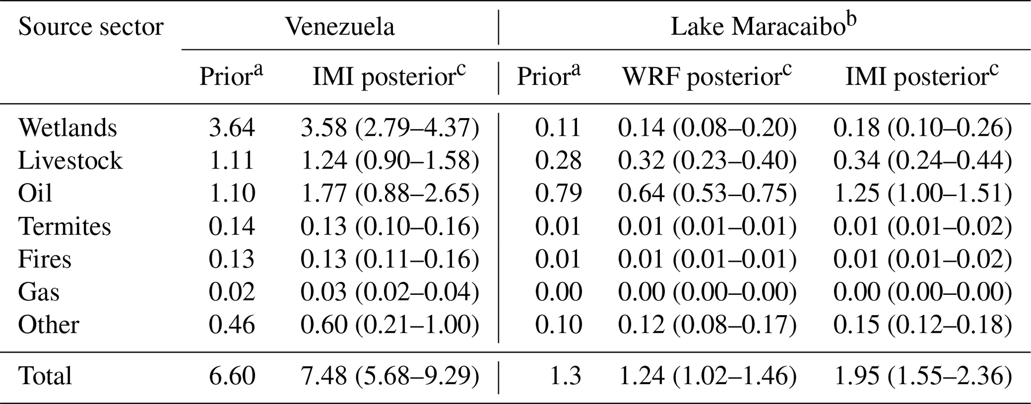
^a Prior emissions include 2019 oil, gas, and coal emissions from GFEI v2 (Scarpelli et al., 2022); 2018 livestock and other anthropogenic emissions from EDGAR v6 (Monforti Ferrario et al., 2021); wetland emissions from WetCHARTs v1.2.1 (Bloom et al., 2017); IMI-standard emissions from termites and geological seeps (Varon et al., 2022); and GFED v4 fire emissions (Randerson et al., 2018).
^b The Lake Maracaibo area encompasses 8.3–11.1° N, 72.7–69.9° W.
^c We report ensemble means and standard deviations.

Our prior bottom-up emissions are shown in Fig. 1a. We use 2019 oil, gas, and coal emissions from the Global Fuel Exploitation Inventory v2 (GFEI; Scarpelli et al., 2022) for all years. The remaining anthropogenic emissions, most prominently including livestock and waste management, are the 2018 emissions from the Emissions Database for Global Atmospheric Research v6 (EDGAR; Monforti Ferrario et al., 2021). The recent EDGAR v7 inventory (Crippa et al., 2022; European Commission and Joint Research Centre et al., 2021) estimates that Venezuelan livestock and waste management emissions changed by less than 5 % between 2018 and 2020. Natural emissions from wetlands come from WetCHARTs v1.2.1 (Bloom et al., 2017), and we included IMI-standard emissions from termites and geological seeps (Varon et al., 2022) as well as fire emissions from the Global Fire Emissions Database v4 (GFED; Randerson et al., 2018). Total emissions and maps for individual source sectors are included in Table 1 and in Fig. A1.

When comparing the model to TROPOMI for the inversion, we aggregate observations on a 0.2° grid to reduce the influence of small-scale transport errors (Maasakkers et al., 2022). We use an observational error of 15–19 ppb based on the standard deviation of the prior model–observation mismatch. To analyze the sensitivity of our inversions and estimate their uncertainties, we construct an ensemble of inversions, varying inputs (e.g., scaling prior emissions), assumptions (e.g., varying the error distribution), and settings (e.g., varying the regularization). To generate our ensemble, we (1) use prior emissions with a uniform scaling of 70 %, 100 %, and 130 % of prior emissions; (2) use observations over just the Lake Maracaibo area or over the entire (IMI or WRF) model domain; (3) aggregate observations over resolutions of 0.1, 0.2, and 0.5°; (4) find an optimal regularization factor of γ=0.25 based on L-curve analysis (Hansen, 2000) and include inversions with γ=0.1 and γ=0.5 as well; (5) use normal or log-normal errors following Maasakkers et al. (2019); (6) use the TROPOMI filters with the filtering described in Sect. 2.1 or Qa=1 filtering; (7) optimize the boundary conditions on a monthly or annual basis; (8) use the TROPOMI data with and without the standard albedo correction; and (9) assume that errors in aggregated observations scale with the central limit theorem ($\sim \sqrt{n}$) or do not decrease, when aggregating n observations. We report the means and conservative uncertainty ranges based on standard deviations of the resulting 1728-member ensembles for the IMI and WRF analyses.

2.5 Supporting satellite data

We use data from three satellite instruments to provide context for the TROPOMI-based results. The SCIAMACHY instrument aboard the ENVIronmental SATellite (ENVISAT) was the first satellite instrument to provide global coverage of total column methane data (Frankenberg et al., 2005, 2006). Operational between 2003 and 2012, it had a resolution of 30 km × 60 km. Observations after 2005 are of lower quality because of detector degradation (Kleipool et al., 2007). SCIAMACHY uses the 1.65 µm absorption band of methane, which allows the use of co-retrieved CO₂ in the proxy method. In that method, the observed ratio of methane to CO₂ is multiplied by a prior (modeled) CO₂ column to estimate total column methane, making the retrieval less sensitive to artifacts and atmospheric scattering. We use the proxy retrieval data of Frankenberg et al. (2011).

GOSAT was launched in 2009 and observes methane total column mixing ratios using its Thermal and Near infrared Sensor for carbon Observation – Fourier Transform Spectrometer (TANSO-FTS) instrument (Butz et al., 2011; Schepers et al., 2012; Kuze et al., 2016). In its default mode, GOSAT observes circular pixels of 10.5 km in diameter, separated by ∼ 250 km, at 13:00 LT. The observation track is repeated every 3 d, while a target mode can be used to observe additional locations. Like SCIAMACHY, GOSAT uses the 1.65 µm absorption band that is used in both full-physics and proxy retrievals. We use the University of Leicester v9.0 proxy product (Parker and Boesch, 2020). Data from its successor, GOSAT-2, are available starting in February 2019 (Suto et al., 2021). We use GOSAT-1 here to have uniform data across the studied time period.

The Suomi National Polar-Orbiting Partnership (SNPP) and NOAA-20 (J01) satellites both carry a VIIRS (Visible Infrared Imaging Radiometer Suite) multispectral imager that can be used to detect radiant emissions from gas flares in the 1.6 µm band at a 750 m spatial resolution (Elvidge et al., 2013). These observed heat radiances can be converted to flared gas volumes using the Stefan–Boltzmann law and a calibration based on reported volumes of flared gas (Elvidge et al., 2016). This approach has been calibrated and used at both the field level and the well level (Zhang et al., 2020; Maasakkers et al., 2022). Here we use the NightFire v3.0 product (Elvidge et al., 2013) together with the well-level calibration from Maasakkers et al. (2022), who assume a methane content of 95 %, to estimate the amount of gas/methane flared at sites in the Lake Maracaibo region.

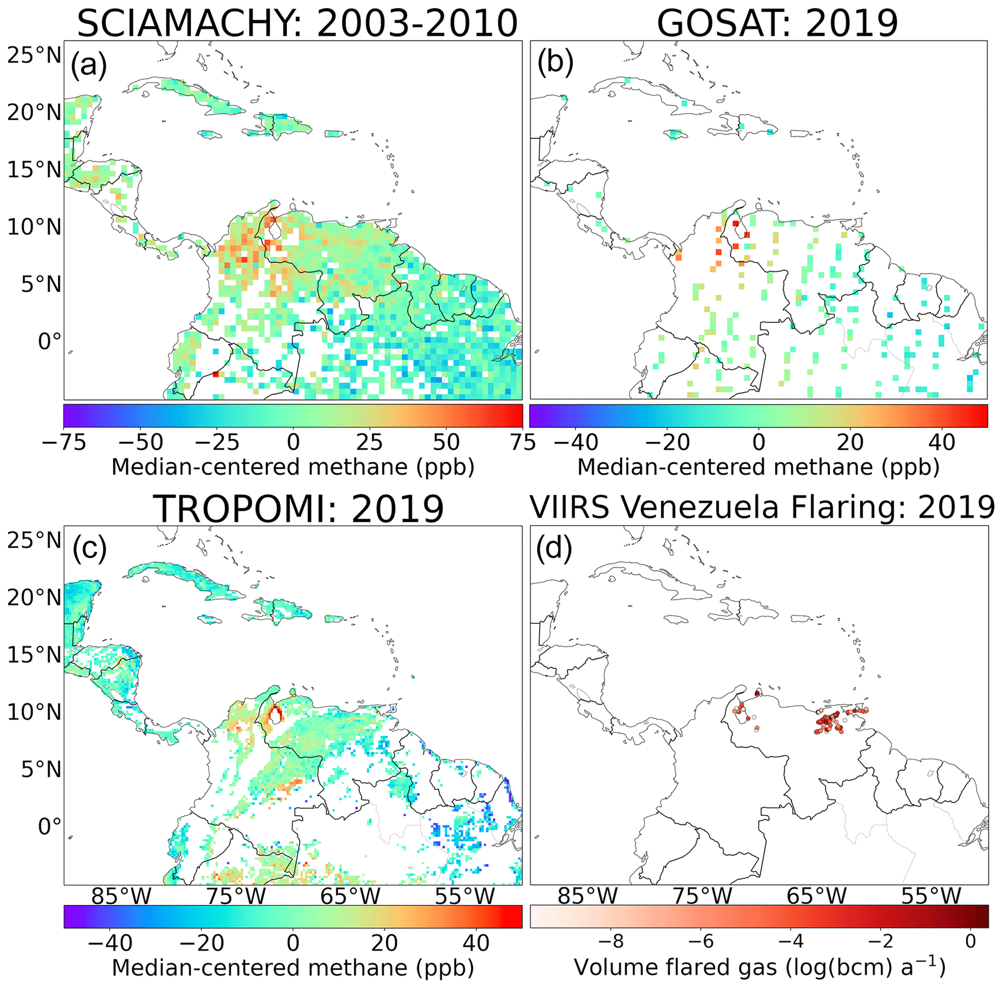
Figure 2 Average methane enhancements over northern South America from SCIAMACHY in 2003–2010 (a), GOSAT in 2019 (b), and TROPOMI in 2019 (c). The median values of the individual images have been subtracted to obtain median-centered enhancements. SCIAMACHY and GOSAT are visualized on a 0.5° grid, while TROPOMI is shown on a 0.2° grid. Only grid cells with at least five observations are shown. All panels have some saturated values. Panel (d) shows the facility-level amounts of gas flared based on radiant heat observed by VIIRS in 2019 in billion cubic meters of natural gas (bcm).

3 Results and discussion

Figure 2 compares the coverage of SCIAMACHY in 2003–2010 (Fig. 2a) with that of TROPOMI (Fig. 2b) and GOSAT (Fig. 2c) in 2019. The figure shows the vast improvement provided by TROPOMI compared to SCIAMACHY in terms of precision (where even the multi-year average contains very noisy observations) and in terms of coverage compared to GOSAT. Some areas lack TROPOMI coverage because of steep elevation gradients, such as in the Andes, or prohibitively low albedo values, such as over the Amazon. Total column values are lower over areas with higher elevations where the low-concentration stratosphere has a larger relative impact on the column-averaged values. Some areas (eastern Colombia, the Amazon) show some albedo-induced high and low methane values that are based on only a few observations. Enhanced methane values are seen around Lake Maracaibo in western Venezuela using all instruments, with the eastern coast of the lake in particular standing out in TROPOMI. In annual GOSAT data (Fig. A2), persistent enhancements can be seen around the lake between 2010 and 2020, but the limited spatial coverage makes it hard to attribute these enhancements to underlying emissions. About 20 d of TROPOMI data in 2019 has been manually identified as having plume-like signals originating from the lake area, even though the combination of persistent cloud cover, proximity to water, and complicated topography makes seeing fully developed plumes impossible. Figure 2d shows Venezuelan facility-level flared gas volumes estimated based on 2019 VIIRS data. Clusters of flares can be seen both on and along Lake Maracaibo as well as in the Orinoco basin in the eastern part of the country, matching the distribution of oil production emissions (Fig. A1).

Figure 3 Inversion results from the 2019 IMI inversion over Venezuela with (a) posterior : prior scaling factors; (b) posterior emissions; (c) averaging kernel sensitivities; and (d) nationally aggregated prior and posterior emissions per source sector, with the fraction of emissions constrained by averaging kernels (A) above 0.05 shown in green. Values shown are means of the inversion ensemble, with the ranges showing the associated ensemble standard deviations.

Compared to TROPOMI, our 2019 IMI-based inversion improves our simulation's mean absolute bias from 15 to 12 ppb and increases the correlation between model and observations from r=0.47 to 0.53 (Fig. A1a and b). We find an annual average correction of the background, represented by the IMI boundary and initial conditions, of 0.3 %. Figure 3 shows the results for the 2019 IMI-based inversion over Venezuela. The prior estimate for Venezuela totals 6.6 Tg a⁻¹, and the ensemble-mean posterior estimate is 7.5 Tg a⁻¹ with an ensemble standard deviation of 1.8 Tg a⁻¹. Figure 3a and b show that emissions are scaled up over areas with the most emissions: Lake Maracaibo in the northwest and the Orinoco Belt in the northeast. Global studies interpreting satellite data with GEOS-Chem as the transport model also found upward corrections, albeit using the higher Scarpelli et al. (2020) emissions as prior emissions (Qu et al., 2021; Lu et al., 2021). Emissions in most of the low-emitting southern part of the country are scaled down slightly. However, the diagonal of the averaging kernel (Fig. 3c) shows that there is little information in the TROPOMI data for most of Venezuela, with the exception of the Lake Maracaibo emission hot spot. Many of the highest averaging kernel values fall in the buffer cells outside Venezuela, and the upward correction in the Orinoco basin is especially poorly informed by the satellite data. To estimate sector-specific posterior emissions (Fig. 3d and Table 1), we multiply the scale factors of each state vector element by their prior sectoral emissions. The three major sources of methane in Venezuela are oil production, wetlands, and livestock. We find the largest relative correction for oil, 1.6 (0.8–2.4), in large part driven by the upward correction over Lake Maracaibo. Oil production is responsible for 24 % (17 %–30 %) of national emissions, up from 17 % in the prior correction. Emissions from natural gas, fires, termites, and other sources all play very minor roles in both the prior and posterior emission totals. Also shown in Fig. 3d are the fractions of the emissions with some constraint from TROPOMI (an associated diagonal averaging kernel larger than 0.05, following Nesser et al., 2024). We find that for both oil and wetland emissions, a large fraction of emissions at the national level can not be constrained by the TROPOMI data (quantification of average wetland emissions is further complicated by the fact that we only have observations on clear-sky days). The associated spread of the inversion ensemble is mainly driven by the ensemble members that scale the prior emissions, as well as the number of observations used (for example, due to the data filtering), and the weight attributed to them in the inversion with the regularization factor, with some contribution from the albedo correction (Fig. A3). Overall, this indicates that at the current stage, evaluating national total emissions from Venezuela with a single year of TROPOMI data is not feasible with meaningful uncertainty.

Figure 4 Inversion results from the 2019 WRF inversion over Lake Maracaibo with (a) posterior : prior scaling factors; (b) posterior emissions; (c) averaging kernel sensitivities; and (d) aggregated prior and posterior emissions per source sector, with the fraction of emissions constrained by averaging kernels (A) above 0.05 shown in green. Values shown are means of the inversion ensemble, with the ranges showing the associated ensemble standard deviations.

Compared to TROPOMI, our 2019 WRF-based inversion improves the mean absolute bias over the Lake Maracaibo area from 57 to 12 ppb and increases the correlation between model and observations from r=0.42 to 0.47 (Fig. A4c and d). In the absence of suborbital observations, we use the proxy-method GOSAT (Fig. 2b) data as the most independent data set to evaluate our inversion results. We find that the mean absolute bias with GOSAT decreases from 71 to 19 ppb, mostly due to the upward correction to the CAMS background of 3 % on average, with some remaining bias due to a mean offset between GOSAT and TROPOMI over the region. We find that correlation between the model and GOSAT improves from r=0.56 to r=0.58, mainly due to corrections to emissions. Figure 4 shows the results of the WRF-based inversion over Lake Maracaibo, focusing on the results from the inner domain. Lake Maracaibo emissions are estimated at 1.2 (1.0–1.5) Tg a⁻¹ (Fig. A5); are dominated by oil production, 51 % (44 %–58 %) of total emissions; and are lower than the results based on the IMI inversion, 2.0 (1.6–2.4) Tg a⁻¹. The difference is mainly related to the oil estimates from the two inversions (source sector emission totals are included in Table 1). The averaging kernel sensitivities (Fig. 4c) show that the area east of Lake Maracaibo is the only area where TROPOMI provides significant information. This is not unexpected as the large prior emissions there would have a large effect on the scarce TROPOMI observations over the area. This is also the main area where emissions are decreased with respect to the prior ones, with most of the remainder of the domain showing a slight increase but very small averaging kernels. As Fig. 4d shows, the oil emissions are well characterized by the inversion as they are clustered in the area where TROPOMI provides most information, with an uncertainty range including the prior value. While inefficient flaring can play a role, we find oil emissions that are larger than the annual mass of methane flared in the area (0.6 Tg in 2019, assuming a 95 % methane content) based on VIIRS, suggesting that the majority of emissions come from other sources such as leaks or vents. Emissions from the other source sectors (predominantly livestock and wetlands) show small increases that are insignificant compared to the prior emissions and show relatively worse constraints than TROPOMI as a larger fraction of the emissions occurs outside of the well-constrained hot spot area.

To take advantage of the two independent model simulations and better understand the differences compared to the IMI inversion, we perform an additional WRF inversion (not included in the ensemble). Here, we resample the WRF simulation output to the IMI grid to perform a “most IMI-like” inversion and find Lake Maracaibo emissions of 1.4 Tg a⁻¹ compared to 2.3 Tg a⁻¹ when using equivalent inversion settings in the IMI framework. This resampling reduces the probability of plumes in WRF having large spatial mismatches with plumes seen in TROPOMI, which could lead to underestimation of the emissions. The remaining difference after aligning sampling suggests that the underlying transport is the main culprit. There are other differences between the models, such as the representation of the background, loss processes, and the stratosphere, but these are unlikely to have a major effect on the emission estimate for the concentrated hot spot area because of the damping influence of the optimizations of the background and buffer elements around the area. To further investigate the differences in transport, we compare the WRF output 10 m wind speed based on NCEP boundary and initial conditions to the GEOS-FP 10 m wind (used in the IMI) over the lake (sampled at 9.8° N, 71.5° W). We find that at the overpass of TROPOMI (∼ 18:00 UTC), the GEOS-FP average wind speed in 2019 is 2.8 ± 1.2 m s⁻¹ (standard deviation), a factor of 1.9 larger than the WRF-derived wind of 1.5 ± 0.8 m s⁻¹. The independent ERA5 reanalysis (Hersbach et al., 2020) gives a wind speed of 1.9 ± 0.7 m s⁻¹ for the same time and location. Similarly, we find that winds between 975 and 800 hPa in GEOS-FP are a factor of 1.6 larger than in NCEP, which is used to drive the WRF boundary conditions. The lower WRF winds lead to a slower ventilation of the area and result in a buildup of methane. Therefore, the WRF inversion “requires” lower emissions to explain the same methane enhancement in TROPOMI than the IMI inversion, which has a stronger wind speed in the area, showing the importance of reliable meteorological data. While the lower wind speeds calculated by WRF may partly result from the higher resolution of the model as it attempts to resolve around the local terrain, the large difference in the data driving the boundaries is considered to be the most likely culprit. As there are no observations or large emissions nearby (partly due to the proximity to the ocean), the transport-induced difference in emissions is not compensated for by nearby grid cells but instead carries through to the local budget.

Figure 5 shows annual 2018–2020 local emissions for the Lake Maracaibo region based on annual WRF inversions. Compared to GOSAT, the mean bias over these 3 years improves from 73 to 23 ppb, while correlation improves from r=0.49 to r=0.53. As the uncertainty ranges from the inversion ensemble overlap, a significant trend cannot be seen, but both the temporal evolution of the base inversion and that of the other ensemble members suggest a decrease. This decrease would be consistent with the (also shown) 2018–2020 decreases in flaring activity observed by the VIIRS satellite instruments (∼ 20 % drop), with reported marketed oil production (∼ 60 % drop; Rystad Ucube, 2022), and with reported marketed gas production (∼ 90 % drop, albeit absolute numbers are small; Rystad Ucube, 2022). Our decrease is close to the 30 % decrease in 2018–2020 Venezuelan oil/gas emissions predicted by EDGAR v7. Even including the 2018–2020 drop in the base WRF inversion (∼ 20 %), our results suggest increasing methane intensity because of the strongly reduced production. Following Schneising et al. (2020), we express the emissions as methane emission intensity compared to the energy content of the combined oil and gas production in the area. We find intensities of 11 %, 13 %, and 23 % for 2018–2020, with a value of 21 % for 2019 based on the IMI analysis. These values are much higher than the intensities of 1 %–4 % Schneising et al. (2020) found for production regions in the United States and in Turkmenistan. The increasing methane emission intensity trend points at emissions that are independent of the amount of oil and gas production and are likely related to the neglected or abandoned infrastructure in the region.

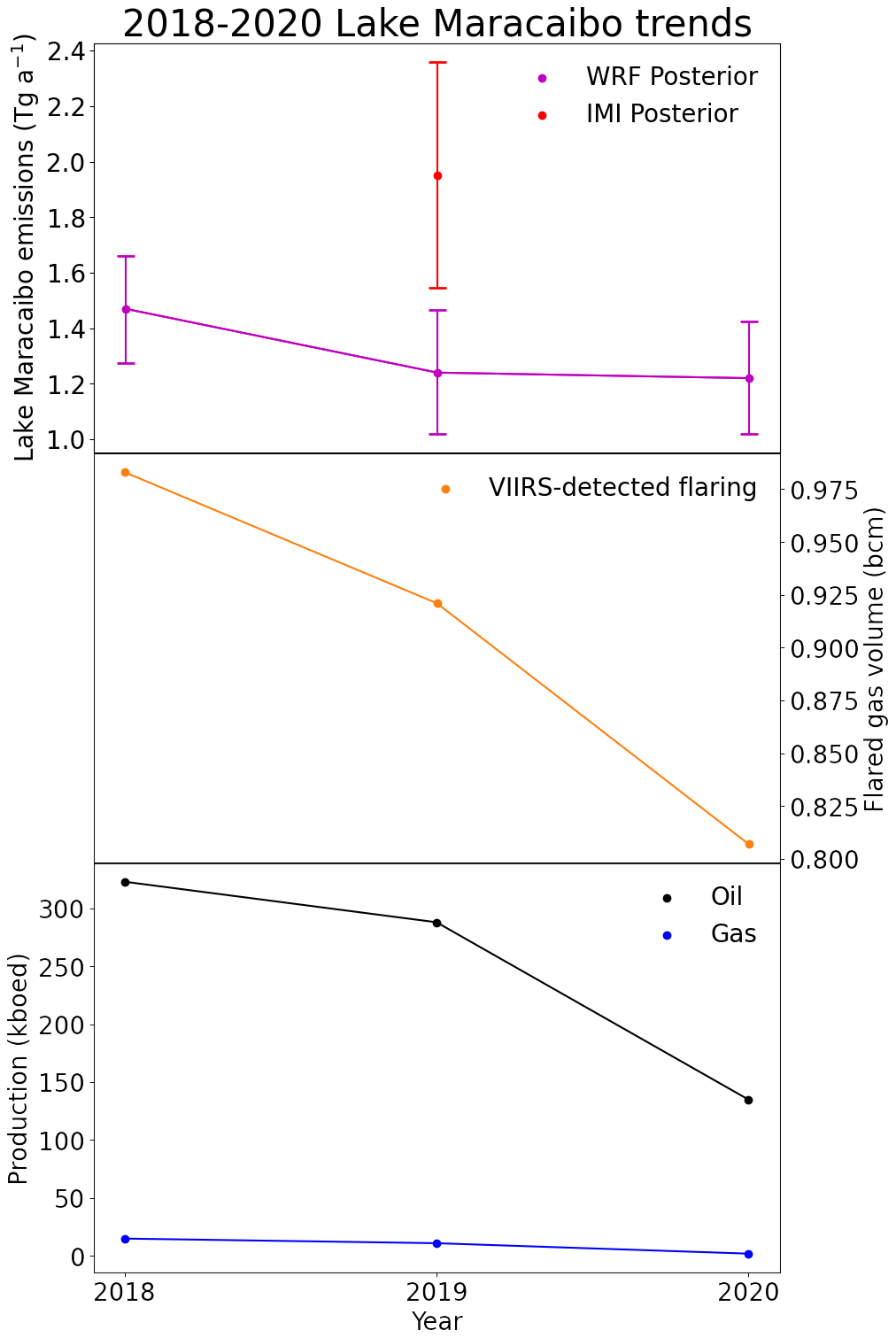
Figure 5 Annual results from the 2018–2020 inversions, suggesting a downward trend in emissions over the region. Also shown are VIIRS-observed flared volumes of natural gas and reported oil and gas production for the same domain (Rystad Ucube, 2022), all showing decreases from 2018 to 2020.

4 Conclusions

We performed analytical inversions with 2018–2020 TROPOMI satellite methane data using two different models to estimate methane emissions over Venezuela, with a focus on emissions from the oil production area around Lake Maracaibo that has long been identified as a methane hot spot. TROPOMI provides unprecedented daily global coverage at a city-scale resolution, showing a clear hot spot around the eastern shore of the lake, but the area remains difficult to observe due to elevation, low surface albedo, and persistent cloud cover.

Our national analysis using the IMI framework shows 2019 emissions are a factor of 1.1 (0.9–1.4) higher than predicted by bottom-up inventories, with emissions from oil production showing the largest relative correction of a factor of 1.6 (0.8–2.4). TROPOMI can provide limited information on Venezuelan emissions because the number of observations in the area is limited by elevation gradients, persistent cloud cover, and low surface albedo. Based on the averaging kernel of the (TROPOMI) inversion, the satellite data cannot constrain about half of the posterior national emissions of 7.5 (5.7–9.3) Tg a⁻¹. Emissions over the eastern Orinoco production basin in particular show little TROPOMI sensitivity. While the inversion provides only limited information on wetland emissions, it does show sensitivity to the Lake Maracaibo area.

Our focused analysis of the Lake Maracaibo region using WRF shows that the 2019 emissions in the area of 1.2 (1.0–1.5) Tg a⁻¹, predominantly from oil production, are well constrained by TROPOMI and are consistent with bottom-up inventories but are lower than the local IMI results. We find that the difference from the IMI is due to the stronger winds in the GEOS-FP meteorology driving the IMI compared to the NCEP winds used in the initial and boundary conditions of WRF. Analyzing the 2018–2020 annual emissions over Lake Maracaibo, we find a decrease in emissions of ∼ 20 % that is within the uncertainty margin of our ensemble, that together with strongly decreased local oil/gas production leads to more than doubling of the implied methane emission intensity (11 % to 23 %) expressed against combined oil and gas production, much higher than previous studies have found for other oil/gas production regions around the globe. Our work provides better insight into Venezuelan emissions but also improves our understanding of the capabilities of using satellite data and (inverse) models at different scales. Our work can be used to target future analysis, including extending our analysis for later years and incorporating facility-scale methane observations from high-spatial-resolution satellites and suborbital observations (including of methane isotopes) to give additional insight into the (evolution of) local emissions from different source sectors and serve as an independent verification of satellite-based inversion results.

Appendix A: Supplemental figures

Figure A1 Prior emissions by source sector in 2019, as described in Table 1.

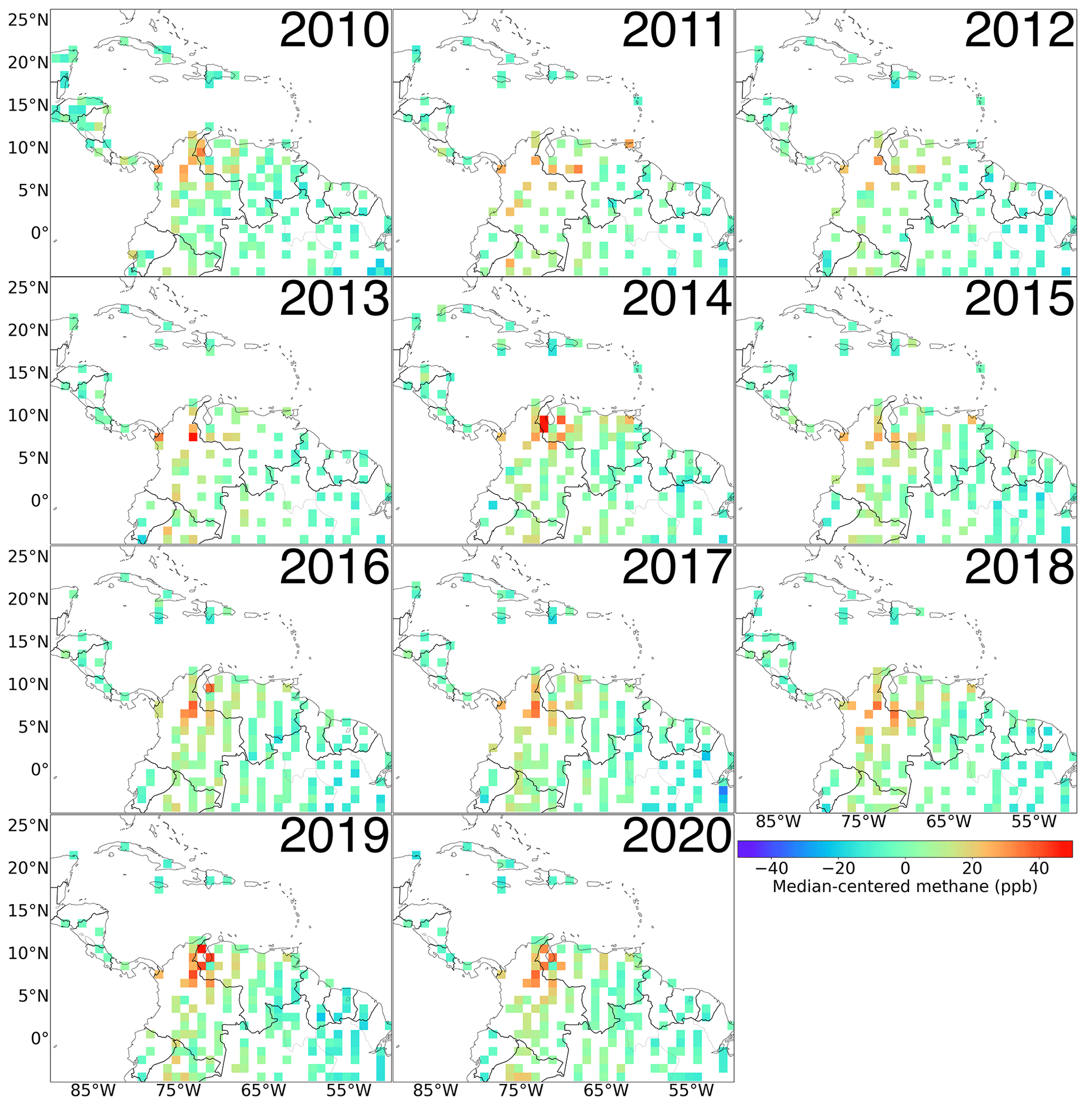
Figure A2 Annual average methane enhancements over northern South America from GOSAT for 2010–2020 on a 0.5° grid. The median values of the individual images have been subtracted to obtain median-centered enhancements. Only grid cells with at least five observations are shown. All panels have some saturated values.

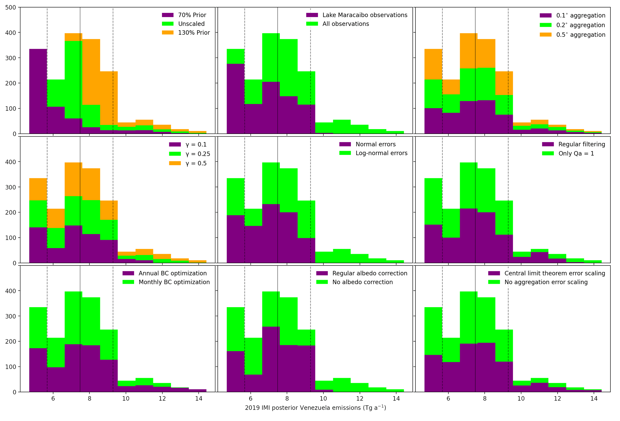
Figure A3 Histograms showing total Venezuelan emissions from the IMI inversion ensemble for 2019. Individual panels show the effect of the different ensemble characteristics described in Sect. 2.4. The solid line shows the ensemble mean (7.48 Tg a⁻¹), and the dashed lines show the associated standard deviations (± 1.81 Tg a⁻¹).

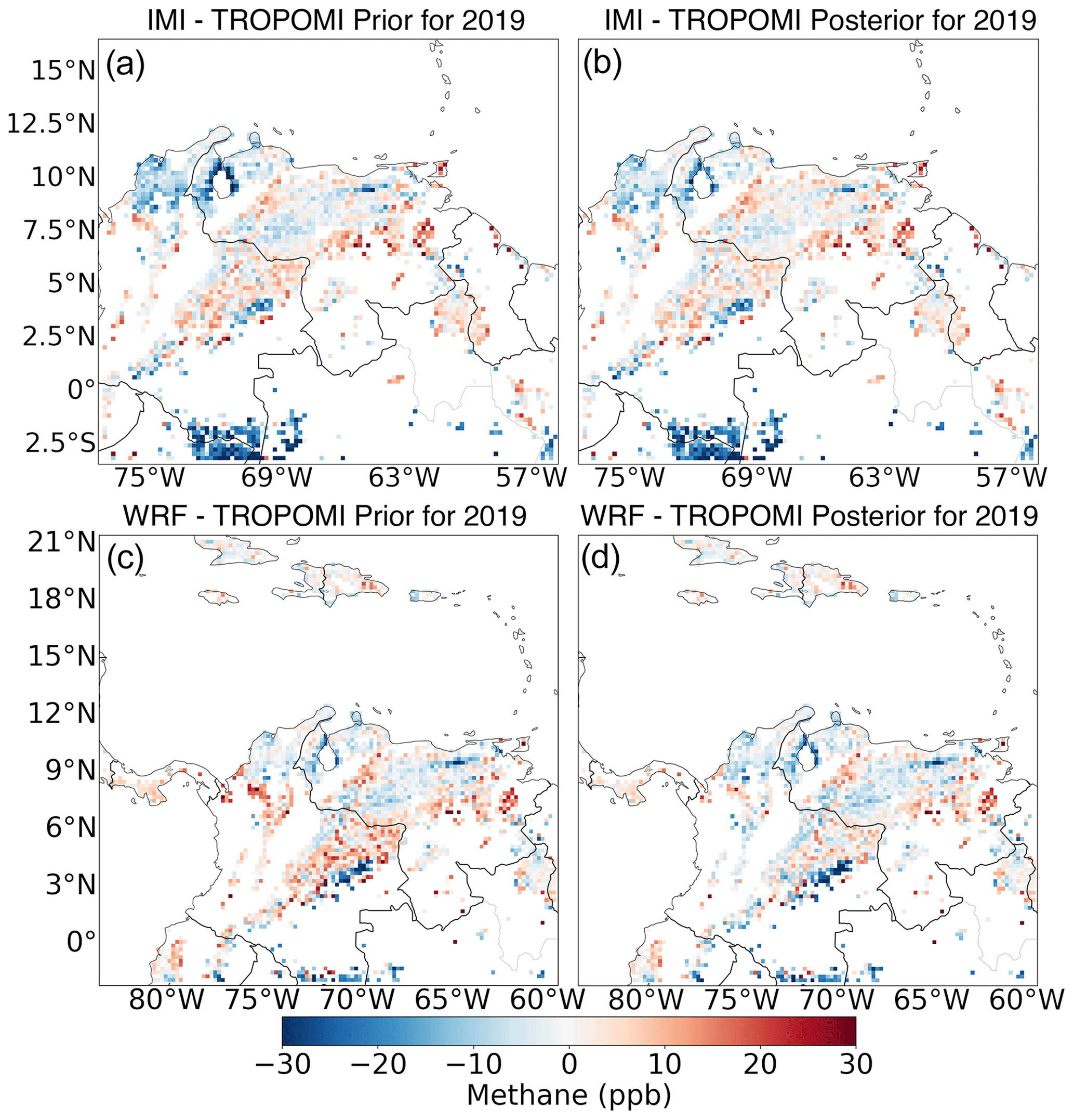
Figure A4 Differences in 2019 between TROPOMI and the IMI (a, b) and the WRF (c, d) prior and posterior simulations. Only grid cells with at least five observations are shown. Prior panels already include the corrections to the background from the inversions to isolate the influence of corrections on emissions. Changes between the prior and posterior simulations are small visually as averages only depend on a few (sometimes uncertain) observations, not all differences are attributable to emissions, and the state vectors have a very limited resolution over much of the domain. The clearest differences can be seen at the northern edge of Lake Maracaibo. The inversions cover slightly different domains, as shown in Fig. 1.

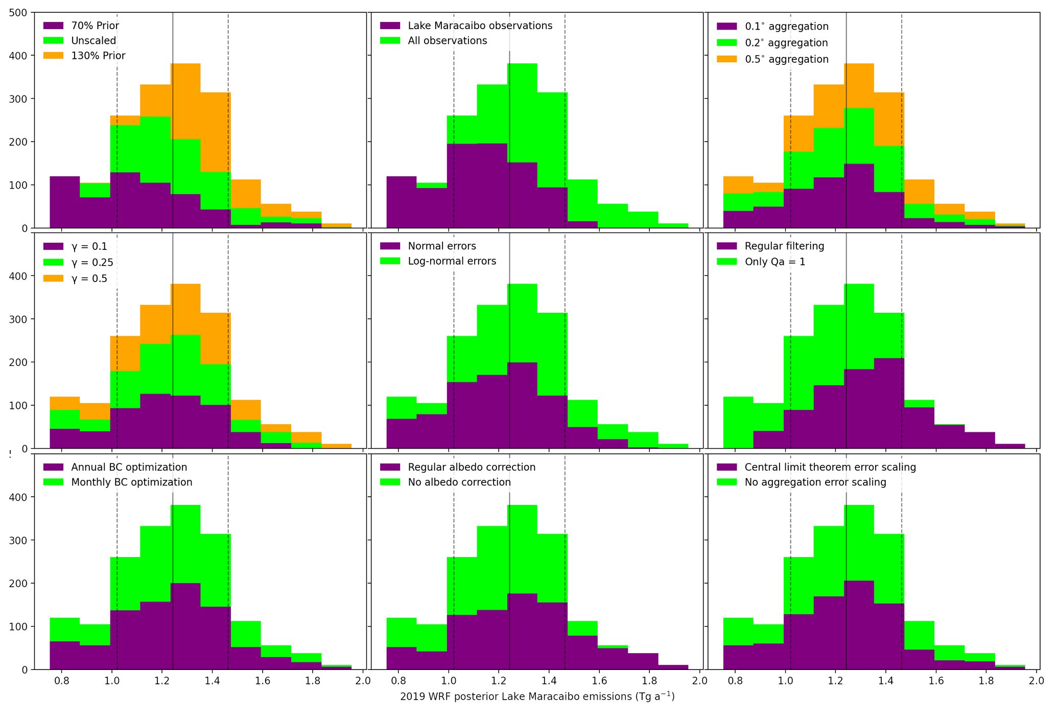
Figure A5 Histograms showing Lake Maracaibo emissions from the WRF inversion ensemble for 2019. Individual panels show the effect of the different ensemble characteristics described in Sect. 2.4. The solid line shows the ensemble mean (1.24 Tg a⁻¹), and the dashed lines show the associated standard deviations (± 0.22 Tg a⁻¹).