Effects of radiative cooling on advection fog over the northwest Pacific Ocean: observations and large-eddy simulations

During boreal summer, prevailing southerlies traverse the sharp sea surface temperature (SST) front in the northwest Pacific (NWP) Ocean, creating a stable air–sea interface characterized by surface air temperature (SAT) higher than SST, which promotes the frequent occurrence of advection fog. However, long-term shipborne observations reveal that during episodes of advection fog, SAT usually decreases below SST, with a peak relative frequency (∼ 34.5 %) in all fog observations before sunrise and a minimum relative frequency (∼ 18.8 %) before sunset. From a Lagrangian perspective, this study employs a turbulence-closure large-eddy simulation (LES) model to trace a fog column across the SST front and investigates how SAT drops below SST during an advection fog event. The LES model, incorporating constant solar radiation, successfully simulates the evolution of advection fog and the negative difference between SAT and SST. Simulation results show that once the near-surface air condenses, thermal turbulence is generated by strong longwave radiation cooling (LWC) at the fog top. The influence of LWC on the fog layer surpasses the cooling effect of the near-surface mechanical turbulence ∼ 2 h after the fog formation while the fog column is still positioned over the SST front. When the fog column arrives at the cold flank of the SST front, the top-down-developing mixed layer induced by the LWC reaches the surface, causing SAT to drop below SST. The LES model with diurnal solar radiation successfully simulates the observational diurnal variation in SAT and SST (SAT-SST) during the fog event, suggesting that the model captures the essential processes responsible for negative SAT-SST. This study highlights the significance of fog-top cooling and its associated thermal turbulence in the evolution of advection fog. Given the challenges faced by numerical weather prediction models in forecasting sea fog, our findings suggest that observations of negative SAT-SST during advection fog episodes present an opportunity to enhance the performance of these models in simulating the thermal turbulence induced by the LWC at the fog top.

1 Introduction

The northwest Pacific Ocean experiences heavy sea fog during summer (Wang, 1985; Koračin and Dorman, 2017), which is of great importance due to its significant impact on maritime activities (Gultepe et al., 2007; Trémant, 1987). However, present numerical weather prediction models struggle to accurately forecast sea fog (Gao et al., 2007), partly because their coarse resolutions inadequately resolve boundary-layer processes within the thin fog layer with depths of hundreds of meters (Yang and Gao, 2020). Therefore, enhancing our understanding of turbulent boundary-layer processes becomes imperative for refining the accuracy of sea fog predictions.

The sea surface temperature (SST) gradient associated with the Kuroshio Extension often triggers advection fog during summertime warm advection (Wang, 1985; Koračin and Dorman, 2017). Prevailing southerlies on the western flank of the subtropical high transport warm, humid air across the Kuroshio Extension front (Zhang et al., 2014; Long et al., 2016; Koračin and Dorman, 2017), which cools the near-surface humid air through mechanical turbulence, leading to air saturation and fog formation (Taylor, 1917; Rodhe, 1962; Lewis et al., 2004; Gao et al., 2007; Yang and Gao, 2020). Nevertheless, near-surface cooling induced by mechanical turbulence appears to be crucial in the initial phase of advection fog (Hu et al., 2006).

Once fog forms, the longwave radiation cooling (LWC) effect at the fog top commences to influence fog evolution. Earlier observational studies conjectured that the LWC at the fog top plays an important role in the fog's development and maintenance (Douglas, 1930; Petterssen, 1938; Findlater et al., 1989). LWC at the fog top induces negative buoyancy and thermal turbulence (Bretherton and Wyant, 1997; Gerber et al., 2005, 2013; Guan et al., 1997; Yamaguchi and Randall, 2008; Koračin and Dorman, 2017). This thermal turbulence further promotes vertical mixing and cools the fog layer (Rogers and Koračin, 1992; Koračin et al., 2001, 2005; L. Yang et al., 2018). Huang et al. (2015) identified a so-called thermal-turbulence interface, which separates thermal turbulence induced by the fog-top LWC and near-surface mechanical turbulence. Despite previous studies recognizing the significance of LWC at the fog top, its relative importance to near-surface cooling by mechanical turbulence remains to be determined.

Observational evidence underscores the significance of LWC at the fog top, as the surface air temperature (SAT) occasionally falls below SST during advection fog episodes. This means that the sea surface acts to heat the fog layer (referred to as sea fog with sea surface heating or SSH hereafter). Instances of SSH fog have been reported in advection fog events over the Yellow Sea (Zhang et al., 2012; Zhang and Ren, 2010), in the fog off the California coast (Leipper, 1948, 1994) and off the northeastern coast of Scotland (Findlater et al., 1989). Based on long-term buoy observations, L. Yang et al. (2018) found that the relative frequency of SSH fog in advection fog reaches up to ∼ 30 % over the Yellow Sea in summer. Their composite analysis revealed that SSH fog is associated with stronger atmospheric subsidence, a drier free atmosphere, and sharper capping inversions, indicative of a crucial role of the fog-top LWC for SSH fog. However, limited observations of the boundary-layer vertical structure over the sea inhibit the understanding of how fog-top LWC influences advection fog and leads to a negative SAT and SST (hereafter SAT-SST).

In comparison to numerical weather prediction models, large-eddy simulations (LESs) with higher resolutions are capable of explicitly resolving larger thermal-turbulence eddies within the boundary layer. LESs have been successfully employed in studies related to clouds (Bretherton and Wyant, 1997; Wyant et al., 1997; Savic-Jovci and Stevens, 2008; McGibbon and Bretherton, 2017) and continental fog (Nakanishi, 2000; Bergot, 2013, 2016; Maronga and Bosveld, 2017; Schwenkel and Maronga, 2019). Recently, the application of LESs has extended to sea fog (Yang et al., 2021; Wainwright and Richter, 2021). Yang et al. (2021) used the climatological subsidence to force a LES model to study an advection fog event over the northwest Pacific (NWP). They found that the fog-top thermal turbulence induced by the LWC entrains the drier free-atmospheric air into the boundary layer, which evaporates near-surface fog droplets, leading to a transition of fog into stratus. This simulated fog-to-stratus transition based on LESs is consistent with that in long-term observations. Wainwright and Richter (2021) attempted to use LESs to examine the sensitivity of sea fog to the cloud-droplet number concentration, turbulent mixing, and SAT-SST.

The present study primarily focuses on the SSH fog during advection fog episodes. We first analyze the statistical features of the SSH fog over the NWP using long-term shipborne observations. SSH fog was observed during the advection fog episode studied by Yang et al. (2021). Thus, this study extends the LES conducted by Yang et al. (2021) by forcing the LES with more realistic free-atmospheric subsidence to specifically investigate the boundary-layer processes responsible for SSH fog. We quantify the heat budgets of the fog layer based on the LES results to compare the effects of fog-top LWC and near-surface cooling and identify the interface between thermal and mechanical turbulence. The results highlight the importance of the fog-top cooling and its induced thermal turbulence on the evolution of advection fog.

The paper is organized as follows. Section 2 describes the data sets and methods used in this study. Section 3 analyzes the observational characteristics of sea fog with SSH over the NWP. Section 4 presents the simulation results obtained using constant solar radiation and diurnal-cycle radiation. Section 5 provides a summary and discussions.

2 Data and method

2.1 ICOADS and ERA5

We employ shipborne observations provided by the International Comprehensive Ocean-Atmosphere Data Set (ICOADS; Worley et al., 2005) to investigate the occurrence of sea fog over the summer NWP. Fog is identified when the present-weather code is between 10 and 12 or 40 and 49 and the visibility is lower than 1 km (Bari et al., 2016; Yang et al., 2021). Additionally, we also use SST, SAT, and 10 m winds to examine the sea–air interface conditions during sea fog. We include ∼ 6×10⁴ fog reports over the NWP between 1998 and 2018 to explore sea fog climatologies and select a fog case that took place during 1–4 July 2013 for further analysis and simulation.

To construct the idealized initial conditions for the sea fog simulation, we use the fifth generation of the European Centre for Medium-Range Weather Forecasts atmospheric reanalysis (ERA5; Hersbach et al., 2020). ERA5 fields are on a 0.25°×0.25° grid with 16 levels below 500 hPa.

2.2 UCLA-LES model

UCLA-LES is a three-dimensional, turbulence-closure boundary-layer model with prognostic variables such as the total water mixing ratio q_t, the liquid water potential temperature θ_l, and three components of wind. This model is often used to simulate stable, neutral, and convective boundary layers (Stevens et al., 2005).

The parameterization for subgrid fluxes in UCLA-LES is based on the Smagorinsky–Lilly model (Smagorinsky, 1963; Lilly, 1967) to satisfy the model closure. This model can explicitly compute thermal-turbulence flux and appropriately describe the turbulent mixing process within the boundary layer (Stevens et al., 2005; Jiang et al., 2006). Surface fluxes of momentum, temperature, and moisture are computed based on the similarity theory (Stevens, 2010). We set specific surface properties to represent oceanic conditions and prescribe surface temperature and specific humidity. Radiative transfer calculations are performed using the δ-four-stream method (Fu and Liou, 1993; Pincus and Stevens, 2009), and radiative fluxes are based on background profiles of pressure, temperature, humidity, and ozone content (Stevens et al., 2003). The model has a warm-rain microphysical scheme (Seifert and Beheng, 2001), assuming that cloud droplets are in equilibrium at a fixed concentration. The microphysics process accounts for the interactions within the same types and between different types of cloud and raindrops. We set a specified 100×10⁶ g kg⁻¹ cloud-droplet mixing ratio in our simulations. To capture the delicate radiative and turbulent processes, we set horizontal grid spacing as 20 m and the vertical grid spacing as 1 m below 50 m and 5 m above 50 m. The simulation domain is 1500 m × 1500 m × 2000 m.

2.3 Diagnostic equations

We analyze the budget of domain-averaged heat and water vapor to investigate the related physical processes responsible for sea fog evolution. The heat budget is calculated using

$$\begin{array}{}\text{(1)}& {\displaystyle \frac{\partial \stackrel{\mathrm{‾}}{\mathit{\theta }}}{\partial t}}=-{\displaystyle \frac{\partial \stackrel{\mathrm{‾}}{w{}^{\prime }\mathit{\theta }{}^{\prime }}}{\partial z}}-{\displaystyle \frac{L_{\mathrm{v}}E}{\stackrel{\mathrm{‾}}{\mathit{\rho }}{C}_{\mathrm{p}}}}-{\displaystyle \frac{\mathrm{1}}{\stackrel{\mathrm{‾}}{\mathit{\rho }}{C}_{\mathrm{p}}}}{\displaystyle \frac{\partial \stackrel{\mathrm{‾}}{Q}}{\partial z}},\end{array}$$

where θ is potential temperature. The term on the right-hand side (RHS) describes the heat change from turbulent mixing, latent heat releasing, and the radiation effect. $\stackrel{\mathrm{‾}}{w{}^{\prime }\mathit{\theta }{}^{\prime }}$ is the sum of the resolved and sub-scale parameterized turbulent heat flux. E is the amount of water vapor produced by liquid phase transition. L_v is the latent heat release of condensation or evaporation. ρ is air density. C_p=1004.67 J kg⁻¹ K⁻¹ is the specific heat of moist air. Q is radiation flux. The water vapor budget equation is

$$\begin{array}{}\text{(2)}& {\displaystyle \frac{\partial \stackrel{\mathrm{‾}}{q_{\mathrm{v}}}}{\partial t}}=-{\displaystyle \frac{\partial \stackrel{\mathrm{‾}}{w^{\prime }{q}_{\mathrm{v}}^{\prime }}}{\partial z}}+{\displaystyle \frac{E}{\stackrel{\mathrm{‾}}{\mathit{\rho }}}},\end{array}$$

where q_v is the water vapor mixing ratio. The terms on the RHS describe the q_v change from the turbulent mixing effect and evaporation/condensation. $\stackrel{\mathrm{‾}}{w^{\prime }{q}_{\mathrm{v}}^{\prime }}$ is the sum of the resolved and sub-scale turbulent water vapor flux.

To diagnose the turbulent mixing process responsible for heat and moisture variation, we compute the turbulent kinetic energy (TKE) budget using

$$\begin{array}{}\text{(3)}& {\displaystyle \frac{\partial \stackrel{\mathrm{‾}}{\mathrm{TKE}}}{\partial t}}=+{\displaystyle \frac{g}{\stackrel{\mathrm{‾}}{{\mathit{\theta }}_{\mathrm{v}}}}}\left(\stackrel{\mathrm{‾}}{u_{\mathrm{3}}^{\prime }{\mathit{\theta }}_{\mathrm{v}}^{\prime }}\right)-\stackrel{\mathrm{‾}}{u_i^{\prime }{u}_{\mathrm{3}}^{\prime }}{\displaystyle \frac{\partial \stackrel{\mathrm{‾}}{u_i}}{\partial x_{\mathrm{3}}}}-{\displaystyle \frac{\partial \left(\stackrel{\mathrm{‾}}{u_{\mathrm{3}}^{\prime }\mathrm{TKE}}\right)}{\partial x_{\mathrm{3}}}}-\mathit{\epsilon },\end{array}$$

where subscripts i=1, 2, and 3 represent x, y, and z coordinates. The four terms on the RHS represent buoyancy production, mechanical production from wind shear, the vertical transport of TKE, and TKE dissipation due to friction.

3 Advection fog with SSH in ICOADS observations

3.1 Statistical features of SSH fog

To isolate advection fog, we trace back each ICOADS fog observation for 48 h by integrating ERA5 winds at 10 m. We define the fog observations from warmer waters as advection fog in this study and obtain 43 105 advection fog observations during the period of 1998–2018. Figure 1 shows the climatological frequency of advection fog, advection fog with sea surface cooling (SSC; when SAT-SST >0), and advection fog with SSH over the NWP during June–July–August (JJA). Advection fog is frequently observed on the cold flank of the Kuroshio Extension front, with a peak frequency of ∼ 30 % near the Kuril Islands, where intense tidal mixing results in SSTs below 10 °C (Fig. 1a; Tokinaga and Xie, 2009). Advection fog with SSC primarily appears in a band-shaped region between 40 and 52° N, a distribution similar to that of all advection fog (Fig. 1a and b). The frequency of SSH fog also peaks at ∼ 10 % near the Kuril Islands (Fig. 1c), but its region of maximal occurrence extends further downstream to the north of 52° N. A detailed comparison of Fig. 1a and 1b suggests that approximately half of the SSC fog transitions into SSH fog as the fog column migrates northward under prevailing southwesterlies.

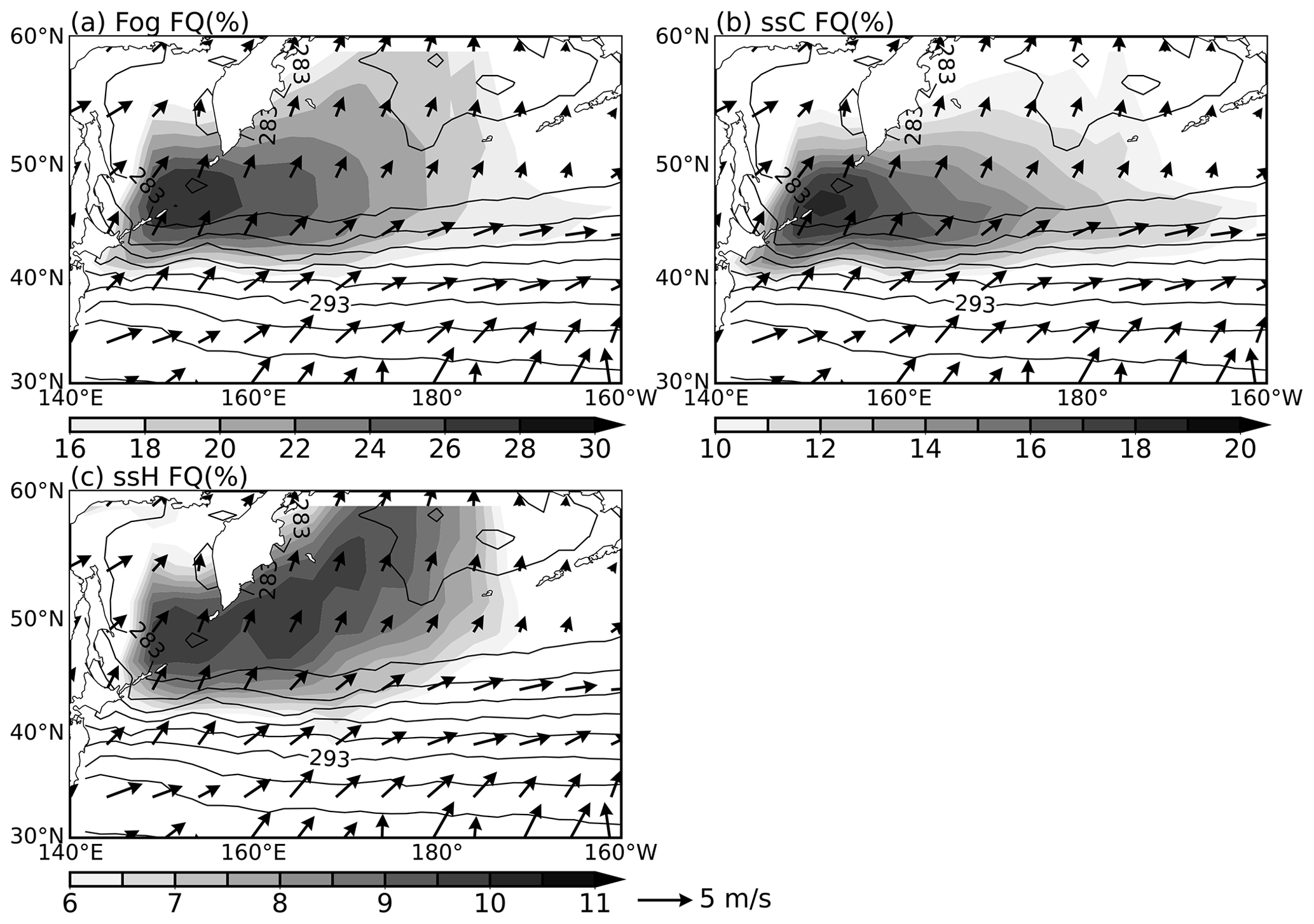
Figure 1 Climatological SST (contours with 2 K intervals), surface winds (vectors, m s⁻¹), and frequencies (shading, %) of (a) advection fog and advection fog with (b) SSC and (c) SSH during June–July–August for 1998–2018. The SST and winds are based on ERA5, and the fog frequencies are obtained from ICOADS.

Figure 2 illustrates the probability density function (PDF) of simultaneous SAT-SST values concurrent with advection fog over the NWP during JJA. The majority of these SAT-SST values are positive (Fig. 2), consistent with the observational results of Fu and Song (2014). However, a substantial proportion (∼ 27.5 %) of advection fog in the NWP is associated with SSH fog. Based on coastal buoy observations, Yang et al. (2019) reported that ∼ 30 % of SAT falls below SST during fog events in the Yellow Sea. Li et al. (2022) also observed that ∼ 32 % of fog is associated with SSH over the northeast Pacific during winter. The consistent observations of advection fog with SSH imply that cooling mechanisms other than near-surface turbulent cooling have a substantial impact on the evolution of advection fog.

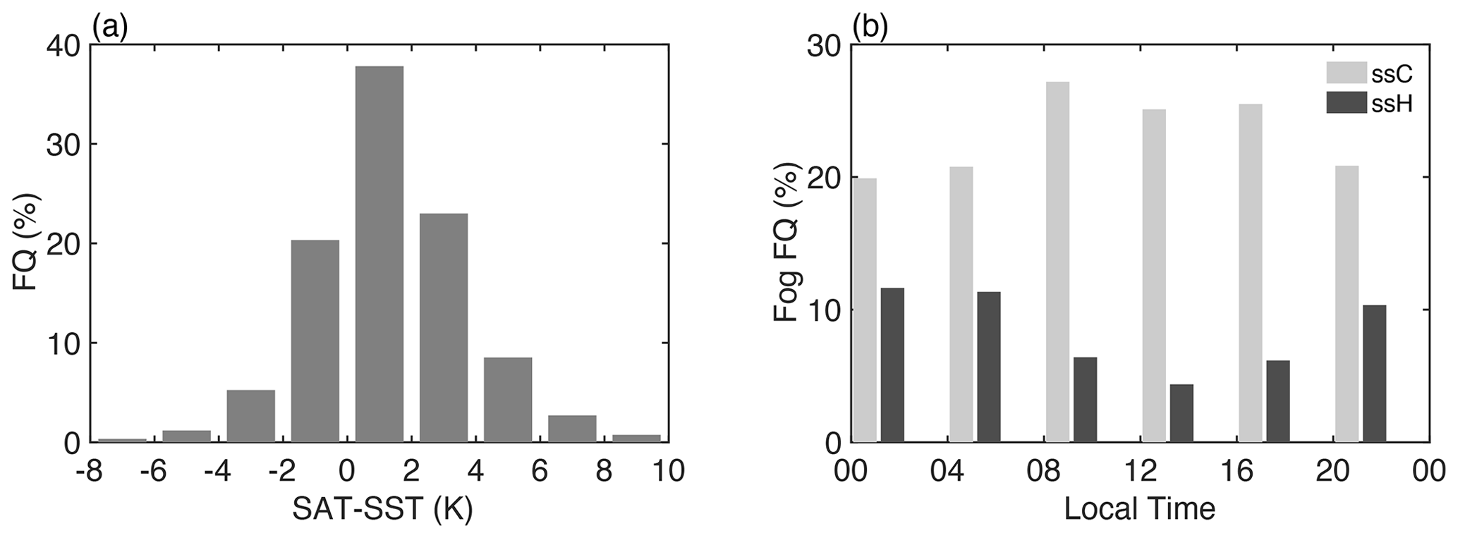
Figure 2 (a) Probability density function (%) of SAT-SST (°C) concurrent with advection fog observations over the NWP (30–60° N, 140–200° E) during June–July–August based on ICOADS. (b) The frequencies of advection fog with SSH (dark-grey bars) and SSC (light-grey bars) as functions of local time.

There is a noticeable diurnal variation in SSH fog over the NWP (the dark-grey bars in Fig. 2b). The local time is determined based on the universal time of fog observations and their respective longitudes. The frequency of SSH fog reaches its maximum (∼ 11.5 %) and minimum (∼ 4 %) during 00:00–04:00 and 12:00–16:00 local time, respectively (the dark-grey bars in Fig. 2b). Relative to all advection fog occurrences, the frequency of SSH fog is ∼ 18.8 % during the daytime and increases to ∼ 34.5 % at night. In contrast, the frequency of SSC fog is highest around sunrise (the light-grey bars in Fig. 2b) and does not exhibit a clear diurnal variation. The evident diurnal cycle of SSH fog over the open sea is new to our knowledge and suggests that the radiative balance over the fog top significantly alters the evolution of advection fog.

3.2 An SSH fog case

We examine an advection fog event during 1–4 July 2013 over the NWP. Satellite images observed by the Moderate Resolution Imaging Spectroradiometer (MODIS) captured clear fog patches at 10:00 local standard time (LST) during 1–3 July near the Kuril Islands and over the northwest Pacific (Fig. 3b). The synoptic steady southwesterlies over the SST front caused the fog event (Fig. 4), and ICOADS observations reported no precipitation during this period. Further information regarding this fog event can be found in Yang et al. (2021). Our primary focus is on the negative SAT-SST observations during this fog episode (Fig. 4). Fog was first reported near the Kuril Islands on the night of 30 June (red stars in Fig. 4b), concurring with positive SAT-SST. The southwesterly winds, along with positive SAT-SST, signify the event as advection fog. As the saturated air moved northeastward (Figs. 3b–d and 4e–h), negative SAT-SST was detected within the fog patch during 2–4 July (blue stars in Fig. 4e–h). Notably, most of the SSH fog occurred at night. Figure 5 shows the time series of observational SAT-SST closest to the trajectory in Fig. 4. After fog formation, there is a noticeable diurnal variation in the sea–air temperature difference, with air temperature dropping below SST during the nights of 2 and 3 July. The minimum sea–air temperature difference reaches −1 K at 22:00 LST on 3 July.

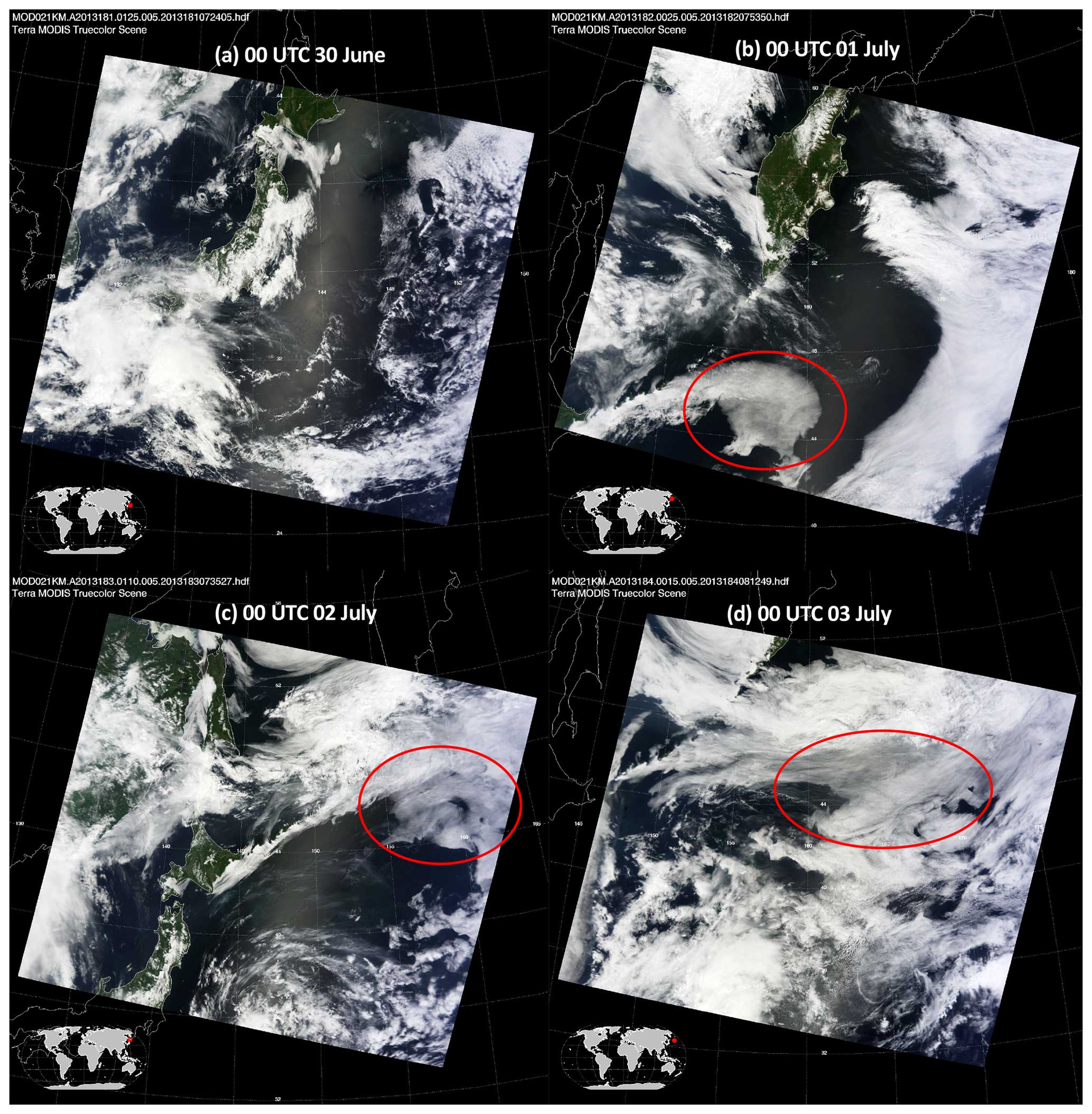
Figure 3 Visible satellite images from MODIS.

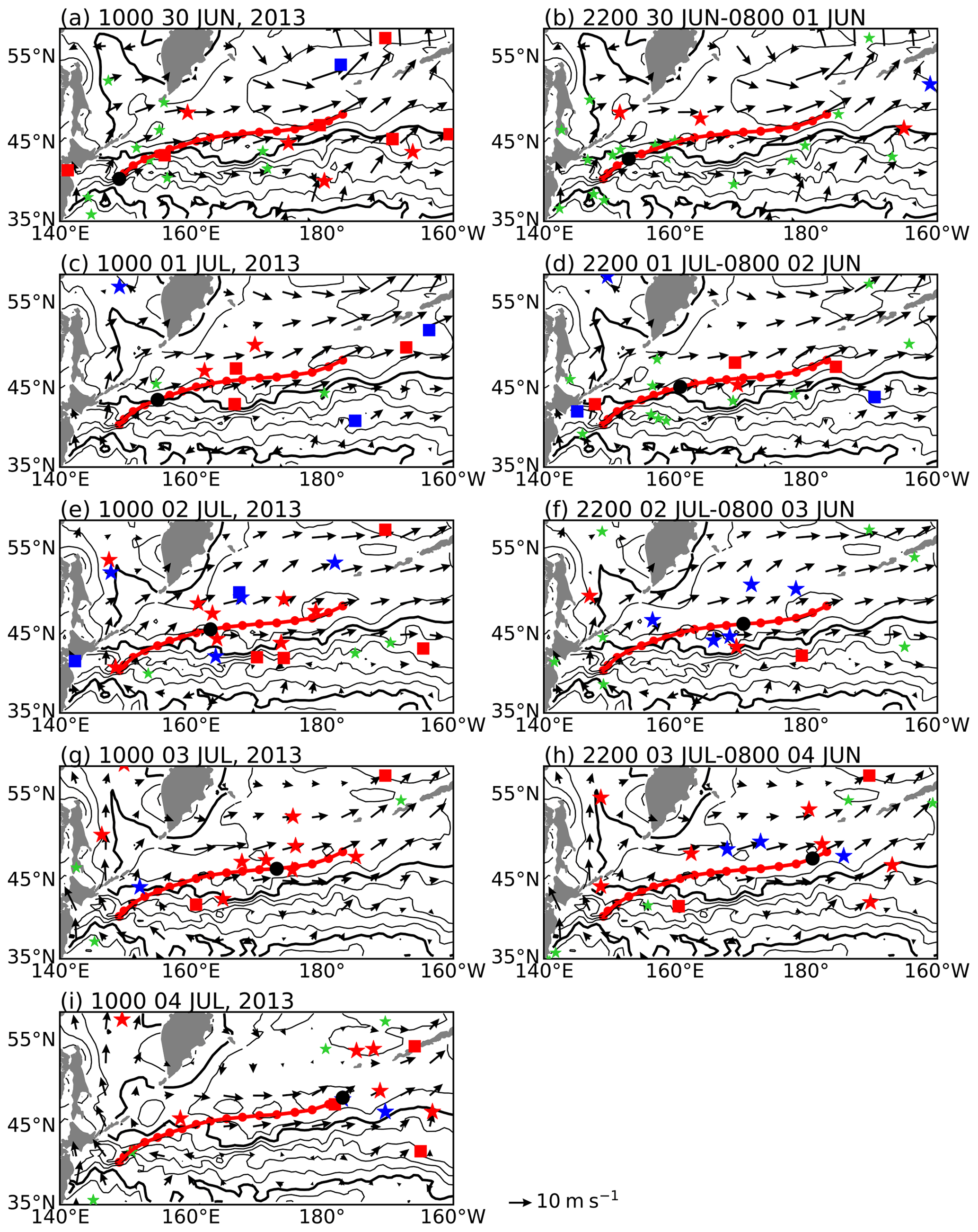
Figure 4 ICOADS observations of the advection fog event during 30 June–4 July 2013. The blue and red stars represent SSH and SSC fog, respectively, while the squares indicate stratus and the green stars indicate other cloud types or clear sky. The ICOADS observations and ERA5 10 m winds near 10:00 LST from 30 June to 4 July are shown in (a), (c), (e), (g), and (i), respectively. The ICOADS reports and ERA5 winds between 22:00–08:00 (+1 d) LST are shown in (b), (d), (f), and (h) to include more nighttime observations. The thick red line in each panel demonstrates the 4 d back trajectory from the SSH fog observation at 49.6° N, 183.2° E, and the red dots are the location of the trajectory every 6 h, with the larger black dot indicating the location at the corresponding time of the panel. The contours are averaged ERA5 SSTs during 30 June–4 July, and the thick contours indicate 283, 293, and 303 K.

4 Simulation with constant solar radiation

4.1 Simulation setups

The synoptic processes associated with the fog event detailed in Sect. 3.2 align closely with the climatological characteristics of SSH and SSC fog (Figs. 1 and 2). To uncover the boundary-layer processes responsible for the SSH fog, we use the UCLA-LES model to simulate this typical fog event from a Lagrangian perspective. We trace back an SSH fog observation at 49.6° N, 183.2° E in Fig. 4i, which had an SAT-SST value of −1.2 °C. This trajectory is roughly consistent with the one obtained using the HYSPLIT trajectory model (Draxler and Rolph, 2015; not shown). The air column consecutively experienced no fog, SSC, and SSH fog along the trajectory from 30 June to 4 July 2013 (Figs. 4 and 5).

We prescribe time-varying SST and large-scale divergence to force the boundary-layer evolution. To fit the observations, we simplify the observational SST by employing a cosine function during the initial 36 h, succeeded by a constant value of 8° (not shown). The fog case and the simulation setups are the same as those in Yang et al. (2021), except for the divergence forcing in the free atmosphere. We apply a realistic divergence of $\mathrm{2}\times {\mathrm{10}}^{-\mathrm{6}}$ s⁻¹, which is the averaged value along the trajectory and is double the climatological value in Yang et al. (2021). We first perform a simulation with fixed solar radiation.

We generate idealized initial conditions for the simulation by integrating ERA5 and satellite data. Cloud-Aerosol Lidar and Infrared Pathfinder Satellite Observations (CALIPSO) indicated a boundary-layer height of 400 m (not shown). We establish a typical clear-sky boundary-layer structure by linearizing the original ERA5 profiles into three parts: the mixed layer, inversion, and free troposphere. Within the 400 m deep mixed layer, the θ and q_t profiles remain constant (Fig. 7a and b). Above the mixed layer, an inversion with a 6 K jump in θ is present (Fig. 7a). In the free troposphere, θ and q_t decrease at the rate of −6.6 K km⁻¹ (Fig. 7a) and −4 g kg⁻¹ km⁻¹ (Fig. 7b), respectively. Throughout the simulation, winds of 9.6 m s⁻¹ in geostrophic balance are applied.

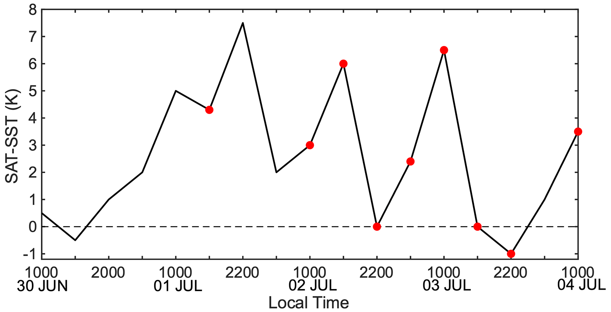
Figure 5 ICOADS observations of SAT-SST close to the trajectory in Fig. 4. The red dots indicate fog occurrences.

4.2 Evolution in the boundary-layer structure

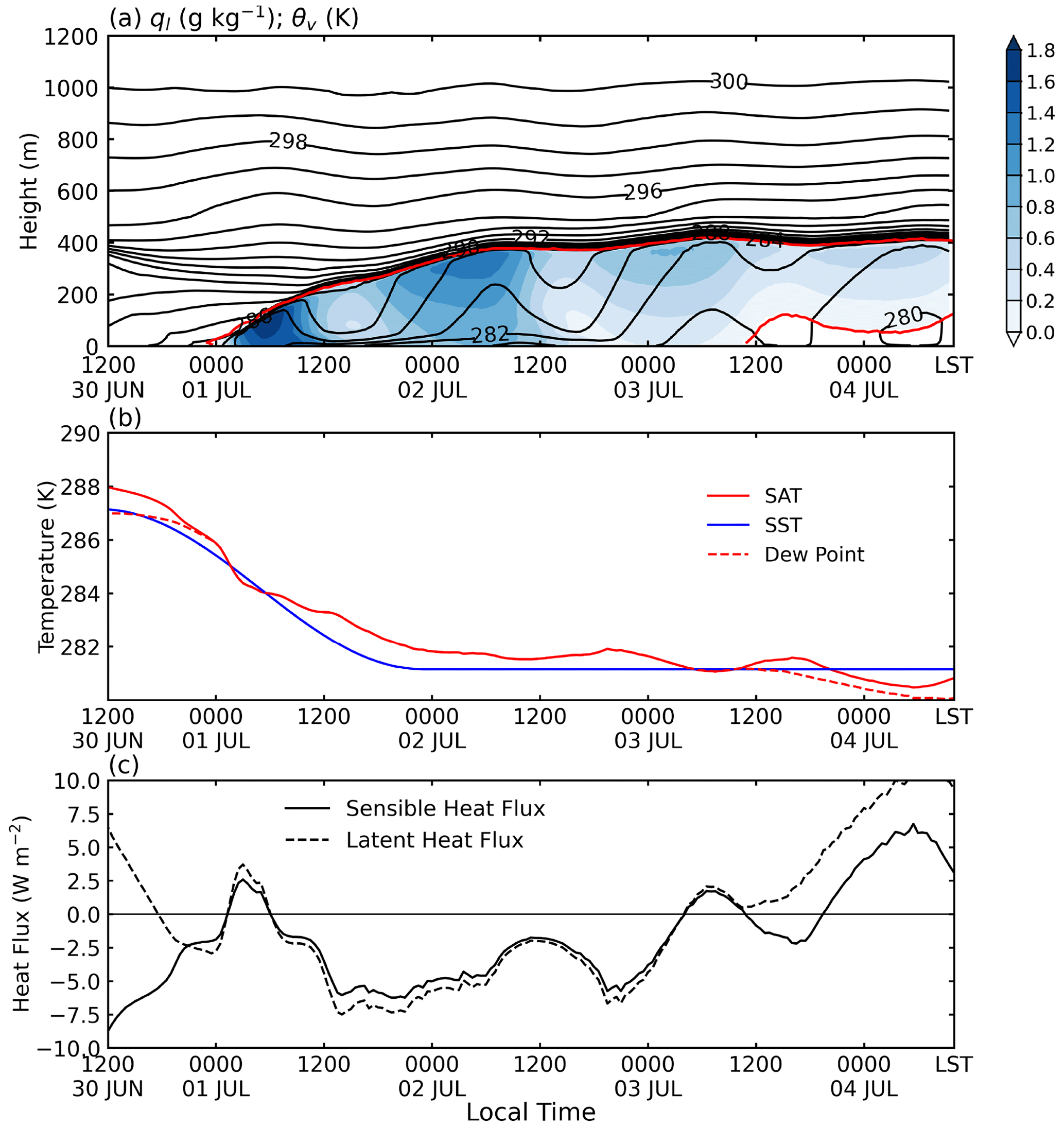
Figure 6a depicts the time–height section of the liquid water mixing ratio (q_l) and virtual potential temperature (θ_v) for the air column in the simulation with constant solar radiation. We exclude the first 2 h of results due to the model's spin-up. Liquid water initially appears near the surface (∼ 20 m) at 04:00 local standard time (LST) on 1 July and rapidly extends to the surface within 1 h, resulting in fog formation. We define fog when q_l exceeds 0.02 g kg⁻¹ (Kunkel, 1984). Fog persists until 02:00 LST on 4 July, transitioning into stratus as the near-surface droplets evaporate. This transition results from the entrainment of the free-atmospheric dry air caused by the fog-top LWC (Yang et al., 2021). The height of the fog top grows from 20 to 380 m until 00:00 LST on 3 July and rarely varies thereafter. CALIPSO passed through the fog area and observed cloud-top heights of about 300 and 400 m until 00:00 LST on 2 July and 01:00 LST on 3 July (not shown), respectively, which is very close to simulated results. The capping inversion intensifies from 5 to 12 K after fog formation due to the fog-layer cooling (Fig. 5a).

The model successfully reproduces the SSH fog. Over the SST front, SAT follows the underlying SST with a difference of 0.8 K, resulting in a strong downward sensible heat flux between −7.5 and 0 W m⁻² (Fig. 6b and c). At 04:00 LST on 1 July, SAT drops to the dew point at 285.8 K. After crossing the SST front, SAT is almost constant during the period of 00:00 LST on 2–3 July but quickly decreases afterward, falling below SST at 17:00 LST on 3 July (Fig. 6b). The occurrence time of SSH fog is consistent with ICOADS observations. The minimum air–sea temperature difference during sea fog is −0.65 K, weaker than the observed −1 K (Figs. 5 and 6b). From this time, both sensible and latent heat fluxes change their directions, indicating that the ocean begins to heat and moisten the surface air (Fig. 5b and c). The SSH fog sustains for 12 h.

We divide the simulation into four phases: fog formation (from 12:00 LST on 30 June to 04:00 LST on 1 July) and development (from 04:00 LST on 1 July to 00:00 LST on 2 July) over the SST front, followed by fog maintenance with SSC (from 00:00 LST on 2 July to 17:00 LST on 3 July) and SSH (from 17:00 LST on 3 July to 02:00 LST on 4 July) to the north of the SST front. Figure 6 shows the boundary-layer structure for the above four phases. The soundings of θ_v, the total water mixing ratio (q_t), and q_l are domain-averaged at the selected times.

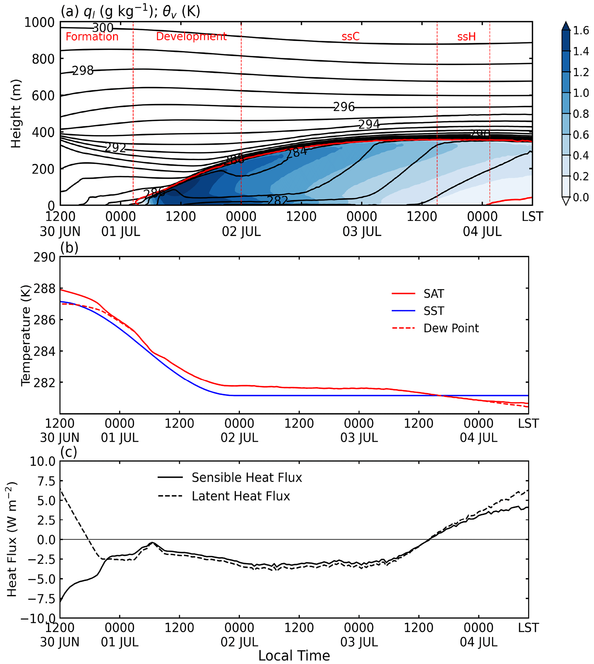
Figure 6 (a) Time–height section of simulated liquid water mixing ratio (shading, g kg⁻¹) and virtual potential temperature (contours, K) for a constant solar radiation simulation. Red lines indicate the fog/cloud top and bottom. (b) SAT (red line, K), SST (blue line, K), and surface dew point temperature (dashed red line, K). (c) Same as (b) but for surface sensible heat flux (solid line, W m⁻²) and latent heat flux (dashed line, W m⁻²). Upward sensible and latent heat fluxes are positive. Dashed red lines in (a) divide the evolution process of fog into the four phases described in the article.

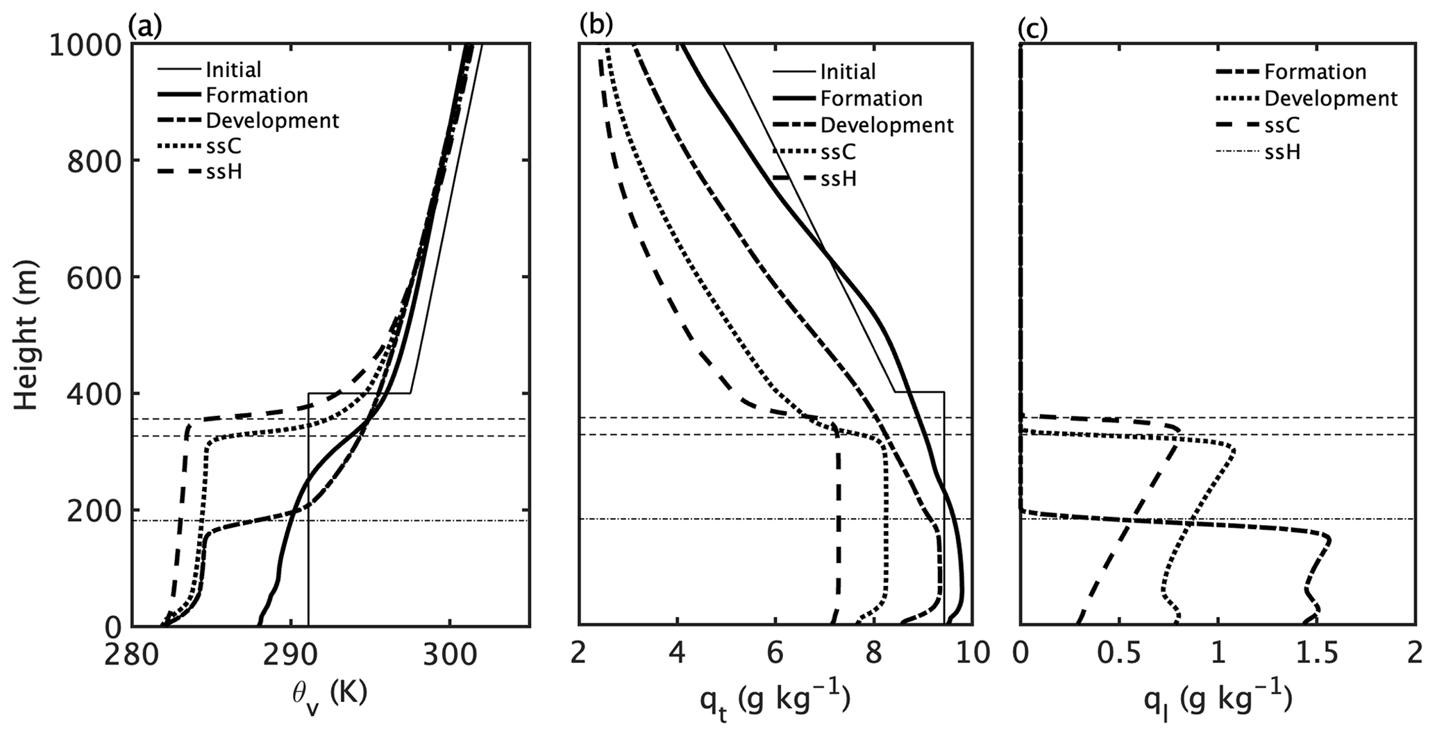
Figure 7 Horizontal mean soundings for constant solar radiation simulation at 10:00 LST on 30 June (thin solid line), 20:00 LST on 30 June (solid line), 12:00 LST on 1 July (dot-dashed line), 12:00 LST on 2 July (dotted line), and 20:00 LST on 3 July (dashed line). (a) Virtual potential temperature (K), (b) total water mixing ratio (g kg⁻¹), and (c) liquid water mixing ratio (g kg⁻¹). Horizontal dot-dashed line represents the fog-top height at 12:00 LST on 1 July, and the horizontal dashed line represents the fog-top heights at 12:00 LST on 2 July and 20:00 LST on 3 July.

Before fog formation, the cold sea surface efficiently cools the near-surface air, creating a stable boundary layer (Figs. 6a and 7a). q_t increases with height below 20 m and remains nearly constant within the boundary layer (Fig. 7b). The upward decrease in air temperature and increase in q_t result in the maximal relative humidity and saturation occurring near 20 m (Fig. 7a). Once fog forms, a mixed layer develops downward from the fog top to 50 m, capping the original stable layer produced by the cold sea surface (Fig. 7a). θ_v and q_t of the boundary layer decrease by ∼ 6 K and ∼ 1 g kg⁻¹, respectively, from 20:00 LST on 30 June to 12:00 LST on 1 July (Fig. 7a and b). Large q_l near the fog top converts into rainwater and descends, resulting in a secondary peak of q_l near the surface at about 20 m (Fig. 7c). The stratifications of θ_v, q_t, and q_l indicate a different cooling mechanism at the fog top from that at its bottom (Fig. 7a).

During the SSC fog phase, a well-mixed boundary layer develops, and θ_v decreases by 1 K from 12:00 LST on 1 July to 12:00 LST on 2 July (Fig. 7a and b). q_l peaks near the fog top (Fig. 7c). During the SSH fog phase, the sea surface heats and moistens the fog layer (Fig. 6b) while the fog layer keeps cooling and drying at a much slower rate (Fig. 7a), indicating that the LWC effect at the fog top dominates the fog cooling and maintenance. The thermal and moisture stratifications of SSH fog share a similar structure to those of SSC fog but with a deeper well-mixed layer (the long dashed lines in Fig. 7).

4.3 Heat and moisture budgets

Figure 8 shows the profiles of heat and water vapor budget terms at different phases. Figure 9a and b show the time series of surface heat and water vapor budget terms, respectively. Over the SST front, the turbulent mixing and longwave radiation effects cool the air both near the surface and throughout the entire boundary layer (Figs. 8a and 9a). Fog forms due to the cooling of the air near the surface (Fig. 8a).

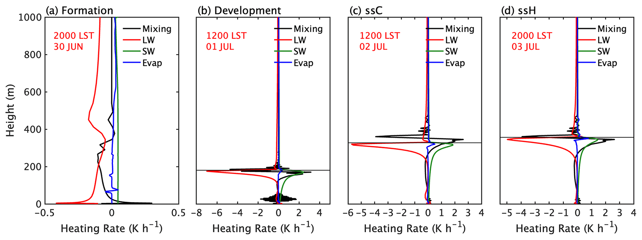
Figure 8 Profiles of horizontal mean budget terms for heat (K h⁻¹) at (a) 20:00 LST on 30 June, (b) 12:00 LST on 1 July, (c) 12:00 LST on 2 July, and (d) 20:00 LST on 3 July in the constant solar radiation simulation. The horizontal lines indicate the fog tops.

After fog formation, the surface turbulent cooling intensifies dramatically, peaking at −1.35 K h⁻¹, leading to a marked decrease in SAT (Fig. 9a). The rapid growth of q_l releases latent heat through condensation, which partly offsets the cooling effect from turbulent mixing. Caldwell and Bretherton (2005) suggested that sedimentation has a drying and heating effect on the surface layer. The impact of sedimentation for the heat budget is relatively small compared to turbulent mixing and LWC, both at the surface and within the boundary layer (not shown). Within the boundary layer, the longwave radiation effect induces strong cooling at the fog top, and the resultant turbulent mixing cools the upper boundary layer (the red line in Fig. 8b). Additionally, thermal turbulence helps entrain the warm, dry air from the free atmosphere, warming the air at the fog top while cooling the air above the fog layer (the black line in Fig. 8b).

When the fog volume moves north of the SST front (00:00 LST on 2 July onward), the surface-cooling effects become weak due to the fixed SST and turbulent mixing drying the surface air (Fig. 9). Strong LWC persists at the fog top, inducing turbulent mixing that cools the entire fog layer (Figs. 7a and 8c). In this case, the effect of the fog-top LWC overcomes the surface-cooling effect, causing SAT to drop below SST. During the SSH phase, the LWC at the fog top slightly weakens and the turbulent mixing cooling dominates within the fog layer, causing SAT to continuously decrease (Figs. 6b and 8d).

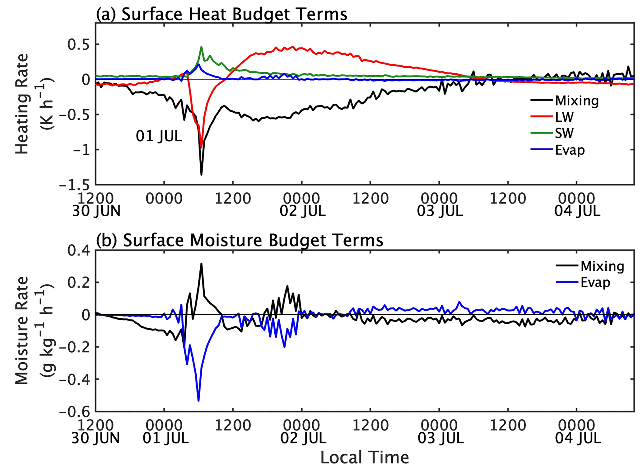
Figure 9 Time series of horizontal mean budget terms at the surface for the constant solar radiation simulation: (a) heat (K h⁻¹) and (b) water vapor (g kg⁻¹ h⁻¹).

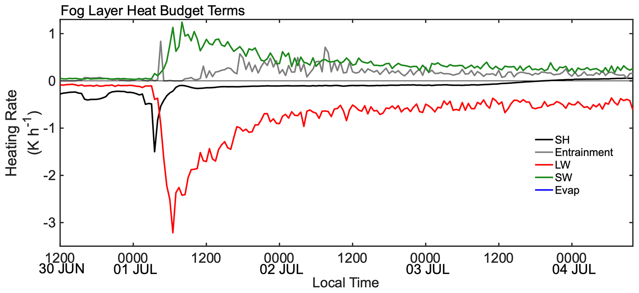
Figure 10 Time series of horizontal mean heat budget terms (K h⁻¹) of the integral boundary layer for the constant solar radiation simulation.

We quantify the heat budget for the fog layer by integrating the heat budget for the fog layer (Fig. 10). We determine the turbulent mixing term by calculating the difference between the turbulent heat fluxes at the surface (${\stackrel{\mathrm{‾}}{w{}^{\prime }\mathit{\theta }{}^{\prime }}}_{\mathrm{sfc}}$) and the fog top (${\stackrel{\mathrm{‾}}{w{}^{\prime }\mathit{\theta }{}^{\prime }}}_{z_i}$; z_i is the fog-top height), representing the surface sensible heat transport and the effect of the fog-top entrainment, respectively (the black and grey lines in Fig. 10). Prior to fog formation, the surface sensible heat transport drives the boundary-layer cooling (the black line in Fig. 10). After the fog forms, the effect of longwave radiation acts to cool the boundary layer due to the longwave heat loss at the fog top (the red line). The LWC effect rapidly exceeds surface cooling 2 h after fog formation. Both shortwave radiation and entrainment at the fog top warm the fog layer, partially offsetting the effects of surface cooling and LWC.

The normalized LWC by the fog-layer depth peaks 6 h after fog formation and then decreases rapidly (Fig. 10). This is possibly related to a negative feedback between the fog-top radiative cooling and entrainment (Gerber et al., 2013, 2014). Following the fog formation, an increase in fog-top entrainment causes a reduction in the liquid water gradient at the fog top, which subsequently reduces the radiative cooling. This negative feedback process takes several hours to take effect (not shown). Another reason for the initial surge in LWC is the rapid growth of fog-layer depth. In addition, we examine the time series maximum in LWC profiles (not shown), which fluctuates around 8 K h⁻¹ after fog formation and then steadily decreases. The fog-top LWC is somewhat less than the counterpart for typical stratocumulus clouds (Curry and Herman, 1985; Gerber et al., 2014). This may be attributed to the difference in free-atmospheric humidity between fog and stratocumulus scenes. In the case of stratocumulus clouds, the corresponding descending motion results in drier air compared to the free atmosphere above fog. As the fog moves to the cold flank of the SST front, the surface cooling weakens and reverses, slightly heating the fog layer after SAT drops below SST. Overall, the persistent and strong LWC at the fog top dominates the fog evolution, resulting in the SSH fog.

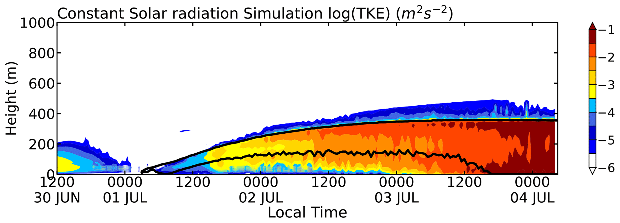
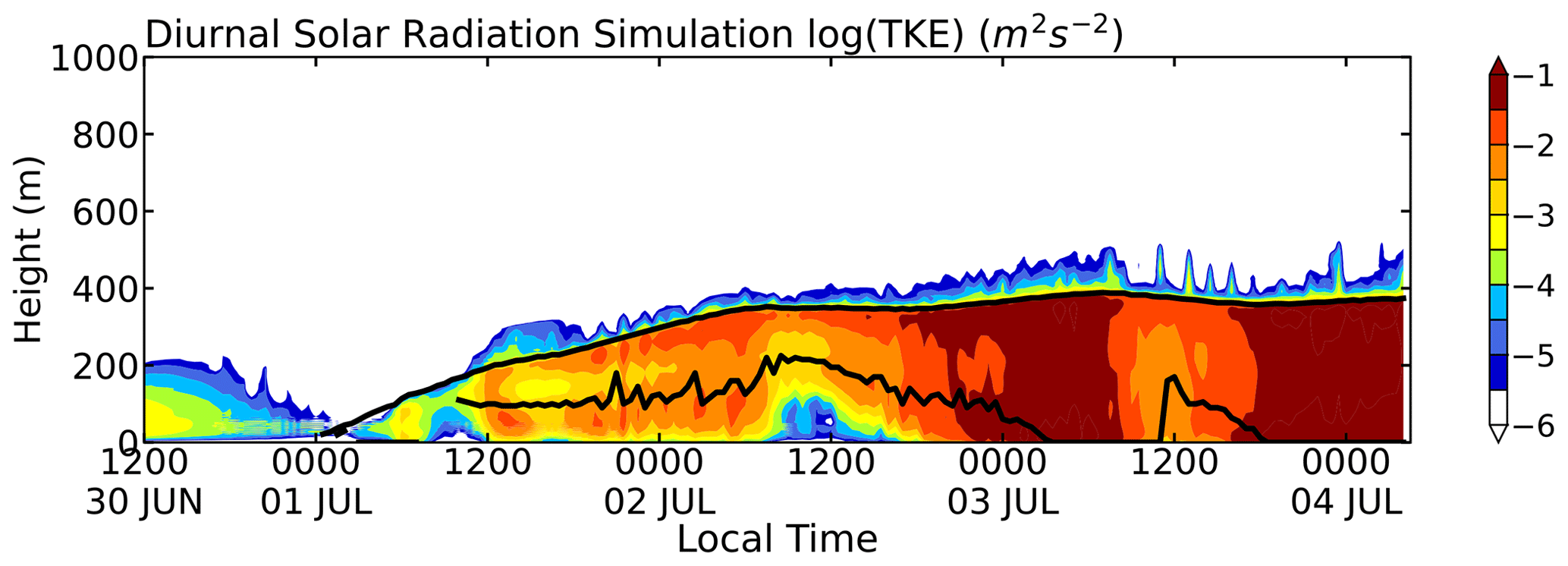
Figure 11 Time–height section of log₁₀ (TKE) (shading in m² s⁻²) and time series of fog/cloud top height (upper black lines in m) and the thermal-turbulence interface (lower black lines in m) for the simulations with constant solar radiations.

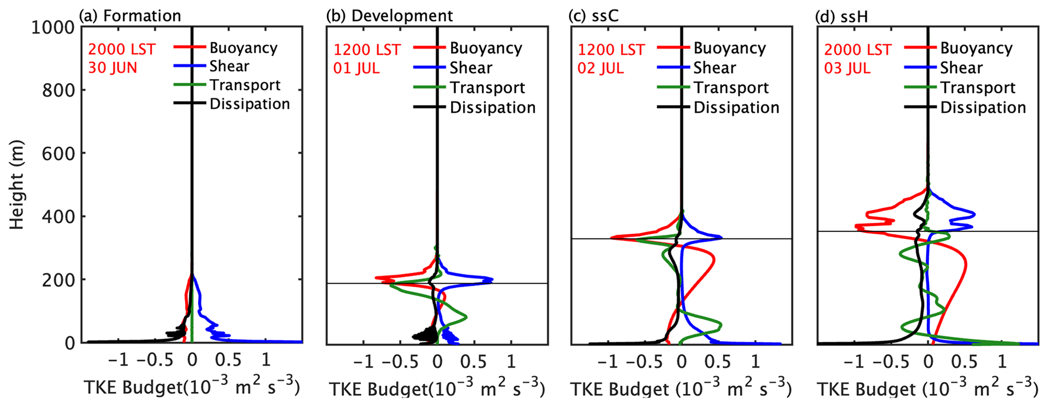
Figure 12 Profiles of horizontal mean TKE budget terms (10⁻³ m² s⁻³) for the constant solar radiation simulation at (a) 20:00 LST on 30 June, (b) 12:00 LST on 1 July, (c) 12:00 LST on 2 July, and (d) 20:00 LST on 3 July. Thin black lines indicate the fog tops.

4.4 TKE and its budget

Figure 11 presents the time–height cross section of TKE for the simulation with constant solar radiation. Prior to fog formation (04:00 LST on 1 July), TKE exhibits a relatively low magnitude below 200 m (Fig. 11), produced by the near-surface wind shear and dissipated by friction and buoyancy (Fig. 12a). Mechanical turbulence facilitates the transport of cooling from the surface, contributing to the fog formation. Following fog formation, the LWC at the fog top induces buoyancy production of turbulence over the upper boundary layer (Fig. 12b), leading to a noticeable peak in TKE near the fog top ∼ 12 h after its formation (Fig. 11).

Turbulence in the SSC fog intensifies after its formation at 00:00 LST on 2 July (Fig. 11). The terms in the TKE budget also exhibit a general strengthening trend from fog formation to the SSC fog (Fig. 12c). The generation of buoyancy-driven turbulence enhances and develops downward, leading to a deeper mixing layer within the boundary layer and cooling fog layer (Figs. 7a and 12c). TKE exhibits a significant increase from the SSC fog to SSH fog, particularly near the surface. This is because the air–sea interface becomes unstable (SAT-SST < 0), leading to the buoyancy production of turbulence (Fig. 12d). During this period, both buoyancy-induced and mechanically induced turbulence contribute significantly to the maximum TKE near the surface.

The vertical structure of turbulence can be elucidated by employing the thermal-turbulence interface, which distinguishes between the layers characterized by thermal and mechanical turbulence (Huang et al., 2015). Huang et al. (2005) defined a thermal-turbulence interface as the gradient of the observational potential pseudo-equivalent temperature equals zero. Thermal turbulence induced by LWC is prevalent above the thermal-turbulence interface, which is static unstable, whereas mechanical turbulence, aroused by wind shear, is predominant below the interface. A thermal-turbulence interface helps to separate the fog layer into zones dominated by LWC and surface cooling. In this article, the thermal-turbulence interface is defined as the lowest altitude within the fog layer where the buoyancy production of turbulence is positive (the black lines in Fig. 11). Following fog formation, a thermal-turbulence mixing layer forms beneath the fog top and extends across the upper half of the fog layer from 00:00 LST on 2 July (Fig. 11). After 00:00 LST on 3 July, the mixing layer continues to develop downward, eventually reaching the sea surface by 15:00 LST on the same day, thus establishing a well-mixed boundary layer. Subsequently, the thermal turbulence cools the near-surface air and causes SAT to drop below SST after a 2 h interval (Fig. 6b).

Figure 13 As in Fig. 6 but for the simulation with diurnal-cycle radiation.

Figure 14 As in Fig. 11 but for the simulation with diurnal-cycle radiation.

5 Simulation with diurnal solar radiation

We conduct an additional simulation that incorporates diurnal solar radiation. Overall, the simulated fog with diurnal solar radiation exhibits similar behavior to that in the simulation with constant solar radiation but with clear diurnal variations. Fog forms at 22:00 LST on 30 June and rapidly grows. During the night, the stronger fog-top LWC enhances thermal turbulence and entrainment, causing an increase in the fog-top height (Fig. 13a). In contrast, during the day, fog height decreased noticeably (Fig. 13a). With the continued drying effect of entrainment, liquid water content in the fog layer decreases, ultimately causing the transition from fog to stratus at 11:00 LST on 3 July (Fig. 13a).

The simulation incorporating diurnal solar radiation also generates SSH fog, which exhibits significant diurnal variation. During the nights of 3 and 4 July, SAT rapidly drops below SST after sunset and recovers above SST after sunrise, which is similar to the variations in observational SAT-SST (Figs. 5 and 13b). This result indicates that the diurnal variation in the radiative balance over the fog top considerably alters the transitions between SSC and SSH fog. The LWC at the fog top has a clearer diurnal variation and dominates the air–sea temperature differences (not shown). About 3–5 h before sunset, the fog-top LWC reaches its minimum during the day. The enhancement of LWC occurs approximately 3 h earlier than the decline in air–sea temperature difference, ultimately causing the air temperature to fall below SST in the early hours of 3 July (not shown). Additionally, both TKE and the thermal-turbulence mixing layer exhibit distinct diurnal variations (Fig. 14). The pronounced radiative cooling at the fog top results in increased TKE and a thicker thermal-turbulence mixing layer at nighttime compared to daytime (Fig. 14). The time period when the mixing layer base and the ground coincide is the same as the occurrence period of SSH fog, further demonstrating the regulating effect of LWC on the fog-layer cooling.

We also conducted a simulation with intensified solar irradiance through an increase in solar elevation angle to check the effect of solar irradiance. Sea fog dissipates 8 h earlier than it does in the standard solar radiation experiment and observations (not shown); 2 h before sea fog dissipation, there is the SSH fog occurrence. Nevertheless, there are minimal changes in the evolution of the fog-top height and the thermal and dynamic structure of the boundary layer during sea fog.

6 Summary and discussion

Sea fog is of great importance due to its significant impact on maritime activities. The present study synthesizes the long-term shipborne observations and a LES model to explore the phenomena of negative SAT-SST during advection fog over the NWP (referred to as SSH fog). The UCLA-LES model successfully simulates a fog event with SSH fog and captures the diurnal variation in SAT-SST during the fog episode. The simulation results highlight the strong influence of the LWC effect at the fog top on the formation of SSH fog.

Long-term shipborne observations reveal the prevalence of advection fog along the cold flank of the SST front in the NWP during the boreal summer. The SSH fog often occurs downstream of the regime of the advection fog with positive SAT-SST. The relative frequency of SSH during episodes of advection fog is ∼ 27.5 % in JJA, which is roughly consistent with the results over the summertime Yellow Sea (Yang et al., 2021) and wintertime northeast Pacific (Li et al., 2022). Furthermore, our findings reveal, for the first time, that the relative frequency of SSH fog exhibits a distinct diurnal cycle, with a peak occurrence (∼ 34.5 %) before sunrise and a trough occurrence (∼ 18.8 %) in the afternoon (Fig. 2b). This suggests that the thermal dynamics and associated turbulence structure of advection fog exhibit significant diurnal variation.

From a Lagrangian perspective, we utilize the turbulence-closure UCLA-LES model to simulate an advection fog event over the NWP from 1 to 4 July 2013, which exhibits similar characteristics to the observations of this sea fog case and long-term features of SSH fog. Surprisingly, the LES model successfully reproduces the diurnal variation in SAT-SST of the observations when incorporating diurnal solar radiation, indicating that the model captures the essential processes responsible for SSH fog.

We analyzed the LES with constant solar radiation in detail, which also produces SSH fog during the advection fog episode. Before the fog formation, the decreased SST over the oceanic front cools the near-surface air through the mechanical turbulence and triggers fog occurrence. Around the fog initiation, the cold sea surface drives a stable layer below 40 m in altitude, which decouples the fog layer from the sea surface. Once the surface vapor condenses, in the perspective of the fog layer, the fog-top LWC effect rapidly exceeds the near-surface mechanical cooling within ∼ 2 h of the fog formation (Fig. 9) when the air column is still on the SST front. A thermal-turbulence interface, separating the layers characterized by thermal and mechanical turbulence, effectively depicts the evolution of the vertical turbulence structure (Fig. 10a). The thermal turbulence from the fog top gradually develops downward to transport the fog-top LWC effect and reaches the surface 43 h after the fog formation, leading to the SAT drops below SST. The occurrence time of SSH fog and minimum SAT-SST (−0.65 K) is close to the observation result (−1 K).

In the LES with diurnal-cycle radiation, the enhancement of LWC during nighttime causes the thermal-turbulence interface to reach the surface, leading to the occurrence of SSH fog. In the daytime, the thermal-turbulence interface moves away from the surface and the SAT rises above the SST due to weakened LWC. This result is consistent with the observed variations in SAT-SST, while the simulated SAT-SST is weaker than the observations. This suggests that the LWC is underestimated in the model, which could be related to the model vertical resolution.

Previous studies have primarily focused on the diurnal variation in fog frequency using observational data and models (O'Brien et al., 2013; Liu et al., 2021), but there has been a lack of research on the diurnal variation in air–sea temperature difference. The reason is that sea fog evolution is not as strongly influenced by the diurnal variation in surface temperature as radiation fog on land (Koračin and Dorman, 2017); there is a weak variability in SST during sea fog episodes. Kim and Yum (2013) investigated the effect of the diurnal variation in radiation on advection fog formation by the PAFOG model, but they did not discuss the diurnal variation in SAT-SST during fog due to the fog period being short. This paper verifies, from both observational and modeling perspectives, that sea fog exhibits significant diurnal variations in air–sea temperature difference, primarily regulated by LWC at the fog top and thermal turbulence.

Our LES results suggest that SSH fog formation is characterized by a thermal-turbulence layer, induced by the LWC at the fog top, that pervades the entire fog layer and cools the near-surface air below the sea surface temperature (SST). Previous studies primarily used the near-surface liquid water in sea fog to validate the weather model performance in simulating sea fog (e.g., Gao et al., 2007; Y. Yang et al., 2018). Considering the limited availability of observations on the vertical structure of fog over the open sea, the observations of air–sea temperature differences during advection fog events offer valuable insights for improving the modeling of the thermal turbulence induced by the LWC at the fog top. The presence of SSH fog signals a pronounced LWC at the fog top and thorough mixing of thermal turbulence within the layer. Consequently, refining weather models to account for air–sea temperature differences enables more precise sea fog simulations, especially in terms of the thermal turbulence within the fog layer. For instance, Yang et al. (2019) used a top-down mixing parameterization in the WRF model to characterize turbulence from the fog top. The thermal turbulence is explicitly resolved in UCLA-LES. Comparing these models' simulation results may refine the turbulence parameterization in weather models, which is a desirable aim for future research.

Yang et al. (2021) applied a weaker subsidence and did not simulate SSH fog. Our simulation results demonstrate that descending motion plays an important role in modulating the LWC at the fog top. Thus, stronger descending motion leads to a longer fog duration (72 h vs. 55 h in Yang et al., 2021) and a lower fog-top height (380 m vs. 580 m in Yang et al., 2021). These findings indicate that large-scale descending motion modulates the characteristics of fog by altering the fog-top LWC.