Investigating long-term changes in polar stratospheric clouds above Antarctica during past decades: a temperature-based approach using spaceborne lidar detections

Polar stratospheric clouds play a significant role in the seasonal thinning of the ozone layer by facilitating the activation of stable chlorine and bromine reservoirs into reactive radicals, as well as prolonging the ozone depletion by removing HNO₃ and H₂O from the stratosphere by sedimentation. In a context of climate change, the cooling of the lower polar stratosphere could enhance polar stratospheric cloud (PSC) formation and by consequence cause more ozone depletion. There is thus a need to document the evolution of the PSC cover to better understand its impact on the ozone layer. In this article we present a statistical model based on the analysis of the CALIPSO (Cloud–Aerosol Lidar and Infrared Pathfinder Satellite Observations) PSC product from 2006 to 2020. The model predicts the daily regionally averaged PSC density by pressure level derived from stratospheric temperatures. Applied to stratospheric temperatures from the CALIPSO PSC product, our model reproduces observed and interannual variations in PSC density well between 10 and 150 hPa over the 2006–2020 period. The model reproduces the PSC seasonal progression well, even during disruptive events like stratospheric sudden warmings, except for years characterized by volcanic eruptions. We also apply our model to gridded temperatures from Modern Era Retrospective analysis for Research and Application (MERRA-2) reanalyses over the complete South Pole region to evaluate changes in PSC season duration over the 1980–2021 period. We find that over the 1980–2000 period, the PSC season gets significantly longer between 30 and 150 hPa. Lengthening of the PSC season from 22 d (30–50 hPa) to 32 d (100–150 hPa) is possibly related to volcanic eruptions occurring over this period. Over 1980–2021, we find that the PSC season gets significantly longer between 30 and 100 hPa, but due to biases in MERRA-2 temperatures, the reliability of these trends is hard to evaluate.

1 Introduction

In the 1980s, the attention of the scientific community was captured by the discovery of a hole in the ozone layer. Research revealed that ozone thinning is driven by the presence of chlorine (Molina and Rowland, 1974) that is mainly emitted by human activities in the form of chlorofluorocarbons (CFCs), which due to their long lifetime persist in the atmosphere for a long time. Photolysis, a chemical reaction triggered by sunlight, converts the CFCs into active chlorine, which then reacts with ozone, leading to its depletion. However, the high levels of chlorine observed at the poles could not be entirely explained by the presence of CFCs alone (Solomon et al., 1986). Polar stratospheric clouds (PSCs) emerged as a significant contributor to this phenomenon.

PSCs form in the polar stratosphere between 15 and 30 km in altitude during hemispheric winters when the polar vortex lowers the stratospheric temperature sufficiently (T < 195 K) to enable their formation. Cold temperatures trigger chemical nucleation processes involving water vapor (H₂O), nitric acid (HNO₃), and sulfuric acid (H₂SO₄), causing the formation of three types of particles that are often mixed within PSCs. (1) Liquid droplets of supercooled ternary solution (STS) form when water vapor and nitric acid condense on stratospheric background aerosols. (2) Solid particles of nitric acid trihydrate (NAT) exclusively form through heterogeneous nucleation processes, occurring either on ice particles or meteoritic nuclei (e.g., Hoyle et al., 2013; James et al., 2018). The nucleation of NAT particles on meteoritic nuclei was first documented by laboratory studies (e.g., Bogdan et al., 2003). Observations showed that despite an absence of stratospheric dehydration and temperatures above the freezing point, low-density, large NAT particles known as “NAT rock” or “mother NAT” can form (Tritscher et al., 2021). (3) Ice crystals also form in the polar stratosphere through both homogeneous and heterogeneous nucleation. Homogeneous nucleation is well-understood and requires extremely low temperatures (3–4 K below the freezing point). These can be generated by gravity waves triggered by orography and lead to the fast formation of a specific PSC type known as wave ice PSC. NAT particles can nucleate on these ice particles and propagate over vast regions, a phenomenon called the “NAT belt” (e.g., Höpfner et al., 2006). Heterogeneous nucleation of ice PSC particles can occur over pre-existing NAT particles (Fortin et al., 2003) or foreign nuclei. Even though temperatures are key in driving the formation of specific PSC particles, other parameters are important, for instance water vapor: studies have shown that a wetter and cooler stratosphere would produce more PSC (e.g., Stenke and Grewe, 2005; Khosrawi et al., 2016). Even if measurements suggest stratospheric water vapor could have increased locally since 1980, satellite data records show little overall net change since then (Hegglin et al., 2014). According to the AR6 report there is low confidence in trends of stratospheric water vapor over the era of satellite observation (IPCC, 2021).

PSCs have a dual role in the thinning of the ozone layer. First, by being the site for heterogeneous reactions, they activate the stable reservoirs of chlorine and bromine of the stratosphere into free radicals which subsequently interact with ozone and contribute to its destruction during polar spring with the return of sunlight (Solomon, 1999). Secondly, solid PSC particles by the uptake of the HNO₃ and H₂O have the potential to grow to larger sizes and settle out of the stratosphere. This sedimentation induces the denitrification and dehydration of the stratosphere, which delays the deactivation of chlorine and thus prolongs the ozone depletion (e.g., Toon et al., 1986; Jensen et al., 2002; Khosrawi et al., 2017). Although since the implementation of the Montreal Protocol ozone-depleting substances like CFCs have decreased (Montzka et al., 2003), fluctuations in stratospheric temperatures also influence the future recovery of stratospheric ozone (Eyring et al., 2007). Indeed, the rate of chemical reactions causing ozone destruction and PSC formation is temperature-dependent (e.g., Hanson and Mauersberger, 1988; Marti and Mauersberger, 1993). Moreover, the increasing trend in greenhouse gases (GHGs) due to anthropic emissions induces a cooling effect of the lower stratospheric levels (AR6, IPCC, 2021) which could enhance PSC formation, resulting in increasing ozone depletion despite a decrease in stratospheric chlorine loading (Shindell et al., 1998). Equilibrium-doubled CO₂ experiments in different models and experimental setups confirmed this trend by predicting a cooler stratosphere (Wang et al., 2020). It is therefore crucial to document the PSC cover and understand what drives its evolution in a context of climate change to better understand its impact on the reformation of the ozone hole.

Our goal is to better understand if changes in PSC cloud cover over climate timescales could potentially affect the reformation of polar stratospheric ozone. To make progress toward this goal, our objective in this paper is to evaluate if the seasonal evolution of PSC over Antarctica has gone through significant changes over the past decades (1980–2021). We first use PSC detections obtained from spaceborne lidar measurements between 60 and 82° S over the 2006–2020 period to develop a statistical model that predicts by pressure level the daily average PSC density over the polar region based on stratospheric temperatures. We apply this model to a gridded dataset of stratospheric temperatures from reanalyses that cover the entire Antarctica region (60–90° S) to evaluate seasonal PSC changes over the past decades.

We first present the data used for our study in Sect. 2, including observations and reanalysis. Section 3 outlines the methodology to create our statistical model. In Sect. 4, we verify the robustness of our model by comparing the observed evolution of PSC density, as measured by spaceborne CALIPSO (Cloud–Aerosol Lidar and Infrared Pathfinder Satellite Observations) from 2006 to 2020, with the estimated PSC density generated by our model. In Sect. 5, we apply our model to the gridded stratospheric temperatures from reanalysis covering the years 1980 to 2021, allowing us to document the evolution of PSC seasons. In Sect. 6, we discuss the influence of sudden stratospheric warmings and volcanic eruptions on our model predictions. Section 7 consists of a discussion and conclusion based on the results obtained in the study.

2 Data

2.1 Spaceborne lidar PSC product

From 2006 to 2018, CALIPSO (Cloud–Aerosol Lidar and Infrared Pathfinder Satellite Observations) was part of the A-Train, a constellation of satellites flying at an altitude of 705 km above sea level (a.s.l.) along a sun-synchronous polar orbit inclined at 98° (Winker et al., 2009). In 2018, CALIPSO moved to a lower orbit called the C-Train, 16.5 km lower (Braun et al., 2019). CALIPSO crossed the Equator 15 times per day and provided coverage between 82° N and 82° S, making it a satellite of interest for the study of the polar regions. CALIPSO ended operations in July 2023.

The main CALIPSO instrument is CALIOP (Cloud–Aerosol LIdar with Orthogonal Polarization), a two-wavelength lidar (532 and 1064 nm) which measures polarized backscatter from atmospheric components. Here we use the CALIPSO PSC product level 2 (LID_L2_PSCMask-Standard-V2-00), obtained by applying the V2 PSC detection and composition classification algorithm to CALIOP level 1B data as described in Pitts et al. (2009, 2018). This product describes the spatial distribution, composition, and optical properties of PSC layers along the CALIPSO orbit track. The product is presented as daily files. Each daily file contains vertical profiles every 5 km along-track, each containing 121 altitude levels between 8 and 30 km a.s.l. with a vertical resolution of 180 m. In the product, from May to October, daily files contain profiles sampled over the South Pole region (50–82° S), and from December to March daily files contain profiles sampled over the North Pole region (50–82° N). Here, we focus only on the South Pole (May–October). The product includes complementary information, such as the temperature from reanalysis (Sect. 2.2) interpolated on the PSC data product grid.

In the CALIPSO PSC product, PSC detection is limited to nighttime observations as they ensure a high signal-to-noise ratio. This means the PSC sampling changes along a season (Appendix A). Near the end of the season, the polar region near 90° S is increasingly illuminated by the sun, and most of the nighttime measurements are spread between 55 and 75° S (Pitts et al., 2007). Moreover, the density of CALIPSO sampling changes across latitude bands. It is largest near 82° S due to intersections of CALIPSO overpasses, while it decreases further away from the pole. Those facts are taken into account in our analysis by (1) ignoring days with limited sampling and (2) zonally weighting our average PSC densities above Antarctica. In the rest of the study, when the total number of points sampled by CALIPSO for a given day falls below one-third of the maximum number of points over a season, the day is not considered.

2.2 Globally gridded temperatures from MERRA-2 reanalysis

From the CALIPSO PSC product, we use stratospheric temperatures from the Modern Era Retrospective analysis for Research and Application (MERRA-2), which are produced by the NASA Global Modeling and Assimilation Office (GMAO). MERRA-2 incorporates aerosol data assimilation and ozone representation. In the CALIPSO PSC product, these stratospheric temperatures are interpolated to the PSC data product grid into profiles and altitude levels.

In addition to the temperatures from the CALIPSO PSC product, we consider temperatures from the gridded MERRA-2 dataset. We utilize the M2I6NPANA.5.12.4 collection, which consists of analyzed meteorological fields including temperature and is available at a 6 h time frequency starting from 00:00 UTC daily from 1980 to the present (Gelaro et al., 2017). The spatial grid has a horizontal resolution of 0.5° × 0.625° (latitude × longitude). The vertical structure of this collection is configured with 42 pressure levels from 1000 to 0.1 hPa, with nine levels in the stratosphere: 10, 20, 30, 40, 50, 70, 100, 150, and 200 hPa.

The SPARC Reanalysis Intercomparison Project (SPARC, 2022) concludes that MERRA-2 presents a strong cold bias compared to the reanalysis ensemble mean (REM) between 10 and 30 hPa over the 1980–1999 period, more pronounced since 1995 by reaching −3 K at maximum, and another cold bias, albeit less significant (−1 K), between 70 and 100 hPa. Over the same period, a warm bias is observed between 30 and 70 hPa (+2 K). After 1999, these biases become insignificant (< 0.5 K) at all pressure levels. Moreover, a long-duration balloon observation campaign in late 2010 around 60 hPa showed that both MERRA-2 and ERA-Interim suffer from a zonally increasing warm bias from 0.4 K at 60° S to 1.3 K at 85° S (Hoffmann et al., 2017). Still, according to the SPARC report, gravity waves are not well-captured in MERRA-2 temperatures, implying they will miss extremely cold temperatures able to generate wave ice PSCs. However, wave ice PSCs represent only a little fraction of all PSCs. Overall, SPARC indicates that MERRA-2 temperatures are suitable for studies of the lower polar stratosphere and after 1998 – prior to 1998, temperatures should be used with caution.

3 Temperature-based model of PSC density

This section provides an overview of the methodology followed to construct our statistical model. Our intent is to evaluate the daily average PSC density in the polar region at a given pressure level based on geographical maps of stratospheric temperature. In the first part, we build our model by combining PSC detections from the CALIPSO PSC product with temperatures from reanalysis above the South Pole. In the second part, we select for each pressure level the temperature threshold to connect PSC densities with temperature maps. Finally, we explain how our model can be applied to stratospheric temperatures to evaluate PSC cover.

3.1 Statistical model design

CALIPSO PSC daily files organize parameters in profiles containing 121 altitude height bins from 8 to 30 km. A mask indicates for each point if a PSC was detected close to or far above the tropopause. In each profile, we use this mask to identify points with a PSC down to the tropopause. In the following, we make no distinction of PSC type (STS, enhanced NAT, liquid NAT, ice and wave ice) and consider them all together.

First, we construct a 3D spatial grid (latitude × longitude × pressure) above Antarctica from 82 to 60° S. Horizontally, each grid box has the size 2° × 4°. This resolution provides each grid box with a reasonable number of CALIOP samples on a daily scale and is close to the horizontal resolutions of general circulation models (GCMs) and reanalyses. Vertically we use the pressure levels of the gridded MERRA-2 data (Sect. 2.2) to make our model relevant for reanalysis resolutions. For a given day d, within the associated CALIPSO PSC daily file we find the profiles that fall in each 2D grid box (latitude, longitude). Then, using the values of pressure by height bins present in the PSC product, we identify the vertical height bins of each profile that fall into each MERRA-2 pressure range (between 10 and 20 height bins per profile on average). Thus, in each 3D grid box, we get a number of CALIPSO-sampled height bins N (Fig. 1a) and a number of PSC detections n (Fig. 1b) out of the sampled height bins, and we calculate a PSC density as the ratio $F_{\mathrm{lat},\mathrm{long}}\left(P\right)=\frac{n}{N}$ (Fig. 1c). For the same grid box, we also calculate 〈T_lat,long〉 the average MERRA-2 temperature (Fig. 1d). On 1 July 2009, at 50–70 hPa, the PSC density (Fig. 1c) is higher in the northeast region (82–70° S; 0–60° E) and in the southeast region (82–70° S; 120–180° E), where temperatures drop below 190 K (Fig. 1d). Conversely, warmer temperatures lead to small or zero PSC densities.

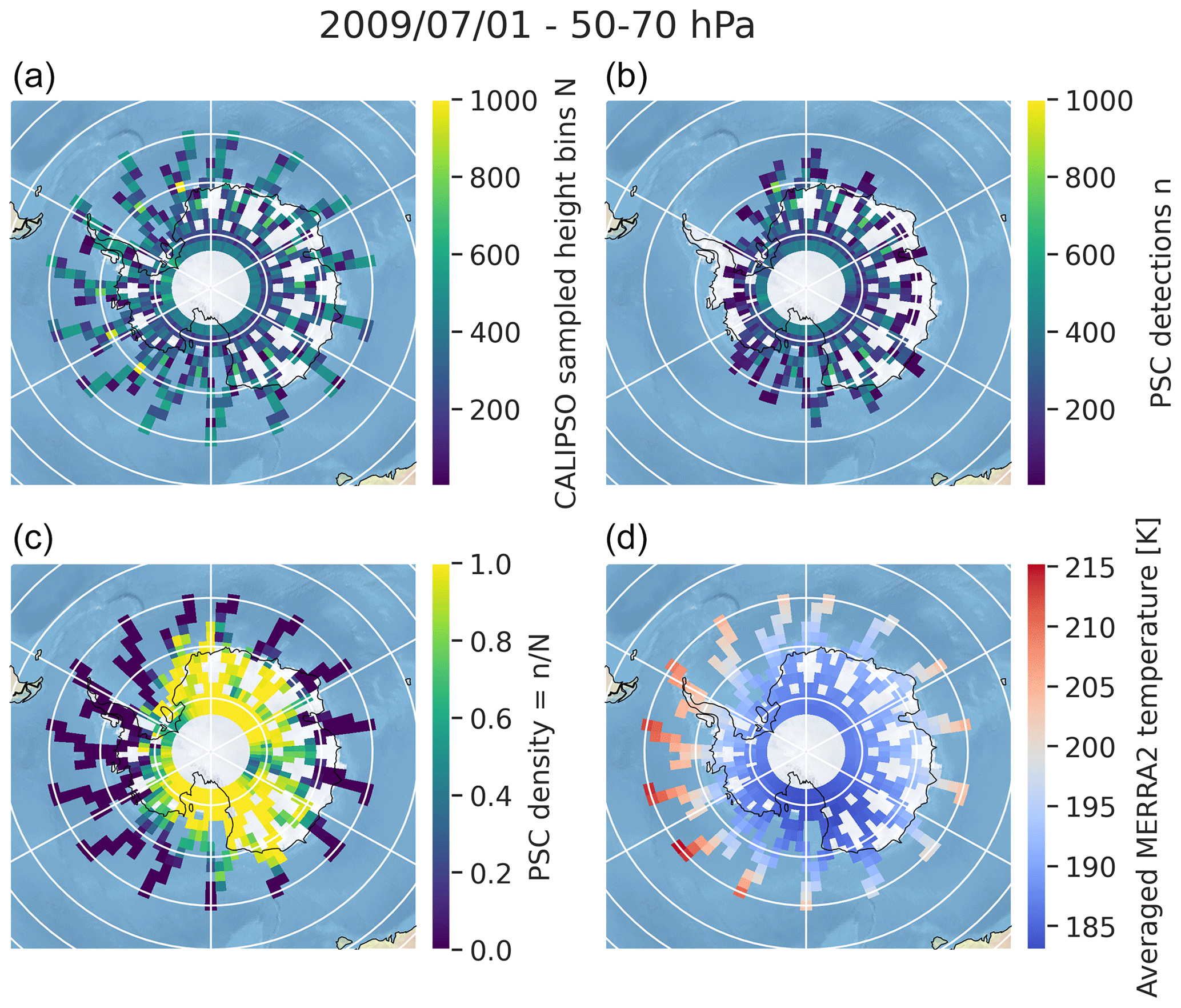
Figure 1 Output of daily gridding for 1 July 2009 between 50 and 70 hPa. (a) Number of sampled points N. (b) Number of PSC detections n. (c) PSC density F_lat,long(P) and (d) mean stratospheric temperature 〈T_lat,long〉 from MERRA-2.

Still for day d, we spatially average the daily gridded map of PSC density F_lat,long(P) for the level P (Fig. 1c) over the entire region to obtain a mean daily PSC density $\stackrel{\mathrm{‾}}{F_{\mathrm{d}}\left(P\right)}=\frac{\mathrm{1}}{\text{Nb}}{\sum }_{\mathrm{lat},\mathrm{long}}{F}_{\mathrm{lat},\mathrm{long}}\left(P\right)\cdot w$, with Nb the number of lat–long grid boxes sampled by CALIPSO and w the weight as a function of latitude, to take into account the zonal variation in grid box size. In parallel, in each lat–long grid box at the same level P we check if the temperature 〈T_lat,long〉 (Fig. 1d) is colder than a threshold T_psc (Fig. 2) to derive a map of cold density. The way T_psc is selected is described in Sect. 3.2. From the resulting map filled with 1 and 0 depending on whether the condition is met or not, we calculate a daily cold density $\stackrel{\mathrm{‾}}{C_{\mathrm{d}}\left(P\right)}=\frac{\mathrm{1}}{\text{Nb}}{\sum }_{\mathrm{lat},\mathrm{long}}x\cdot w$ with x = 1, where $\langle T_{\mathrm{lat},\mathrm{long}}\rangle <T_{\mathrm{psc}}$, Nb is the number of lat–long grid boxes sampled by CALIPSO, and w is the weight as a function of latitude. The daily $\stackrel{\mathrm{‾}}{F_{\mathrm{d}}\left(P\right)}$ and $\stackrel{\mathrm{‾}}{C_{\mathrm{d}}\left(P\right)}$ sum up the maps of Fig. 1c and d as a couple of single numbers for the entire polar region at a pressure level P. These values provide a convenient way to describe the extent of the PSC spatial cover on a given day, enabling the study of PSC evolution over long periods.

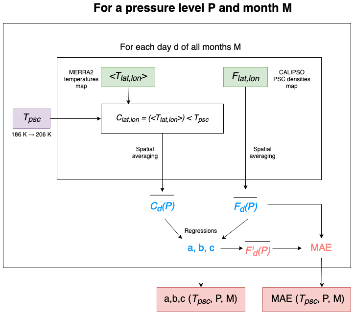
Figure 2 Flowchart describing the methodology. Green rectangles are input variables; in purple are the temperature thresholds which vary and in red the output parameters.

We follow the steps above to get ($\stackrel{\mathrm{‾}}{F_{\mathrm{d}}\left(P\right)}$, $\stackrel{\mathrm{‾}}{C_{\mathrm{d}}\left(P\right)})$ for each pressure level P and day of the PSC dataset. Then, we establish a relationship between these parameters for each pressure level P and month M of the PSC season (May to October, blue text in Fig. 2). Figure 3 shows an example of this process considering the 50–70 hPa pressure level. One point in these plots sums up daily maps like in Fig. 1. There are 465 or 450 points in each scatter plot, corresponding to the 31 or 30 d in each month from 2006 to 2020. Tests have shown that the lowest-order regression that provides the best fit for most of the plots is a polynomial fit of degree 2 (red lines, Fig. 3). The regression takes the form $\stackrel{\mathrm{‾}}{F_{\mathrm{d}}\left(P\right)}=a\cdot {\stackrel{\mathrm{‾}}{C_{\mathrm{d}}\left(P\right)}}^{\mathrm{2}}+b\cdot \stackrel{\mathrm{‾}}{C_{\mathrm{d}}\left(P\right)}+c$. These equations relate $\stackrel{\mathrm{‾}}{F_{\mathrm{d}}\left(P\right)}$ and $\stackrel{\mathrm{‾}}{C_{\mathrm{d}}\left(P\right)}$ for each pressure level P during each month of the PSC season and constitute our PSC model. They allow us to produce a mean estimated PSC density called $\stackrel{\mathrm{‾}}{F_{\mathrm{d}}^{\prime }\left(P\right)}$ from a known mean cold density $\stackrel{\mathrm{‾}}{C_{\mathrm{d}}\left(P\right)}$. This methodology is repeated for each month of the PSC season. In the next subsection, we explain the process of selecting T_psc and its significance in our analysis.

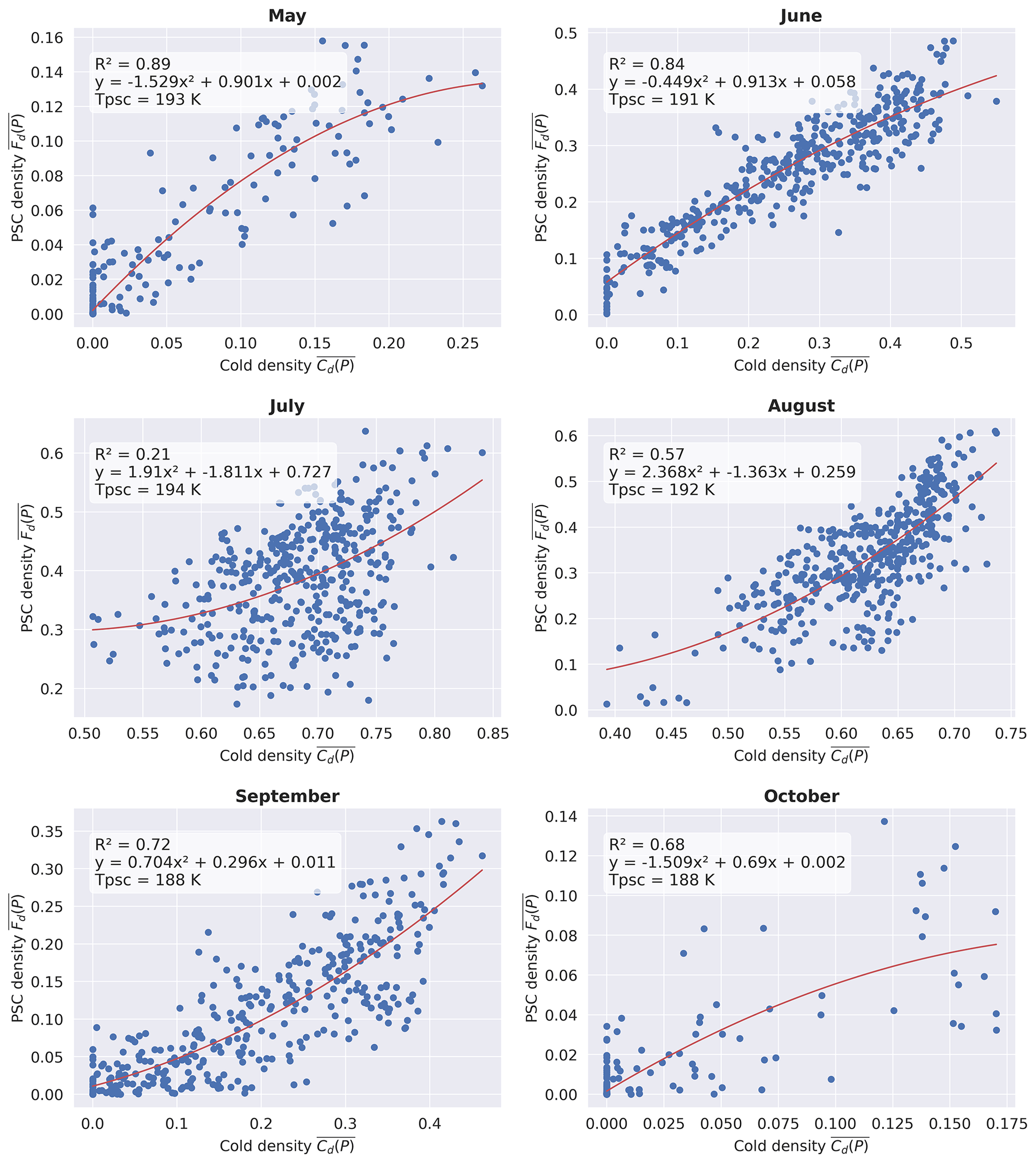
Figure 3 Monthly scatter plots for the 50–70 hPa pressure level over 2006–2020. Red lines are the trends, with their equations in white inset panels along with the correlation coefficients R² and T_psc.

3.2 Determination of T_psc

The selection of the temperature threshold T_psc is a crucial step. It is the temperature above which PSCs are not detected in the CALIPSO PSC product and above which our model will not predict PSC presence in a grid box. Here, we select T_psc as the temperature threshold that optimizes the agreement between the mean PSC density $\stackrel{\mathrm{‾}}{F_{\mathrm{d}}\left(P\right)}$ observed by CALIOP and the estimated mean PSC density $\stackrel{\mathrm{‾}}{F_{\mathrm{d}}^{\prime }\left(P\right)}$ generated by our model over the entire time period considered. In addition to cold temperatures, PSC formation requires appropriate concentrations of chemical species like HNO₃ and H₂O. These concentrations are not constant temporally or spatially, which is why we calculate a different T_psc for each pressure level and each month.

To find the optimal T_psc, for each pressure level P and each month M, we consider candidate temperature thresholds T_psc from 186 to 206 K. For each candidate T_psc, we calculate the mean cold density $\stackrel{\mathrm{‾}}{C_{\mathrm{d}}\left(P\right)}$ and conduct a polynomial regression between $\stackrel{\mathrm{‾}}{C_{\mathrm{d}}\left(P\right)}$ and $\stackrel{\mathrm{‾}}{F_{\mathrm{d}}\left(P\right)}$ (blue text in Fig. 2), which lets us estimate $\stackrel{\mathrm{‾}}{F_{\mathrm{d}}^{\prime }\left(P\right)}$. We then calculate between $\stackrel{\mathrm{‾}}{F_{\mathrm{d}}\left(P\right)}$ and $\stackrel{\mathrm{‾}}{F_{\mathrm{d}}^{\prime }\left(P\right)}$ the mean absolute error (MAE) (red text in Fig. 2), which quantifies the quality of the regression. The T_psc and regression parameters which lead to the smallest MAE are selected for the month and pressure level considered. MAE minima are well-defined enough to specify a T_psc with a precision of 1–2 K.

Below we compare the retrieved T_psc with the temperature of nitric acid nucleation T_NAT, which is the warmest temperature at which PSC particles can in theory start to form and subsist, considering all available chemical species (Tritscher at al., 2021). Using the formula of Hanson and Mauersberger (1988), we calculate T_NAT from the profiles of stratospheric temperature and of mixing ratio for HNO₃ and H₂O reported in the PSC product over separate pressure levels. For each daily file in the PSC product, we extracted HNO₃ and H₂O mixing ratios between 10 and 250 hPa and interpolated the H₂O mixing ratios on HNO₃ pressure levels. We calculated daily T_NAT from the mixing ratios and temperature at each pressure level. We interpolated T_NAT on the 121 altitude levels of the CALIPSO PSC product. As in Sect. 3.1, we averaged the T_NAT in our 3D spatial grid (latitude × longitude × pressure) and calculated the latitude-weighted spatial average to obtain a mean daily T_NAT vertical profile. Finally, we averaged these daily profiles to get an average T_NAT vertical profile for a given time period.

The T_NAT vertical profiles we calculated over the 2006–2020 period (Fig. 4) are consistent with the literature: at 14 km altitude (100 hPa), typical stratospheric mixing ratios are around 3 ppm for H₂O and 5 ppb for HNO₃, resulting in a T_NAT value of about 197 K (Hanson and Mauersberger, 1988), similar to our results. At 50 hPa, mixing ratios of 10 ppbv for HNO₃ and 5 ppmv for H₂O lead to a T_NAT value of about 195.7 K (Pitts et al., 2018), consistent with our result of 194 K. The T_psc vertical profiles we calculated over 2006–2020 are relatively close to the T_NAT profiles, especially in July. Both temperature thresholds T_NAT and T_psc become colder in the upper stratosphere and warmer at lower altitudes, except at 10–20 hPa for the September and October T_psc profiles. Apart from July, T_psc is generally significantly colder than T_NAT (more than several standard deviations apart). The difference is particularly important at lower altitudes between 30 and 100 hPa (Fig. 4, bottom left).

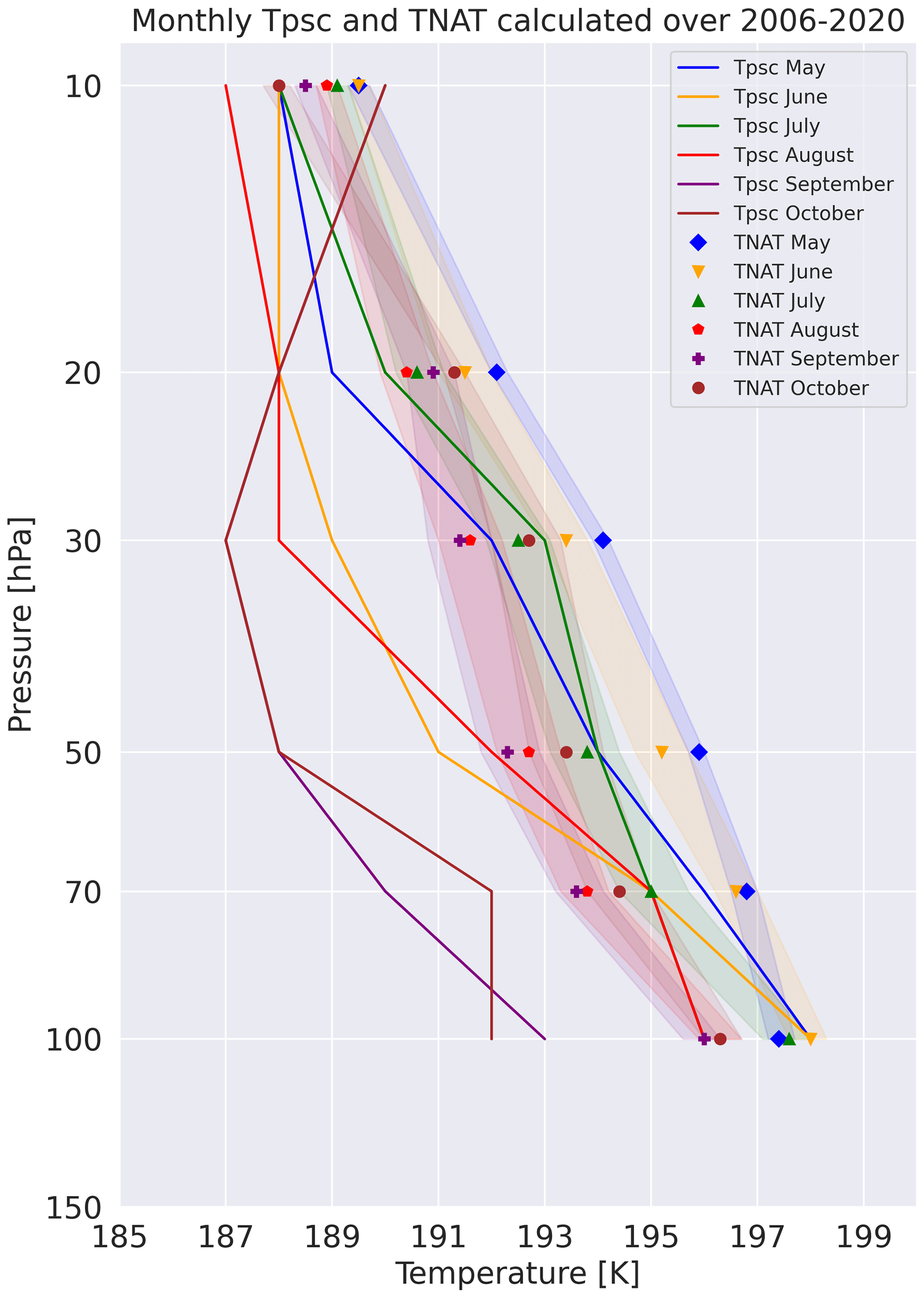
Figure 4 Vertical profiles of monthly T_psc (colored lines) and T_NAT (colored symbols). The colored envelopes represent the standard deviation of daily T_NAT.

PSC particles observed by CALIPSO in the lower stratosphere can come from nucleation processes when temperatures are below the threshold formation temperature T_NAT, but they can also be sedimenting from upper levels. The formation of PSC particles requires a long time in cold temperatures; thus, the mere occurrence of temperatures colder than T_NAT might not be sufficient for PSC detection in CALIPSO measurements. NAT particles may form but in concentrations too small to be detected. All these elements could explain why there is often a large difference between the temperature threshold T_NAT at which PSCs can form and the temperature threshold T_psc at which PSCs are observed. In the end, using T_psc significantly colder than T_NAT provides the best match between observed and predicted PSC densities.

3.3 Estimating PSC densities $\stackrel{\mathrm{‾}}{F_{\mathrm{d}}^{\prime }\left(P\right)}$

Once we have derived appropriate regression parameters and T_psc for each month M and pressure level P, we can use those to generate PSC densities $\stackrel{\mathrm{‾}}{F_{\mathrm{d}}^{\prime }\left(P\right)}$ on daily timescales across a specific period. To do so, for a given pressure level, we require a daily gridded map of temperature at large spatial scales. This map can be obtained either by regridding the temperatures profiles from the CALIPSO PSC product (as in Sect. 4) or straight from the MERRA-2 reanalysis dataset (as in Sect. 5). Considering the appropriate T_psc for the pressure level under study, from a daily map of temperatures we derive a daily average cold density $\stackrel{\mathrm{‾}}{C_{\mathrm{d}}\left(P\right)}$. We then apply the polynomial model (as in Sect. 3.1, Fig. 3) to the daily average cold density $\stackrel{\mathrm{‾}}{C_{\mathrm{d}}\left(P\right)}$ to output a daily average estimated PSC density $\stackrel{\mathrm{‾}}{F_{\mathrm{d}}^{\prime }\left(P\right)}$. Results for the 50–70 hPa pressure level of the estimated PSC densities $\stackrel{\mathrm{‾}}{F_{\mathrm{d}}^{\prime }\left(P\right)}$ derived from our model (Sect. 3.1) are shown in Appendix C.

4 Evolution of PSC densities over 14 years (2006–2020)

4.1 Model performance in estimating PSC densities

In this section, we compare the daily evolution of the observed PSC density $\stackrel{\mathrm{‾}}{F_{\mathrm{d}}\left(P\right)}$ (blue in Fig. 5, left column) with the estimated PSC density $\stackrel{\mathrm{‾}}{F_{\mathrm{d}}^{\prime }\left(P\right)}$ (red) generated by our model applied to MERRA-2 temperatures contained in the PSC product over the 2006–2020 period. PSC densities averaged (lines) over the whole period are well-reproduced by our model at all pressure levels. The MAE over the entire season between the average observed and estimated PSC densities is low overall but is slightly higher at lower levels from 0.003 (10–20 hPa) to 0.009 (100–150 hPa). Our model performance is the best in May, early June, and September–October: the discrepancies between average PSC densities observed and estimated are extremely low, and standard deviations from both our model and observations are similar. In those months, the maxima and minima are well-represented, especially between 50 and 150 hPa. At upper levels (10–20 and 20–30 hPa), even if some short-lived peaks in PSC densities are missed during the middle of the season, our model accurately captures the interannual variability and minima during the PSC season. Our model has a harder time estimating PSC density during the middle of the season, particularly in July and occasionally in August, resulting in a deteriorating MAE (0.01–0.02 on average). This is particularly visible at lower altitudes (50–70 and 70–100 hPa), where average PSC densities are sometimes overestimated or underestimated by our model, combined with a poorer interannual variability.

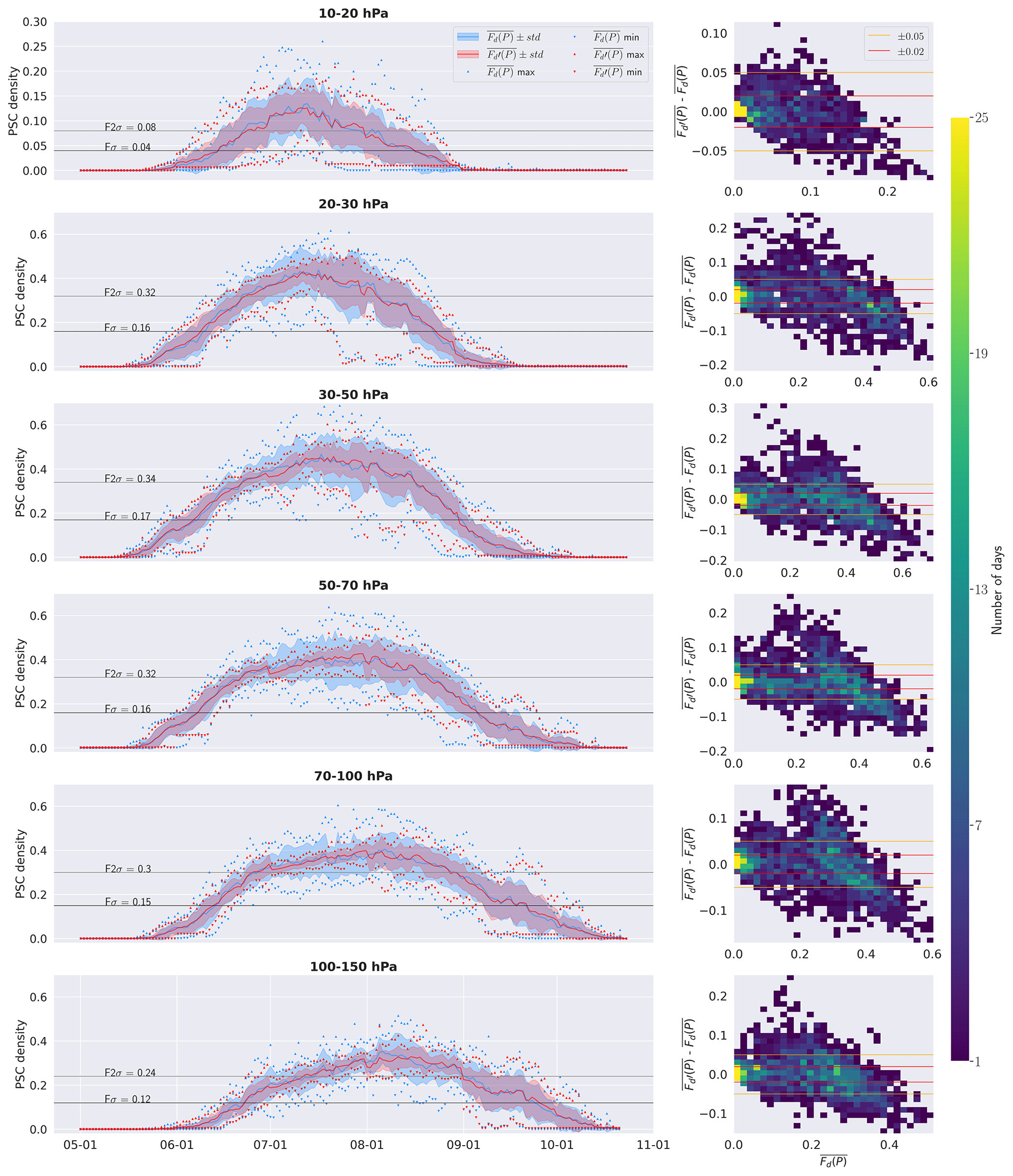
Figure 5 Left column: time series from 1 May to 31 October of the daily PSC density averaged over the 2006–2020 period (blue line for $\stackrel{\mathrm{‾}}{F_{\mathrm{d}}\left(P\right)}$, red line for $\stackrel{\mathrm{‾}}{F_{\mathrm{d}}^{\prime }\left(P\right)})$ with their standard deviation (blue and red envelopes) for each pressure level. Blue and red triangles represent the maximum and minimum daily densities. The black (gray) lines represent (twice) the mean standard deviations of the observed time series F_σ (F_2σ). Right column: 2D histogram of $\stackrel{\mathrm{‾}}{F_{\mathrm{d}}^{\prime }\left(P\right)}-\stackrel{\mathrm{‾}}{F_{\mathrm{d}}\left(P\right)}$ differences vs. $\stackrel{\mathrm{‾}}{F_{\mathrm{d}}\left(P\right)}$ for each pressure level.

At 10–20 hPa, the PSC densities are low compared to other pressure levels, and the daily differences between $\stackrel{\mathrm{‾}}{F_{\mathrm{d}}^{\prime }\left(P\right)}$ and $\stackrel{\mathrm{‾}}{F_{\mathrm{d}}\left(P\right)}$ are thus also low. For low observed PSC densities ($\stackrel{\mathrm{‾}}{F_{\mathrm{d}}\left(P\right)}<$ 0.1), although the error of our model can reach 0.05, with these values being less than 10 %, they remain negligible. For larger observed PSC densities ($\stackrel{\mathrm{‾}}{F_{\mathrm{d}}\left(P\right)}>$ 0.1), the daily differences can reach up to −0.1 (Fig. 5, right column). Finally, 80 % of simulated PSC densities are within ±0.02 (red lines) of retrievals, and 96 % are within ±0.05 (orange lines). Below 20 hPa, PSC densities are overall higher (0.4–0.5 at maximum) and more similar across pressure levels, resulting in a similar F_σ. Between 20 and 150 hPa, 50 % of estimated PSC densities are within ±0.02 of retrievals, and 74 % are within ±0.05. For low PSC densities ($\stackrel{\mathrm{‾}}{F_{\mathrm{d}}\left(P\right)}<$ 0.2), our model tends to overestimate the densities, with 20 % of the differences between $\stackrel{\mathrm{‾}}{F_{\mathrm{d}}\left(P\right)}$ and $\stackrel{\mathrm{‾}}{F_{\mathrm{d}}^{\prime }\left(P\right)}$ being above 0.02 vs. 10 % of the differences under −0.02. As observed PSC densities increase ($\stackrel{\mathrm{‾}}{F_{\mathrm{d}}\left(P\right)}>$ 0.2), our model tends to increasingly underestimate PSC densities in a linear way, with 47 % of the differences between $\stackrel{\mathrm{‾}}{F_{\mathrm{d}}\left(P\right)}$ and $\stackrel{\mathrm{‾}}{F_{\mathrm{d}}^{\prime }\left(P\right)}$ being under −0.02 vs. 29 % of differences above 0.02. These results suggest that our model manages to reproduce the distribution of daily PSC densities along the season over a long time period with appropriate accuracy.

4.2 Model performance in estimating PSC season start and end dates

We focus now on the start and end of the PSC season, according to observations and our model. For each pressure level, we mark the start of the PSC season when PSC densities first exceed F_σ the standard deviation of $\stackrel{\mathrm{‾}}{F_{\mathrm{d}}\left(P\right)}$ averaged over the 2006–2020 period (Fig. 5) and the end of the PSC season when PSC densities last dip below F_σ. In the rest of the paper, we define P_σ as the period when the PSC densities are larger than the standard deviation ($P_{\mathit{\sigma }}=\stackrel{\mathrm{‾}}{F_{\mathrm{d}}\left(P\right)}>F_{\mathit{\sigma }}$) and P_2σ as the period when PSC densities are larger than twice the standard deviation: $P_{\mathrm{2}\mathit{\sigma }}=\stackrel{\mathrm{‾}}{F_{\mathrm{d}}\left(P\right)}>F_{\mathrm{2}\mathit{\sigma }}$. PSC observations from 2006 were excluded from this part of the analysis since PSC data are not available before 13 June 2006.

Figure 6 shows the start and end dates of the PSC seasons for the 50–70 hPa pressure level, considering PSC densities from observations (lines) and from our model applied to temperatures from the CALIPSO PSC product (hatched regions). Overall, our model manages to estimate the PSC season start and end compared to observations with accuracy. At that pressure level on average over the 2007–2020 period our model and observations estimates the same start date and a quite similar end of the PSC season on 6 and 8 September, respectively (orange). Observations and the model agree that P_2σ starts on 22 June and ends on 20 August (blue). The largest disparity between observations and our model concerns the 2015 season, which our model ends 23 d late due to an overestimation of PSC densities (Appendix C).

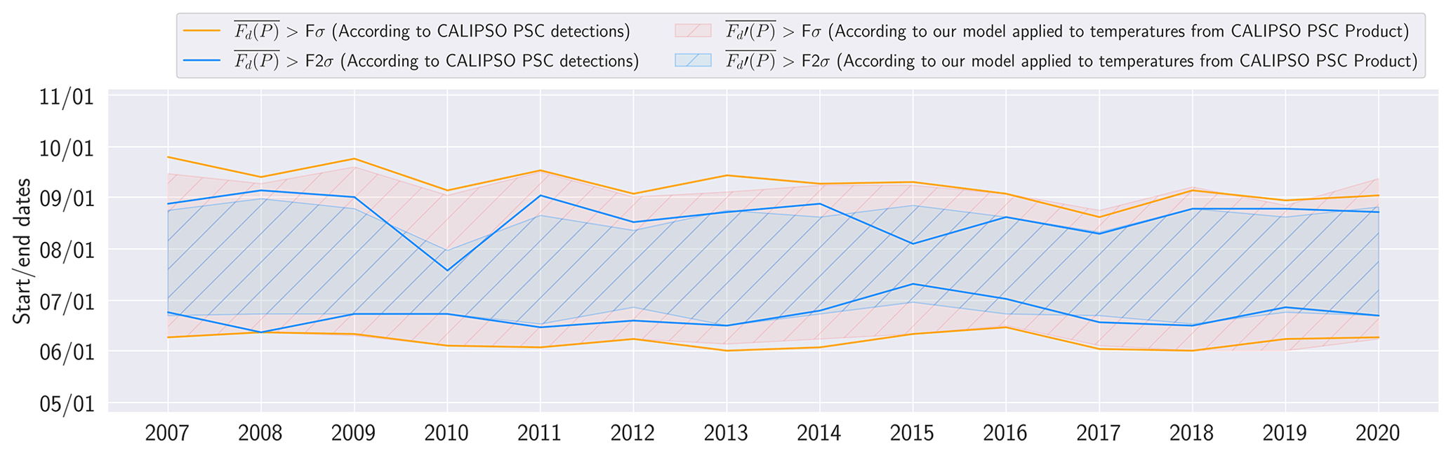
Figure 6 Start and end dates of P_σ (orange) and P_2σ (blue) for the 50–70 hPa pressure level for the time period 2007–2020. Full lines are based on PSC densities $\stackrel{\mathrm{‾}}{F_{\mathrm{d}}\left(P\right)}$ retrieved from CALIPSO PSC detections, and hatched surfaces are based on PSC densities $\stackrel{\mathrm{‾}}{F_{\mathrm{d}}^{\prime }\left(P\right)}$ derived from our model applied to MERRA-2 temperatures provided by the CALIPSO PSC product.

Looking at all pressure levels, our model and observations agree well on PSC season start and end dates, as differences never exceed 2–3 d (Fig. 7). Our model starts the PSC season (P_σ) slightly late (Fig. 7a), except at 20–30 and 70–100 hPa (red, Fig. 7a). The best performance of our model is between 10 and 100 hPa, with differences being on average less than a day with standard deviations between 3 and 4 d. The largest difference from observations is found at 100–150 hPa (2.6 ± 3 d) and remains small compared to the average length of seasons (months). Concerning the end of the PSC season (blue, Fig. 7a), our model puts it slightly too early except at 100–150 hPa. The average differences vary from 0 to 3 d with standard deviations between 5 and 10 d. Our model's most accurate estimation is at 70–100 hPa, with an average difference shorter than a day. Overall, the PSC season dates produced by our model and observed by CALIPSO agree extremely well within a few days at all pressure levels.

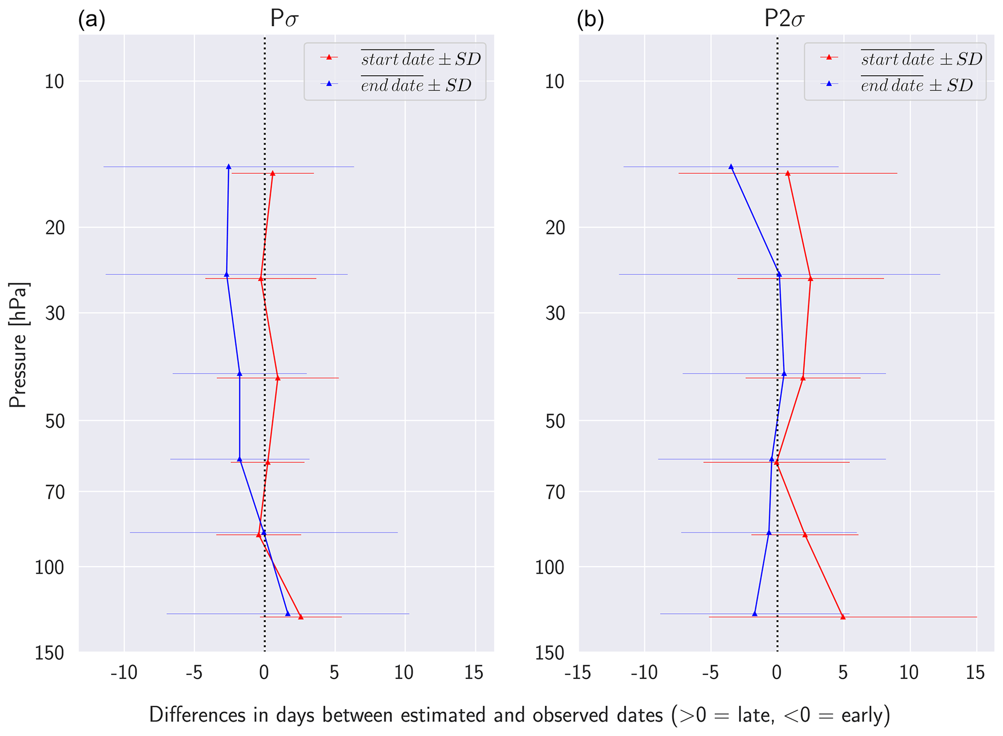
Figure 7 Vertical profiles of the average differences between the start (red) and end (blue) of P_σ (a) and P_2σ (b) periods according to CALIPSO observations and our model estimations over the 2007–2020 period. Our model is applied to MERRA-2 temperatures provided by the CALIPSO PSC product. The horizontal bars represent the standard deviations of differences.

Our model and observations generally start the P_2σ period within 2 d of each other on average (red, Fig. 7b), with the best agreement at 50–70 hPa. Standard deviations for the differences in start dates range between 4 and 10 d. Like with P_σ, we find the worst agreement for P_2σ at 100–150 hPa (with an average difference of 4.9 ± 10 d). The agreement for end dates is generally very good (blue in Fig. 7b), with differences below 3.5 d and standard deviations between 7 and 12 d. We find that end dates agree best between 20 and 100 hPa (< 1 d on average). While P_2σ estimation start dates are slightly less accurate than P_σ, they remain robust overall. However, P_2σ estimation end dates are more accurate than P_σ.

In summary, the boundaries of the P_σ and P_2σ periods derived from our model and observations agree extremely well, especially at 50–70 hPa. In general, our model tends to slightly shorten both periods due to a late start and an early end. Differences remain below 2–5 d, i.e., small relative to the typical season duration (months). As PSC seasons provided by our model appear to be consistent with the one derived from observations over the period 2007–2020, in the next section we extend our analysis into the past using MERRA-2 gridded temperatures over the 1980–2021 period.

5 Changes of the PSC season length over the 1980–2021 period

In this section, we investigate long-term changes in the length of the PSC season over the entire polar region (60–90° S) and over the CALIPSO sampling region (60–82° S) during the 1980–2021 period. To do so, we estimate daily PSC densities $\stackrel{\mathrm{‾}}{F_{\mathrm{d}}^{\prime }\left(P\right)}$ using MERRA-2 gridded temperatures, which cover the entire Antarctic region homogeneously every day. We assume that the PSC–temperature relationship we derived between 60 and 82° S is still valid south of 82° S. Since our model is built on the relationship between PSC detections from CALIPSO and MERRA-2 temperatures at large spatial resolutions, it is directly applicable to gridded temperatures from the same dataset. Compared to using temperatures from the CALIPSO PSC product, which sample different parts of the polar region every day, this approach leads to a more complete representation of daily PSC densities that does not suffer from sampling degradation due to variations in instrument operation or incoming sunlight.

5.1 PSC season duration

Over 1980–2021, between 60 and 90° S, the PSC season typically starts in early June, except between 20 and 50 hPa, where it starts in late May (Table 1 and red line in Fig. 8). The start dates of PSC season are quite stable, with standard deviations going from 4 d (50–100 hPa) to 9 d. Start dates appear relatively stable with pressure. A clear trend appears for end dates with increasingly later dates as we descend in altitude (blue line), going from 19 August at 10–20 hPa to 7 October at 100–150 hPa. Moreover, compared to start dates, end dates appear more variable, with standard deviations going from 6 d at 20–30 hPa to 13 d at 70–100 hPa. At lower altitudes, the PSC season begins later and finishes later, explaining why the PSC season last 1 to 2 months longer at lower altitudes.

Table 1 Average start and end dates of the PSC season over 1980–2021, the average length of the P_σ season, and the changes in the PSC season duration according to linear regressions for each pressure level and over the two latitudinal regions of 60–90 and 60–82° S.

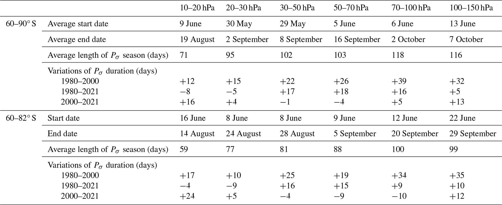
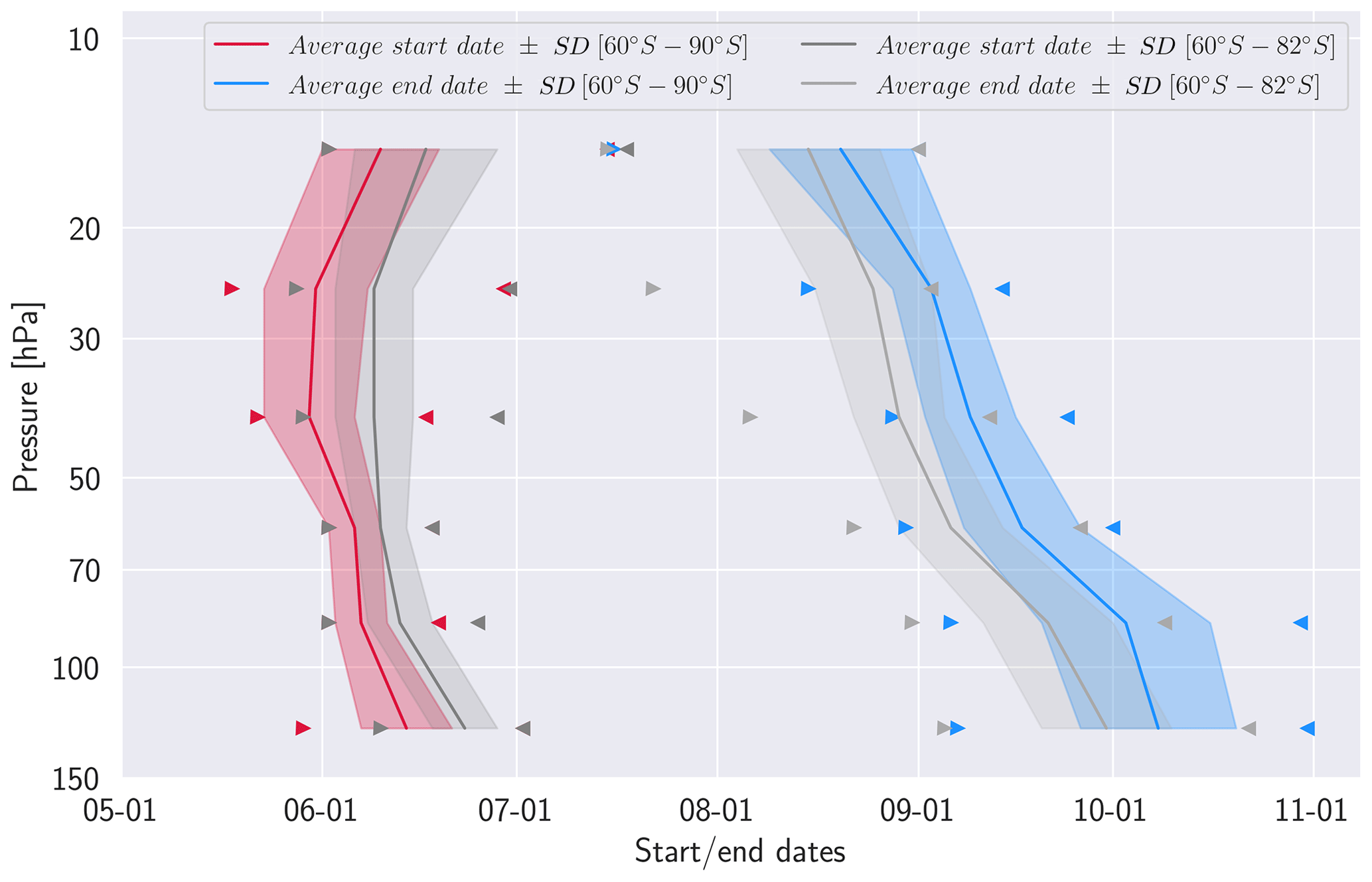
Figure 8 Start (pink) and end (blue) of the PSC season averaged over 1980–2021 across pressure levels. Colored lines are over the entire polar region (60–90° S), and gray lines are over the CALIPSO sampling region (60–82° S). Triangles represent the earliest start and end dates over the 1980–2021 period. Envelopes represent the standard deviations.

Between 60 and 82° S, the PSC season typically starts in June and begins approximately 4 to 11 d later than when considering the entire polar region. End dates are less spread than between 60 and 90° S, from 14 August at 10 hPa to 29 September at 150 hPa. Differences are largest at 30–50 hPa, where there is an 11 d gap. Between 60 and 82° S, the PSC season presents a later onset as well as an earlier end, and by consequence seasons are shorter (Appendix D). These results suggests that as CALIPSO does not sample the region poleward of 82° S, it misses early PSC close to the pole and late PSCs that persist there towards the end of the season. At 10–20 hPa, the season begins more than 1 week later for 14 years and more than 2 weeks later for 5 years compared to the period considered across the entire polar region. ln 1982 and 2010, the start of the PSC season is delayed by 26 d, and in 2006, it is delayed by 35 d. For other pressure levels, the PSC season starts between 1 and 2 weeks later than between 60 and 90° S. The pressure level least impacted by the latitudinal region is at 50–70 hPa, where it shows minimal start date differences, with only 4 years beginning more than 1 week later. Most of the time, the gap remains less than a week and is very often zero. This result suggests that PSCs form first between 82 and 60° S each year at 50–70 hPa. For end dates, when comparing the 60–82 and the 60–90° S regions, the greatest differences appear between 30 and 100 hPa, with on average 29 years ending more than 1 week earlier and 12 years ending more than 2 weeks earlier. The largest gap is at 70–100 hPa, with 2 years ending 32 and 36 d earlier.

5.2 Changes in PSC season duration

Here, we describe the evolution of the PSC season length according to trends retrieved over several decades (1980–2021). Over each pressure level, we examine the time series describing the annual duration of the PSC season (Appendix D), and on this time series we conduct a linear regression to retrieve the slope of the trend in PSC season length vs. time. From these regressions we estimate a change in PSC season length over long periods. Statistical tests on the estimated slope coefficients (Seabold and Perktold, 2010) are used to establish if the retrieved trends are statistically significant (p value < 0.05). We look independently at periods before and after 2000, as we found them to exhibit different behaviors.

Over the 1980–2000 period (Fig. 9a), we find that the PSC seasons get significantly longer (red lines, Fig. 9a). The increase exceeds the standard deviation of the series (dark green) at all pressure levels. Increases in PSC season length get longer at lower altitudes – they exceed twice the standard deviation (light green) and are found to be statistically significant (30–150 hPa). We find the PSC season increases the most at 70–100 hPa (+39 d between 60 and 90° S, +34 d between 60 and 82° S). We note that over the 1980–2000 period, MERRA-2 stratospheric temperatures exhibit substantial biases in the polar southern hemisphere (Lawrence et al., 2018), notably a warm bias (up to +1.5 K) at 30–70 hPa and a cold bias (−1 K) at 70–150 hPa. These biases could impact the length of the PSC season retrieved through our model, but as they remained constant over the 1980–2000 period, trends should not be affected. Between 10 and 30 hPa, MERRA-2 shows a cold bias over the 1980–2000 period, which increases to reach −3 K between 1994 and 1999. This bias could lead us to overestimate the length of PSC season at the end of the 1980–2000 period and overestimate the increasing trend. At those levels, however, the trends we retrieve are the weakest ones.

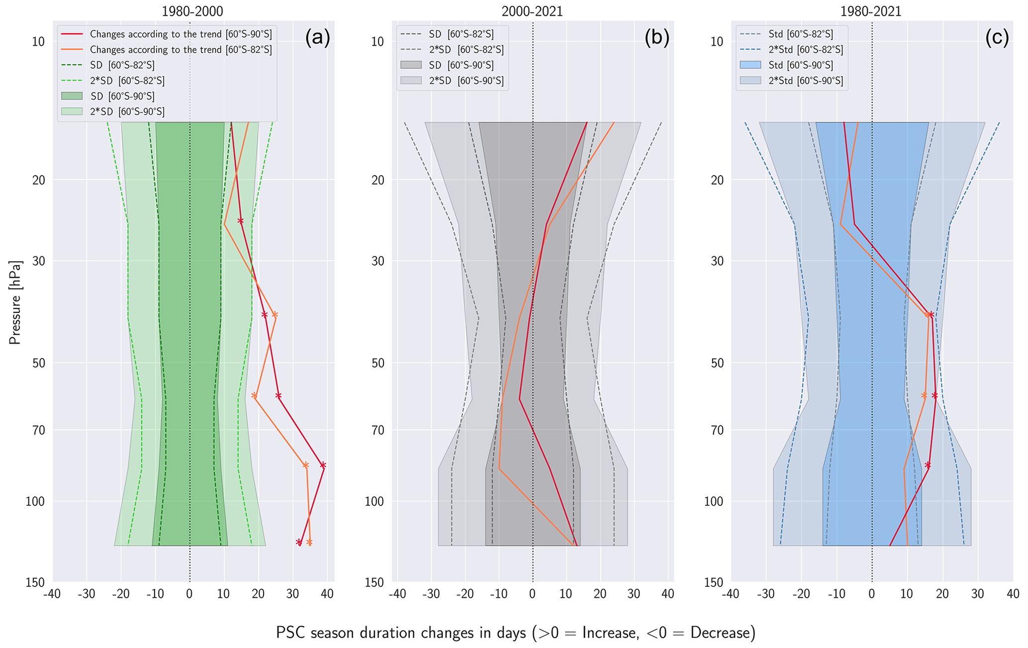
Figure 9 PSC season duration changes between 1980 and 2000 (a), between 2000 and 2021 (b), and between 1980 and 2021 (c) for each pressure level over the polar region (60–90° S) and over the CALIPSO sampling region (60–82° S) derived from trend analyses using from linear regressions. The red (pink) lines represent the changes in the number of days of the PSC season duration in the 60–90° S (60–82° S) region. The envelopes represent the standard deviations associated with the time series of the PSC season duration. The stars indicate significant trends.

Over the 2000–2021 period (Fig. 9b), we find no significant trend. This is explained by the small change in PSC season length according to regressions (less than 10 d between 20 and 100 hPa, red lines) combined with the enhanced variability of the PSC season length (gray shading) due to sudden stratospheric warming (SSW) events (e.g., 2002, 2019, Sect. 6) and warmer polar vortex occurrences (e.g., 2010, 2012). The PSC season tends to get shorter between 30 and 70 hPa over 60–90° S and between 30 and 100 hPa over 60–82° S. This result is in agreement with CALIPSO observations, which observed a statistically significant decrease in the PSC season length at 50–70 and 70–100 hPa (Appendix D). We note that at 70–100 hPa, the sign of the trend depends on the region: across the entire polar region the PSC season extends by 5 d, while it is shortened by 10 d over the CALIPSO sampling region. This result suggests that due to their incomplete spatial and temporal sampling CALIPSO observations are not always representative of long-term trends in the variability of the PSC cover across the entire polar region.

Over the 1980–2021 period (Fig. 9c), changes in PSC season lengths (red lines) are modest and often stay below a single standard deviation (blue shade). We find, however, a statistically significant increase between 30 and 100 hPa of up to +18 d at 50–70 hPa, twice the standard deviation. As discussed before, until 1999 MERRA-2 exhibits a substantial warm bias between 30 and 70 hPa, which disappears at once afterwards. This bias could lead to a sudden drop in MERRA-2 temperatures and an increase in PSC season duration as retrieved from our model. When examining the PSC season length (Appendix D), we find no sudden increase in PSC season length after 1999, suggesting that MERRA-2 biases do not substantially impact our results. At upper levels (10–30 hPa), the PSC season gets shorter over the 1980–2021 period, while it appeared to get longer over both the 1980–2000 and the 2000–2021 periods. We relate those trends to the 1999 disappearance of the strong cold bias in MERRA-2 temperatures at those levels, leading to a shortening of the PSC seasons.

6 Influence of synoptic events affecting the stratosphere

Large-scale atmospheric waves moving upwards into the stratosphere can disrupt the polar vortex. In extreme cases, this disruption triggers a reversal of wind directions and a rapid warming, known as a sudden stratospheric warming (e.g., SSW, Butler et al., 2015). In the Southern Hemisphere SSW events are rare, approximately one in 22 years (Jucker et al., 2021). The first SSW observed over the Antarctic was in 1988 with two warming events (Roy et al., 2022), the first a few days long and the second from 24 September to 3 October with a warming from 205 to 245 K. In our results, 1988 shows the earliest end of the PSC season at 50–70 hPa, and the early season ends between 70 and 150 hPa (Fig. 10). During the second SSW, in 2002, multiple wave events (Newman and Nash, 2005) led to a warming in June which became extremely intense by early July. We find at 50–70 hPa low PSC densities (< 0.2) in June compared to other years (not shown) and an early season end between 50 and 150 hPa. Combined with a late onset of the PSC season (early July), this led to a short PSC season (Fig. 10), the shortest at 100–150 hPa (78 d over 60–90° S and 69 d over 60–82° S, Appendix D) and 50–70 hPa over 60–82° S (68 d). During a third SSW in 2019 a strong planetary wave led to an exceptional rise in MERRA-2 temperature of +50.8 K at 10 hPa from 5 to 11 September (Yamazaki et al., 2020; Lim et al., 2021). By comparison, the maximum warming during September 2002 was 38.5 K per week. At 10–20 hPa, this warming did not impact our results since the PSC season was already over. Between 20 and 150 hPa, the PSC season end in early September due to the warming. Moreover, between 50 and 150 hPa, we notice a significant decrease in estimated PSC densities in late August (not shown), consistent with the SSW, leading to an early PSC end of season (Fig. 10). Based on these findings, we conclude that our model captures the impact that the SSW events have on PSC well, as long as their influence is correctly represented in the reanalyses. Other dynamic events that disturb the polar vortex appear equally well-captured by our model: for instance, in July 2010, a negative quasi-biennial oscillation favored the channeling of planetary waves, which produced a warming at high altitudes, especially at 10 hPa (Klekociuk et al., 2011). The related intense July warming leads to the earliest end of the PSC season at 10–20 hPa (Fig. 10).

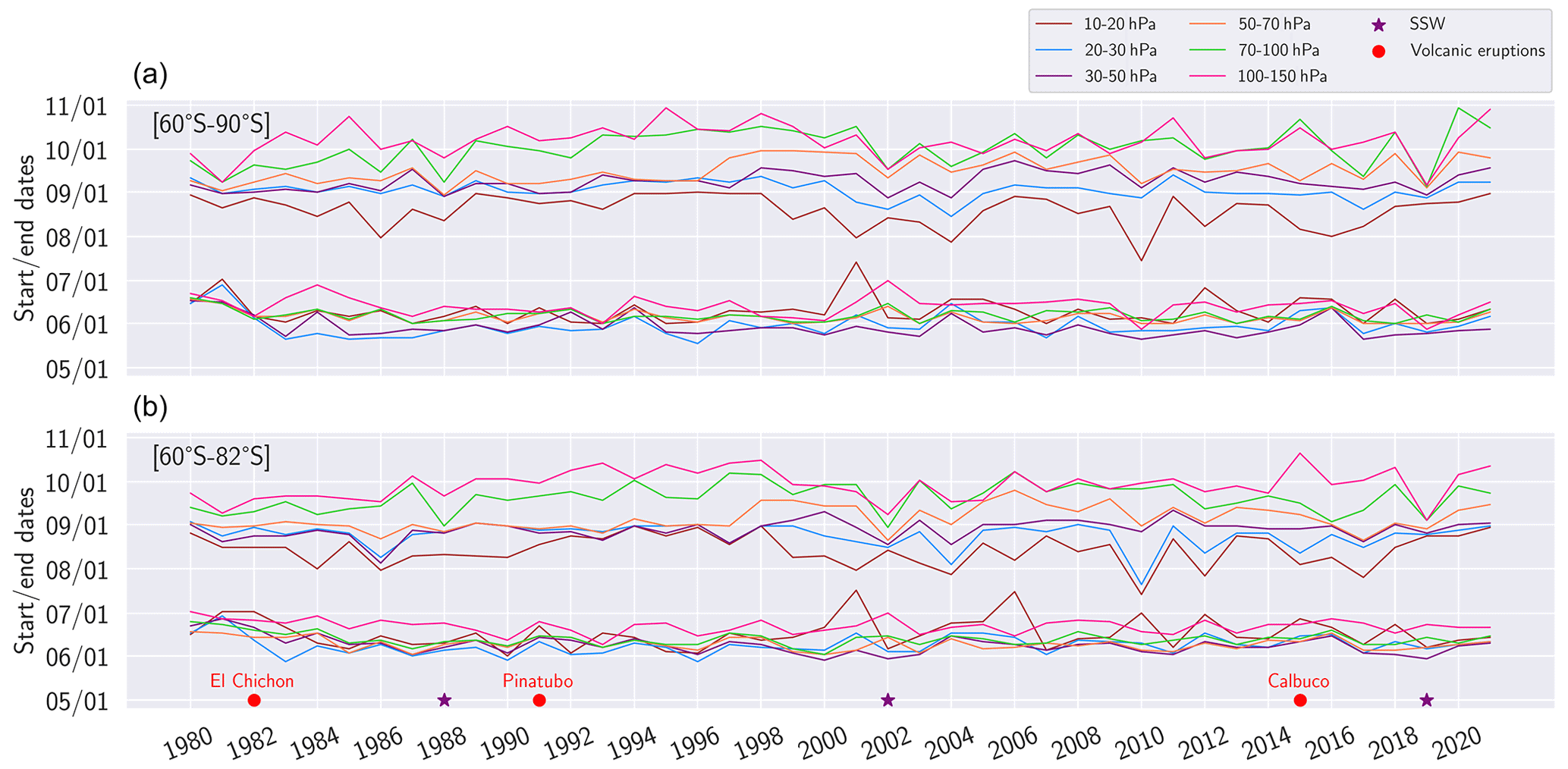
Figure 10 (a) Start and end of PSC seasons for each year between 1980 and 2021 over (a) the entire polar region (60–90° S) and (b) the CALIPSO sampling region (60–82° S). The red points represent volcanic eruptions and purple stars SSWs.

In addition to SSW, the polar stratosphere can be affected by volcanic events. The eruption of Mount Calbuco in April 2015, injected water and sulfate aerosols into the stratosphere, which slowly descended during transport from midlatitudes towards the poles (Stone et al., 2017). These injections began penetrating the Antarctic vortex in May, causing strong early denitrification and thus limiting PSC formation for the rest of the season (Zhu et al., 2018). CALIOP observations at the end of May reveal high PSC densities at 50–70 hPa compared to other years (Appendix C). This early surge in PSC densities is mostly due to NAT PSC (Appendix E) and is followed by a decline in early June, providing confirmation of early denitrification. Moreover, between 50 and 150 hPa, we found low STS and NAT densities (< 0.2) during the middle of the season, unlike other years where densities are twice as high. The absence of high PSC STS and NAT densities in this period suggests there is no longer enough HNO₃ and H₂O available in the stratosphere due to the early denitrification. Moreover, our temperature-based model overestimates the observed PSC densities between 50 and 100 hPa in July and August. The aerosols injected by volcanic eruptions capture some of the solar radiation, warming the atmosphere near their height of injection but cooling the lower altitudes. MERRA-2 temperatures at 50–70 and 100–150 hPa show a cold anomaly (Appendix E) compared to the 1980–2021 mean temperature from mid-July toward October, probably due to the cooling effect of the sulfate aerosols. Also notable is the prolonged 2015 PSC season at 100–150 hPa according to CALIPSO observations, showing uncommon high densities (∼ 0.2) in early October when PSC densities are in general below 0.1. Our model underestimates these high PSC densities, suggesting that factors beyond temperature influence the PSC formation, such as the aerosol supply resulting from the eruption. Overall, when considering CALIPSO PSC detections, volcanic eruptions appear to have a much weaker impact on the length of the PSC season than SSWs.

While our model can react to volcanic eruptions when their radiative effects are accounted for in the stratospheric temperatures, it cannot take into account their impacts on stratospheric polar chemistry. Such changes will depend on the volcano location and distance to the poles, on the eruption intensity and position within the season timeline, and on which chemical compounds are released by the eruption to reach the polar stratosphere. For example, the Hunga Tonga-Hunga Ha'apai eruption in 2022 injected huge amounts of water vapor into the stratosphere, but these did not penetrate the polar vortex: satellite measurements revealed that within the vortex, water vapor, ozone, and other chemical species maintained levels close to historical averages through spring 2022 (Manney et al., 2023). Complications with the calibration of the CALIPSO signal in the stratosphere affected by Hunga Tonga explains why the PSC product is not available for the 2022 Antarctic winter and why we cannot yet conclude anything about the effect of this eruption on the PSC formation and season. Outside the CALIPSO period and inside the 1980–2021 period, other volcanic eruptions include El Chichón (17° N, 93° W) in 1982, as well as Mount Cerro Hudson (46° S, 73° W) and Mount Pinatubo (15° N, 120° E), both in 1991. The Pinatubo eruption between 12 and 16 June 1991 was the most significant in the past century, releasing sulfur dioxide (SO₂) into the stratosphere, which was transformed into sulfate aerosols (${\mathrm{H}}_{\mathrm{2}}{\mathrm{SO}}_{\mathrm{4}}/{\mathrm{H}}_{\mathrm{2}}\mathrm{O}$) (McCormick et al., 1995), mostly affecting the Southern Hemisphere. MERRA-2 shows an episodic temperature increase between 10 and 100 hPa associated with the eruptions cited above (Gelaro et al., 2017). The cooling of the global mean stratosphere was more pronounced over the 1979–1998 period due to intense ozone depletion and increasing GHG emissions compared to the 1998–2016 period when ozone-depleting substances decreased (Maycock et al., 2018). Those results are consistent with the trends of the PSC season duration estimated by our model (Sect. 5). Indeed, our model finds that over 1980–2000 the PSC season gets longer at all pressure levels, consistent with a global cooling of the stratosphere. After 2000, the PSC season duration is stable, consistent with relatively warm years. To our knowledge, there is no evidence in the literature that confirms a PSC season extension over the 1980–2000 period. Merging retrievals from several satellites (Fromm et al., 2003) showed that PSCs were less frequent in July at 20 km a.s.l. in the Antarctic vortex in years characterized by volcanic eruptions, such as after the eruptions of El Chichón, Nevado del Ruiz, and Mount Pinatubo. Moreover, those years were characterized by a strong aerosol extinction inside the Antarctic vortex. These results suggest that in the case of major stratospheric eruptions, enhanced aerosol loading inside the polar vortex could trigger early denitrification and by consequence less PSC formation in the middle of the season, like for the Calbuco eruption in 2015. However, this does not imply a shortening of the PSC season, only lower PSC densities during the middle of the season.

7 Conclusions

In this article, we aimed to evaluate if the seasonal evolution of PSCs went through significant changes over the past decades (1980–2021). To reach this objective, we defined the daily PSC density as an indicator to track the fraction of the polar stratosphere covered by PSCs for pressure level ranges. By relating the PSC density to temperature data from MERRA-2, we developed a statistical model which estimates by pressure level the daily average PSC density over the polar region. We evaluated the robustness of our model by conducting comparisons between the observed PSC density data from CALIPSO and those estimated by our model.

The PSC–temperature relationship proposed by our model tracks the daily evolution of PSCs well throughout each season and at each pressure level between 10 and 150 hPa. Our model manages to reproduce the observed evolution of PSC in the case of well-understood stratospheric temperature changes driven by SSW (e.g., 2019, Sect. 6). However, if radiative forcing by aerosols from eruptions is not accounted for in stratospheric temperatures, the PSC–temperature relationship can be disrupted and our model will deviate from reality. Moreover, variations in aerosols and chemical species abundance, following volcanic eruptions, can affect our model's performance (e.g., the Calbuco eruption in 2015) in hard-to-predict ways due to the complex nature of their impact on PSC formation. Nevertheless, temperature generally appears to be a robust proxy for PSC formation at daily scales in most seasons, which enables a realistic capture of long-term changes. After defining the beginning and end of each PSC season based on variations of the PSC density, we found the results of our model to be in very good agreement with observations, with an accuracy better than 5 d at all pressure levels.

Applying our model to gridded MERRA-2 temperatures enabled us to quantify the PSC density (1) considering the whole Antarctica domain (2) at daily scales and (3) over the 1980–2021 period. This leads to an integrated view of PSC occurrence that is free from the sampling issues that spaceborne measurements can incur. Analyzing this dataset shows that the length of the estimated PSC season duration is systematically longer when considering the entire polar region than only the CALIPSO sampling region. We find that the PSC season gets significantly longer during the 1980–2000 period across all levels except at 10–20 hPa, with the largest increase (+39 d) at 70–100 hPa. The lengthening of the PSC season at upper levels (10–30 hPa) must be considered with caution due to the increasing cold bias in MERRA-2 temperatures between 1980 and 2000. However, all the significant trends found between 30 and 150 hPa are reliable even considering MERRA-2 biases. At high altitudes, the increasing PSC season length is attributed to an earlier start date and a later end date, while at other pressure levels, the lengthening of the season is due to later end dates only. After 2000, MERRA-2 temperature bias are reduced to become insignificant, inducing a drop in the PSC season length at 10–20, 20–30, and 100–150 hPa. Between 30 and 70 hPa, the PSC season tends to be slightly shortened; however, those trends are not significant. Over the 1980–2021 period, between 30 and 100 hPa, the PSC season gets significantly longer by 17 d on average. This lengthening is linked to a period of general stratospheric cooling. However, due to the bias present at all pressure levels in MERRA-2 before 1999, the trends found over the 1980–2021 period should be considered with caution.

Since our study associates observed PSC cover with MERRA-2 temperatures, applying our model to temperatures from other sources (e.g., ERA5 or climate models) would require re-training the model to account for baseline shifts in stratospheric temperatures for a particular dataset. Considering other reanalysis could help when examining the PSC season length, extracting MERRA-2 biases. According to Chap. 10 of the SPARC report, the best reanalysis with the lowest bias over the 1980–2021 period and all pressure levels seems to be JRA-55. Moreover, CALIPSO did not sample Antarctic regions south of 82° S, and variations in the PSC–temperature relationship in that region cannot be taken into account. There is, however, to our knowledge, no evidence for such variations. Finally, events of regional-scale gravity wave cooling, which might be underrepresented in reanalyses, can trigger PSC formation (Noel and Pitts, 2012). These PSCs, however, constitute a relatively small fraction of the overall PSC cover and their impact on the model's performance is considered negligible.

Future work may involve extending the scope of the present study to PSCs from the Arctic region, where stratospheric temperatures are less stable and PSC season durations more variable. First results suggest that our model can reproduce the PSC densities observed over the North Pole over the 2006–2020 period as well as over Antarctica. Adding PSC speciation to our model would enable the study of the evolution of a particular PSC type over long periods. Moreover, the gridded MERRA-2 temperatures are available four times a day, so we could document the PSC density evolution at sub-daily scales. Finally, we intend to apply our model to stratospheric temperatures predicted by general circulation models over the next century to better understand the evolution of PSC cover in the context of climate change and how it could impact the reformation of the hole in the ozone layer.

Appendix A: CALIPSO sampling

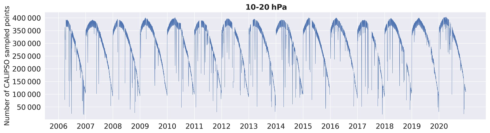
The total daily number of CALIPSO profiles over a PSC season (May to October) from 2006 to 2020 at 10–20 hPa exhibits a yearly pattern, which illustrates the deterioration of CALIPSO PSC sampling as the season ends due to the return of sunlight during austral spring. Low mid-season daily numbers of CALIPSO profiles can be related to CALIOP satellite maneuvers. In such cases, the payload is turned off, leading to irregular sampling and days excluded from the time series. In October, the daily number drops below 16 % of its maximum.

Figure A1 Total daily number of CALIPSO points from 2006 to 2020 at 10–20 hPa.

We sum up the percentage of available CALIPSO daily files from 2007 to 2020 below for each month of the PSC season (May to October).

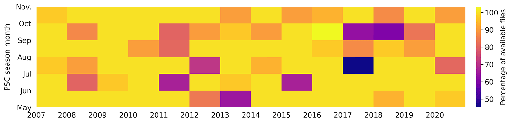
Figure A2 Percentage of available daily files for each month of the PSC season from 2007 to 2020.

Appendix B: Monthly temperature thresholds and statistical parameters (2006–2020)

Table B1 Monthly temperature thresholds T_psc by pressure level P and statistical parameters derived from comparisons between PSC densities observed by CALIPSO and those simulated by our model over the 2006–2020 period.

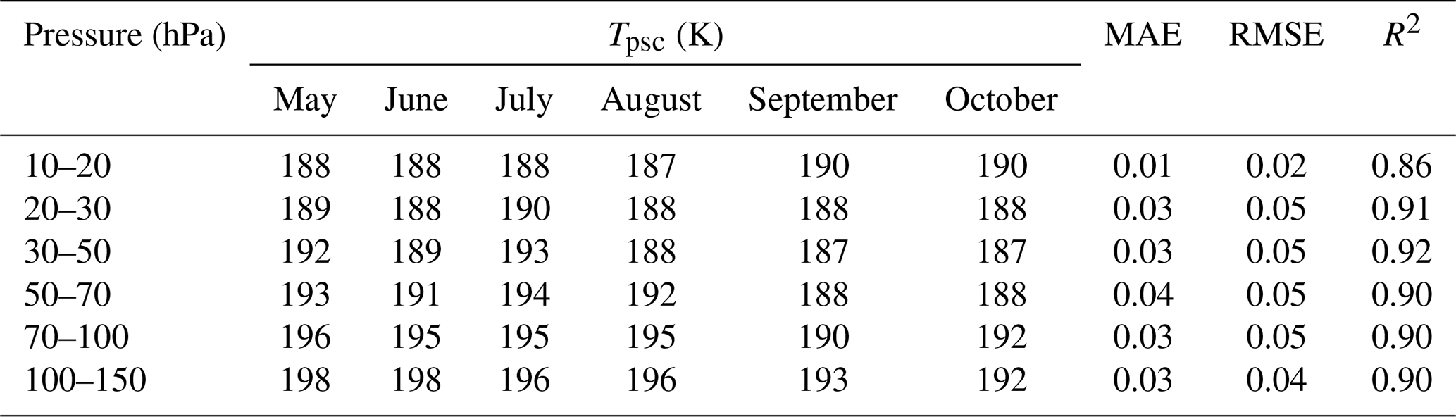
MAE (mean absolute error) is a measure of the prediction difference between two time series.

$$\begin{array}{rl}& \text{MAE}={\displaystyle \frac{{\sum }_{\mathrm{days}}\left|\stackrel{\mathrm{‾}}{F_{\mathrm{d}}\left(P\right)}-\stackrel{\mathrm{‾}}{F_{\mathrm{d}}^{\prime }\left(P\right)}\right|}{n}},\\ & \text{with}n\text{the number of days}\end{array}$$

RMSE (root mean square error) is a measure of the overall error between two time series. The lower the RMSE, the better the fit between the two series.

$$\begin{array}{rl}& \text{RMSE}=\sqrt{{\displaystyle \frac{{\sum }_{\mathrm{days}}{\left(\stackrel{\mathrm{‾}}{F_{\mathrm{d}}\left(P\right)}-\stackrel{\mathrm{‾}}{F_{\mathrm{d}}^{\prime }\left(P\right)}\right)}^{\mathrm{2}}}{n}}},\\ & \text{with}n\text{the number of days}\end{array}$$

R² (coefficient of determination) is a measure of the proportion of the variance of the reference series compared to the series to be evaluated. An R² of 1 indicates a perfect fit, while an R² of 0 indicates that there is no relationship between two series.

Appendix C: Estimated PSC densities by our model at 50–70 hPa

Figure C1 depicts, for the 50–70 hPa pressure level, the estimated PSC density $\stackrel{\mathrm{‾}}{F_{\mathrm{d}}^{\prime }\left(P\right)}$ compared to those observed by CALIPSO. Our model represents PSC densities well, except in July and August 2015 when $\stackrel{\mathrm{‾}}{F_{\mathrm{d}}^{\prime }\left(P\right)}$ values are larger than observations by up to 25 %. This year was characterized by the Calbuco eruption, which impacted stratospheric aerosol concentrations (Zhu et al., 2018). Such changes cannot be taken into account in our model, which is temperature-based.

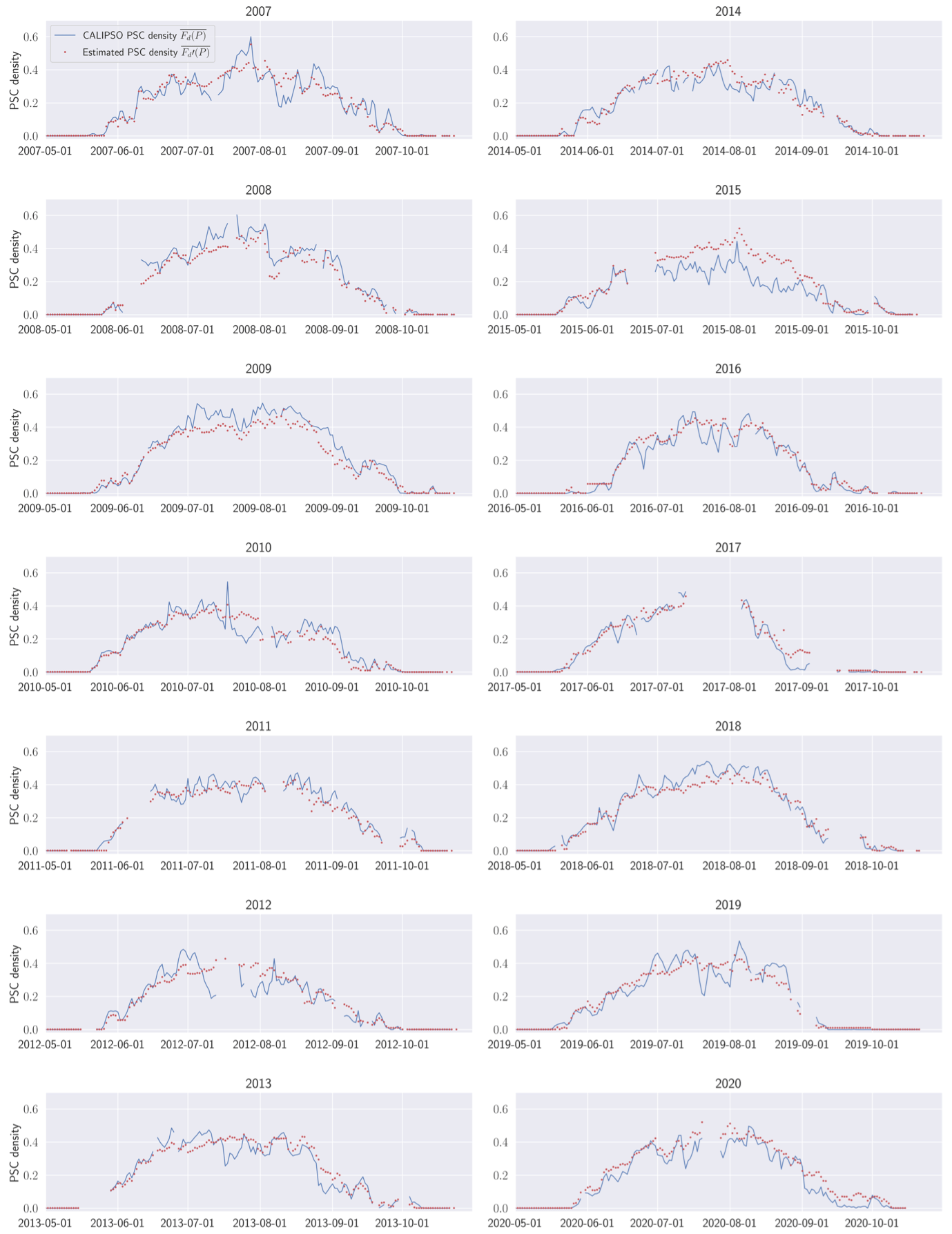
Figure C1 Time series from 1 May to 31 October of the daily PSC densities observed by CALIPSO $\stackrel{\mathrm{‾}}{F_{\mathrm{d}}\left(P\right)}$ (blue) and estimated by our model $\stackrel{\mathrm{‾}}{F_{\mathrm{d}}^{\prime }\left(P\right)}$ (red) from 2007 to 2020 at 50–70 hPa.

Appendix D: PSC season duration evolution over all pressure levels

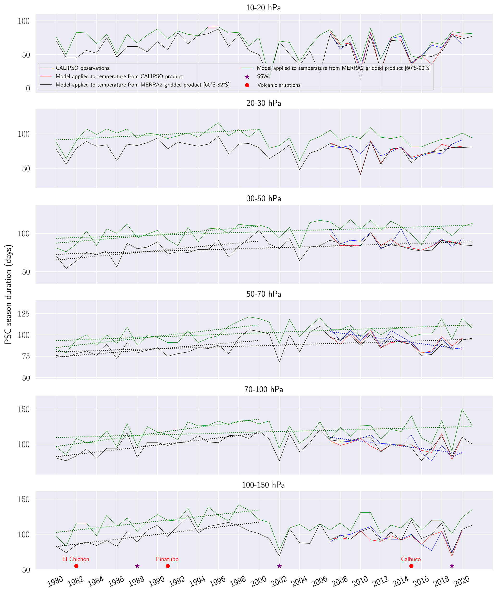
Figure D1 PSC season duration from 1980 to 2021 over all pressure levels according to our model applied to gridded MERRA-2 temperatures over 60–82° S (black) and over 60–90° S (green). In blue is the PSC season duration observed by CALIPSO and in red is that estimated by our model applied to temperatures provided by the CALIPSO PSC product. The red points represent the volcanic eruptions and purple stars the SSW. Only statistically significant trends are shown in dashed lines.

Appendix E: PSC density evolution and season changes at 50–70 hPa

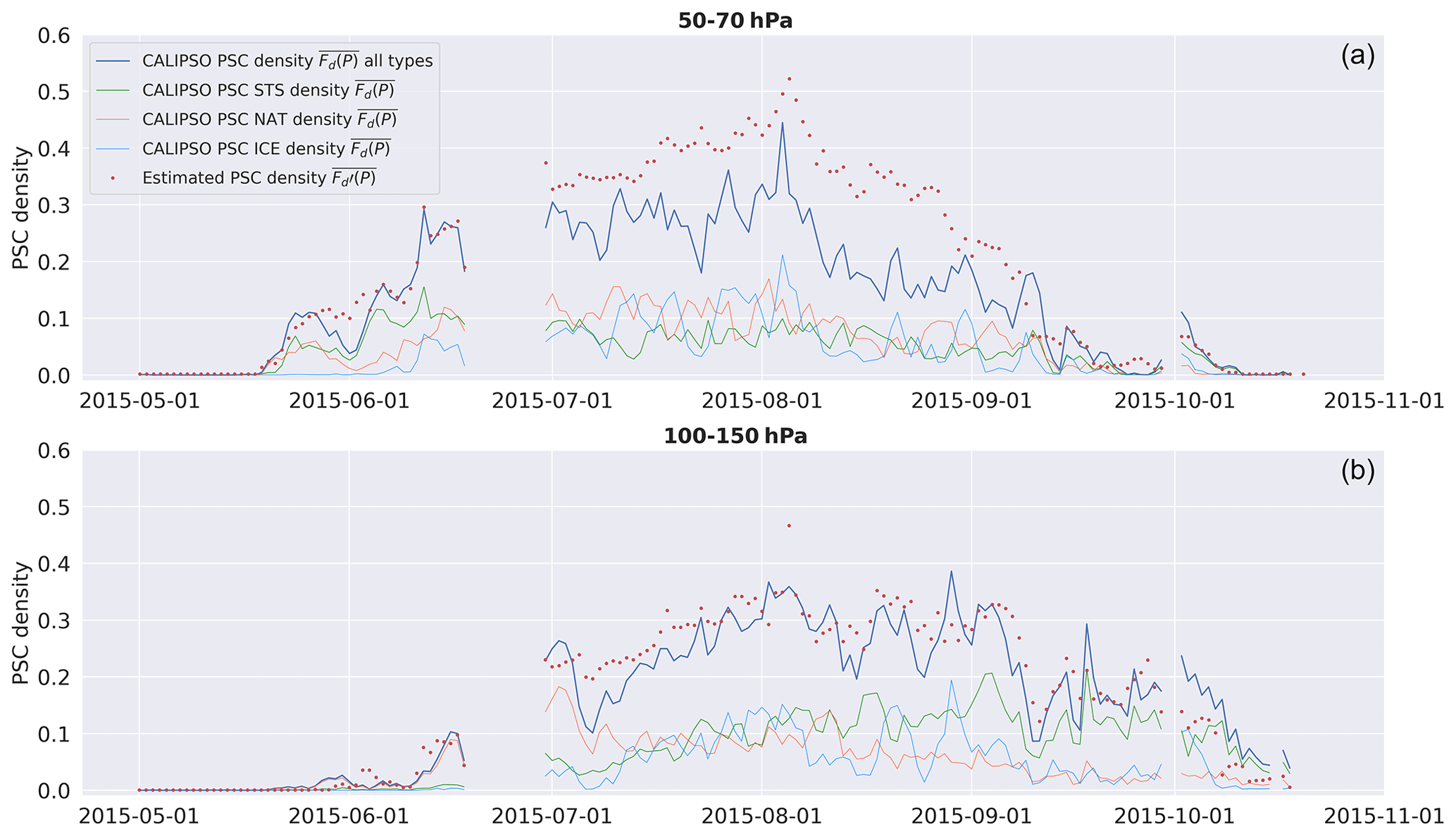
Figure E1 Time series of daily average PSC densities $\stackrel{\mathrm{‾}}{F_{\mathrm{d}}\left(P\right)}$ observed by CALIPSO (blue curve) and PSC densities estimated by our model $\stackrel{\mathrm{‾}}{F_{\mathrm{d}}^{\prime }\left(P\right)}$ (red dots) at 50–70 hPa (a) and at 100–150 hPa (b) for the year 2015. Colored lines represent the different PSC types. Green is for STS, orange for NAT, and blue for ICE.

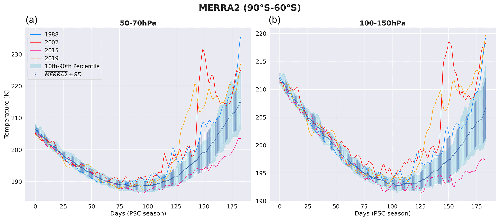
Figure E2 Daily MERRA-2 gridded stratospheric temperature average between 60–90° S and over each PSC season from 1980 to 2021 at 50–70 hPa (a) and at 100–150 hPa (b). The time series goes from 1 May (day 0) to 31 October (day 184). The mean of MERRA-2 (blue triangles) and its standard deviation (blue vertical lines) are shown.