Measurement report: Cloud and environmental properties associated with aggregated shallow marine cumulus and cumulus congestus

Mesoscale organization of marine convective clouds into linear or clustered states is prevalent across the tropical and subtropical oceans, and its investigation served as a guiding focus for a series of process study flights conducted as part of the Aerosol Cloud meTeorology Interactions oVer the western ATlantic Experiment (ACTIVATE) during summer 2020, 2021, and 2022. These select ACTIVATE flights involved a novel strategy for coordinating two aircraft, with respective remote sensing and in situ sampling payloads, to probe regions of organized shallow convection for several hours. The main purpose of this measurement report is to summarize the aircraft sampling approach, describe the characteristics and evolution of the cases, and provide an overview of the datasets that can serve as a starting point for more detailed modeling and analysis studies.

Six flights are described, involving a total of 80 dropsonde profiles that capture the environment surrounding clustered shallow convection. The flights include detailed observations of the vertical structure of cloud systems, comprising up to 20 in situ sampling levels. Four cases involved deepening convection rooted in the marine boundary layer that developed vertically to 2–5 km with varying precipitation amounts, while two cases captured more complex and developed cumulus congestus systems extending above 5 km. In addition to the thermodynamic and dynamic characterization afforded by dropsonde and in situ measurements, the datasets include cloud and aerosol microphysics, trace gas concentrations, aerosol and droplet composition, and cloud and aerosol remote sensing from high-spectral-resolution lidar and polarimetry.

1 Introduction

Cumulus convection is a pervasive component of the marine atmosphere above the global tropical and subtropical oceans (Warren et al., 1988; Johnson and Lin, 1997; Bony et al., 2004) where vertical transport and overturning circulations are tightly coupled to diabatic processes associated with radiative and latent heating (Riehl and Malkus, 1958; Johnson et al., 1999; Sobel and Bretherton, 2000). In addition to their role in the heat, moisture, and momentum budgets, convective clouds across all scales affect the production, loss, and vertical distribution of atmospheric trace gases (e.g., Dickerson et al., 1987; Fried et al., 2016; Li et al., 2018) and aerosol particles (e.g., Koch et al., 2003; Berg et al., 2015; Corr et al., 2016; Wonaschuetz et al., 2012; Reid et al., 2019; Leung and van den Heever, 2022). Tropical cloudiness has been associated with three major modes (Johnson et al., 1999; Haynes and Stephens, 2007): (i) a shallow cumulus mode often capped by a trade wind inversion; (ii) a middle mode associated with cumulus congestus and altocumulus, often associated with enhanced stability near the melting level (Posselt et al., 2008); and (iii) a deep mode (not considered here) associated with cumulonimbus and anvil cirrus, capped by the tropopause.

Oceanic regions that frequently accommodate deep convection are also subject to suppressed periods with shallow convection (Johnson and Lin, 1997; Malkus and Riehl, 1964). The vertical distribution and extent of clouds capable of supporting deep convection in unstable environments are also strongly dependent on the moisture profile (Redelsperger et al., 2002; Jensen and Del Genio, 2006; Takayabu et al., 2006) because of the inhibiting influences of entrainment and mixing on updraft buoyancy (Derbyshire et al., 2004). Indeed, pre-moistening of the mid-troposphere (Kuang and Bretherton, 2006; Waite and Khouider, 2010), upscaling of cloud-forming updrafts (e.g., through cold pools, Khairoutdinov and Randall, 2006), and moisture convergence (Hohenegger and Stevens, 2013) have been thought necessary to facilitate the growth from shallow to deep convection. For thermodynamic environments that lack pronounced stable layers (e.g., a demarcated cloud-capping trade wind inversion), separation of the shallow cumulus mode from growth into congestus may be more ambiguous and may be resigned to a subjective altitude threshold (e.g., 3–4 km). Similarly, a subset of clouds identified or classified as congestus may encompass nascent energetic growth of transient systems on its way to becoming deep convection (e.g., Luo et al., 2009), which may physically differ from terminal congestus where development has ceased (Leung and van den Heever, 2022).

In addition to understanding factors that control the vertical distribution of cumulus clouds, there has been a surge of recent interest in the spatial distribution of convection, particularly spurred by the propensity for deep and shallow convection to self-aggregate in cloud-resolving models under certain conditions. Simulations run close to a state of radiative–convective equilibrium over a homogeneous ocean surface can produce deep convection that progressively self-aggregates (Held et al., 1993; Tompkins, 2001; Tompkins and Craig, 1998; Bretherton et al., 2005; Muller and Held, 2012; Wing and Emanuel, 2014) and mimics the tendency of oceanic convection in the real tropical atmosphere to structurally organize across a wide range of horizontal length scales (Holloway et al., 2017; Mapes and Houze, 1993; Zuidema, 2003; Stein et al., 2017; Tobin et al., 2012; Semie and Bony, 2020; Masunaga, 2014; Nesbitt et al., 2006). Large-eddy simulations (LES) of shallow marine cumulus have been found to exhibit similar mesoscale self-aggregation of moisture and cloudiness, attributed purely to moisture advection and negative gross moist stability through model experiments that suppressed interactive radiation, surface fluxes, and precipitation (Bretherton and Blossey, 2017; Narenpitak et al., 2021; Janssens et al., 2023). In contrast, using LES experiments replicating conditions encountered during the Rain in Cumulus over the Ocean experiment (RICO; Rauber et al., 2007), Seifert and Heus (2013) found that cold pools from shallow cumulus precipitation were necessary to produce the organization of clouds into mesoscale arcs. Furthermore, shipboard observations during RICO confirmed the presence of frequent convective showers associated with shallow cumulus and their accompanying cold pools (Zuidema et al., 2012). Linkages have been made between precipitation-mediated shallow cloud organization and the influence of aerosols in modeling studies (Xue et al., 2008; Wang et al., 2010) and in observations (Wood et al., 2018; Mohrmann et al., 2019; Goren et al., 2019). A wide spectrum of shallow cloud organization types has been identified in nature, ranging from patterns found in stratocumulus (e.g., Wood and Hartmann, 2006), organization in mid-latitude cold air outbreaks (Agee, 1987; Atkinson and Zhang, 1996), fair-weather cumulus rolls (LeMone and Meitin, 1984), cloud patterns found in deeper boundary layers of the downstream trades (Schulz et al., 2021; Denby, 2020; Stevens et al., 2020; Janssens et al., 2021), and those associated with cold pools and congestus (Snodgrass et al., 2009; Zuidema et al., 2012; Rowe and Houze, 2015; Ruppert and Johnson, 2015). There is a clear need for continued observational efforts focused on cumulus aggregation to test and/or verify the findings from idealized numerical model simulations and to provide detailed observational support for the driving physical and dynamical processes across these various regimes.

Shallow cumulus clouds modulate albedo, and changes in their fractional coverage, vertical extent, and microphysical properties can exert a strong influence on regional and global climate (Bony et al., 2004; Vial et al., 2016; Rieck et al., 2012). In addition, the response of low-lying shallow cumulus, particularly in the trade wind regions, to climate warming constitutes a sizable uncertainty in climate model cloud feedback (Bony and Dufresne, 2005; Bretherton, 2015; Bretherton et al., 2013; Sherwood et al., 2014; Webb and Lock 2013). The amount of cloud coverage near cloud base (i.e., resulting from the contributions of very little cumulus) dominates the overall cloud fraction (Nuijens et al., 2014). Increases in convective mixing driven by increased mass flux in deeper, active cumulus projected to occur in future warming (Vial et al., 2016) have been postulated to result in desiccation of neighboring small clouds by entrainment drying (Brient and Bony, 2013; Sherwood et al., 2014; Brient et al., 2015), thus reducing the cloud base cloud fraction. However, recent analysis of trade wind cumulus observations has cast doubt on the strength of this feedback (Vogel et al., 2022), suggesting the importance of mesoscale organization of these clouds and of ubiquitous low-level mesoscale overturning circulations that drives the distribution of cloudiness (George et al., 2023). Variations in the type of mesoscale organization have been shown to result in changes in fractional coverage of shallow clouds and resultant cloud radiative effects (e.g., Bony et al., 2020), motivating the need for process-level understanding and effectual realization of their associated properties in climate models.

Microphysical properties of warm (ice-free) cumulus are controlled in part by the availability of aerosol particles to act as cloud condensation nuclei (CCN) and by dynamics (Kirschler et al., 2022). Clouds forming in higher-CCN environments result in smaller cloud droplets for fixed liquid water content (Twomey, 1977) that may delay and/or suppress the formation of precipitation (e.g., Rosenfeld and Lensky, 1998; Khain et al., 2005) and affect how cloudy parcels interact with their environment (e.g., Xue and Feingold, 2006). Retained cloud water and changes to the condensation rate may affect updraft buoyancy in competing ways (Igel and van den Heever, 2021; Grabowski and Morrison, 2021; Fan et al., 2018), affecting both shallow clouds that remain liquid only (e.g., Koren et al., 2014) and the potential for invigoration in the ice phase (e.g., Rosenfeld et al., 2008). In concert, these aerosol-mediated changes may influence the timeline of cloud growth, coverage, vigor, terminal vertical extent, and lifecycle precipitation (Koren et al., 2005, 2008; Tao et al., 2012; Igel and van den Heever, 2021; Barthlott et al., 2022; Fan et al., 2018; Rosenfeld et al., 2008; Storer and van den Heever, 2013; Khain et al., 2005; Marinescu et al., 2021).

Lateral and vertical mixing processes involving interactions between clouds and the surrounding environment are ubiquitous (Romps and Kuang, 2010) and exert control on the vertical distribution of cloud water (Rangno and Hobbs, 2005). Entrainment of subsaturated environmental air may influence the droplet population differently depending on the relative timescales of turbulent homogenization and microphysical response (Baker et al., 1980; Burnet and Brenguier, 2007; Jensen and Baker, 1989), which is a function of both the droplet sizes and the length scales of mixing (Kumar et al., 2018). The spatial and temporal heterogeneity of clouds, precipitation, and aerosols (and feedback therein) confounds efforts to understand aerosol–cloud interactions (Gryspeerdt et al., 2015; Varble et al., 2018), while aerosol effects on cloud microphysics may be modulated by the environment (Storer et al., 2010; Sokolowsky et al., 2022). Clouds also mediate the microphysical properties of subsequent clouds through their influence on pre-existing CCN properties (Hoppel et al., 1994; Feingold and Kreidenweis, 2000), the removal of CCN by rainout (Textor et al., 2006; Wang et al., 2020; Flossmann et al., 1985), and the lofting of precursor gases that nucleate new particles (Williamson et al., 2019). In summary, the myriad multi-path interactions amongst aerosols, clouds, radiation, and meteorology from the cloud system to the droplet scale may all contribute to the complexity of mesoscale aggregation of marine cumulus and motivate the need for targeted observations and further modeling.

In this paper, we present observational case studies associated with targeted aircraft measurements of aggregated shallow cumulus and terminal cumulus congestus that were conducted over the summertime subtropical western North Atlantic near the coastal United States and in Bermuda. Although this region is situated near the latitudinal extent of the tropics, sea surface temperatures (SST) are in a range close to typical of tropical basins (298–300 K), and low-level warm, moist advection driven by flow around the subtropical ridge produces air masses that are thermodynamically similar to conditions found in tropical maritime regions. These cases encompass a variety of mesoscale cloud conditions, exemplified by the nature of cloud organization and aggregation, vertical extent, macrophysical and microphysical properties, and environmental attributes, while occurring in relatively consistent larger-scale environments. The measurements include both in situ and remote sensing datasets from two coordinated aircraft platforms that specifically targeted regions of aggregated shallow convection. The main purpose of this measurement report is to summarize the aircraft sampling approach, describe the characteristics and evolution of the cases, and provide an overview of the datasets that can serve as a starting point for more detailed modeling and analysis of this set of case studies.

2 Methods and datasets

2.1 ACTIVATE

The Aerosol Cloud meTeorology Interactions oVer the western ATlantic Experiment (ACTIVATE) was conducted from the NASA Langley Research Center and from Bermuda during 2020–2022, comprising six airborne measurement campaigns split between winter and summer each year (Sorooshian et al., 2019). ACTIVATE employed a unique coordinated aircraft strategy for remote sensing and in situ sampling of clouds, aerosols, and trace gases that involved speed matching a turboprop King Air B200 or UC12 (King Air) at high altitude with a low-flying Dassault HU-25 Falcon jet (Falcon), allowing both aircraft to remain horizontally coordinated. Most flights used the coordinated aircraft in a survey pattern to build statistics (e.g., Kirschler et al., 2023), while a minority of flights were assigned to process studies during each season. During summer, process study flights were used specifically to probe organized regions of aggregated shallow cumulus and cumulus congestus, which were regularly occurring cloud patterns observed across the region.

Unlike statistical surveys where both aircraft prioritized following a single path, summer process study flights prescribed separate but coordinated patterns for each aircraft that were anchored to a target cloud system or convective feature (Fig. 1). At a nominal cruise altitude of 9 km, the King Air flew at least five transects across the target on different azimuths connected by shorter perimeter legs. Each transect nominally covered 80 km, with dropsondes released near the start and end of each transect to create a perimeter, as well as occasional placements near the center. Meanwhile, the Falcon performed a series of short, constant-altitude penetrations of the target cloud system and the near-field environment, repeated at multiple levels that also included a leg just above the highest cloud top and at least one leg below the lowest cloud base. Legs that penetrated cloud began close to cloud top, where there was typically a single emergent convective core, then progressively moved down in altitude, usually resulting in longer sampling legs as the cloudy region expanded to involve multiple cores, as illustrated schematically in Fig. 1a. The Falcon sampled the vertical structure of the surrounding environment, including one profile flown as a spiral located in a region completely free from any cloud, when possible.

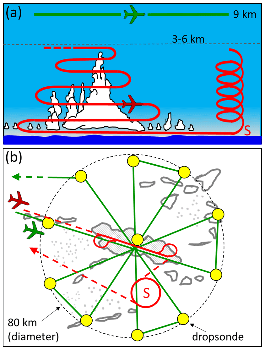
Figure 1 Schematic of the nominal two-aircraft flight strategy illustrating the position of the King Air (green) and the Falcon (red)/ (a) Cross section view of the altitude profile flown through the target cloud with adjacent clear spiral (S) and (b) plan view showing the “wheel and spoke” pattern.

A total of six process studies comprising individual research flights (RF) were conducted using this flight module design: (1) RF39 2020-09-29, (2) RF77 2021-06-02_L2, (3) RF80 2021-06-07_L2, (4) RF171 2022-06-10_L2, (5) RF173 2022-06-11_L2, and (6) RF176 2022-06-14 (note that following the archiving convention, L2 denotes the second flight of a given day). Here we will describe these respective flights as cases 1–6. Cases 1–3 were flown from the NASA Langley Research Center, and cases 4–6 were flown from Bermuda, where the project was based during June 2022. The flights originating from Bermuda benefitted from fewer airspace restrictions and shorter transit times to regions of interest, resulting in longer loiter times for sampling. Consequently, case 4 included a second cloud target that was fully sampled by the Falcon but only partially sampled by the King Air without additional dropsondes. Case 5 comprised two modules that included both aircraft, but the initial module was abbreviated by the Falcon because of rapid decay of the targeted cloud system. For instances where we wish to differentiate the two sections of these flights, they will be referred to as case 4A/B and 5A/B. Cases 1 and 6 occurred earlier in the day with module midpoints approximately 1 h prior to local solar noon (15:00–16:00 UTC) while cases 2–5 were later, occurring approximately 2–4 h after local solar noon (18:00–20:00 UTC) as a result of being the second flight of a two-flight day).

2.2 King Air

A multi-wavelength airborne high-spectral-resolution lidar (HSRL-2; Hair et al., 2008; Burton et al., 2018) provided vertically resolved aerosol and cloud properties below the King Air altitude. The HSRL-2 generates simultaneous measurements of the particle backscatter coefficient and depolarization ratio at 355, 532, and 1064 nm as well as the particle extinction coefficient at 355 and 532 nm, providing information about extensive and intensive aerosol properties. Aerosol type (marine, polluted marine, pure dust, dusty mix, smoke, fresh smoke, or urban) was derived using the depolarization ratio, spectral depolarization ratio, color ratio, and lidar ratio (Burton et al., 2012, 2014). Particle backscatter was used to diagnose the presence of liquid clouds and determine cloud top height at high vertical (∼ 1.25 m) and horizontal (∼ 60 m) resolutions.

The Research Scanning Polarimeter (RSP) is a passive, downward-facing polarimeter with nine spectral bands (410, 470, 550, 670, 865, 960, 1590, 1880, and 2260 nm) that scans along the direction of flight (nadir ± 55°), providing retrievals of aerosol, cloud, and surface properties (Cairns et al., 2003). During conditions with a narrow viewing-angle differential relative to the solar principal plane and absence of cirrus, the RSP was used to provide cloud top microphysical properties, including the drop size distribution for liquid clouds (Alexandrov et al., 2018).

The National Center for Atmospheric Research (NCAR) Airborne Vertical Atmospheric Profiling System was included on the King Air to acquire dropsonde observations, providing vertical profiles of temperature, humidity, pressure, and horizontal wind components. The dropsondes used here were the NCAR NRD41 “mini-sondes” (Vömel et al., 2021, 2023).

A nadir-facing camera (case 1 – Garmin VIRB Ultra 30 and cases 2-6 – AXIS F-1005-E) was mounted underneath the fuselage to provide continuous (1–2 s frame rate) images of the cloud scene. The AXIS camera was fitted with different lenses that changed the field of view amongst cases, resulting in a different footprint when viewed from 9 km. The camera images were also used to qualitatively diagnose the position of the aircraft during transects with respect to the target cloud system.

2.3 Falcon

Full details and specifications of the Falcon payload are described in Sorooshian et al. (2023), and here we provide a summary of the instruments. Water vapor was measured using an open path Diode Laser Hygrometer (Diskin et al., 2002), and temperature was obtained from measurements of total air temperature using a Rosemount 102 probe. Three-dimensional wind components were derived using a radome-mounted, inertially corrected five-hole gust probe (Thornhill et al., 2003; Barrick et al., 1996). Temperature, water vapor, and winds were acquired at 20 Hz. CO, CO₂, and CH₄ were measured using a near-IR cavity ring-down spectrometer (Picarro G2401-m; DiGangi et al., 2021), and O₃ was measured by a dual-beam ultraviolet absorption sensor (2B Technologies, Model 205), all at ∼ 2 s sampling interval.

Cloud droplet size distributions (DSD) were measured at 1 Hz using a Fast Cloud Droplet Probe (FCDP; SPEC Inc.) and a two-dimensional stereo (2D-S) probe (SPEC Inc.; Lawson et al., 2006) spanning 3–50 and 30–1500 µm drop diameters, respectively. The distributions from both instruments were merged at 1 Hz onto a uniform logarithmic grid (smoothed to 20 bins per decade), and a weighted average was taken in the overlap region (30–50 µm) with weights smoothly transitioning from FCDP to 2D-S. The linear-spaced size grid for the 2D-S based on pixel occultation results in low counting statistics for larger drops and is improved by re-binning. During cases 1 and 2, there were some periods where 2D-S data were not acquired, and precipitation DSD data from the Cloud Imaging Probe (CIP; Droplet Measurement Technologies) were substituted for the size range 500–1500 µm, which represented the only range where image analysis could be conducted for the CIP. Thus, during these periods no DSD data in the 50–500 µm range could be derived.

All clouds sampled by the Falcon in these process studies contained only liquid drops, as verified using particle imagery supplied by the 2D-S. The number concentration, N_d; liquid water mixing ratio, q_L; and precipitation rate were determined through integration of the DSD and terminal velocity data from Beard (1976), since in situ samples were verified as liquid drops. A notable caveat in relation to cloud phase exists for case 6, where liquid-only supercooled drops at ∼ −8 °C were observed near cloud top (∼ 5.6 km) at the time of initial Falcon sampling. The Falcon progressed downward in altitude to warmer temperatures while continuing to observe liquid-only conditions, but the cloud system was concurrently observed by the King Air to grow to ∼ 7 km (−15 °C). Hence, the presence of ice in this system cannot be discounted across its lifecycle despite no such indications from the Falcon observations. Cloud drop composition was directly measured through cloud water collection using an Axial Cyclone Cloud-water Collector (AC3; Crosbie et al., 2018), which usually resulted in one sample per cloud leg. These samples were analyzed offline for major ions, pH, and elemental composition.

Dry aerosol particle size distributions were measured using the combination of a Laser Aerosol Spectrometer (LAS; TSI Model 3340, 100–3000 nm diameter) and a Scanning Mobility Particle Sizer (SMPS; TSI Model 3085 DMA, TSI Model 3776 CPC, 3–100 nm diameter) stitched at 100 nm (Sorooshian et al., 2023). The LAS acquired size distributions at 1 s intervals, while the SMPS performed 45 s scans. Here we report size distributions as averages over time periods that include several SMPS scans. Condensation particle counters (CPC; TSI Model 3756 and 3772) provided ultrafine (> 3 nm) and fine (> 10 nm) total particle concentrations, with an additional fine CPC downstream of a thermal denuder at 350 °C providing non-volatile particle concentration (> 10 nm). A CCN counter (DMT Model 100; Roberts and Nenes, 2005) provided concentrations at 0.37 % supersaturation. Two integrating nephelometers provided dried and humidified (< 1 µm) particle scattering at 450, 550, and 700 nm wavelengths (TSI Model 3563). The CPCs, CCN counter, and nephelometers all provided data at 1 Hz. Non-refractory aerosol mass concentrations (< 1 µm) were measured at 30 s intervals using a high-resolution time-of-flight aerosol mass spectrometer (AMS; Aerodyne Research Inc.).

The FCDP was also used to characterize super-micrometer aerosol during sampling of clear air (q_L < 0.001 g kg⁻¹, no precipitation, and RH < 95%). This provided particle number and volume estimates (i.e., analogous to those described above for the LAS) at ambient conditions extending to larger sizes to aid in characterization of coarse aerosol.

The Falcon was also equipped with a forward-facing camera and a downward-facing Heitronics KT-15 infrared thermometer used to determine SST.

2.4 Auxiliary datasets

2.4.1 MERRA-2

Instantaneous (3 h) three-dimensional meteorological fields from the NASA Modern-Era Retrospective Analysis for Research and Applications Version 2 (MERRA-2; Gelaro et al., 2017) were used to provide supporting synoptic-scale data for the large-scale environment surrounding each case. Large-scale wind, temperature, humidity, and geopotential height data are available on interpolated pressure levels at 25 hPa intervals (in the lower troposphere) and at 0.625° × 0.5° grid spacing. Two-dimensional fields (surface pressure, sea level pressure, and surface geopotential) are provided on a coordinated grid and used to determine the lower boundary (e.g., for adjacent land masses) and to extrapolate the 1000 hPa geopotential height when below the surface. Precipitable water (PW) was estimated by trapezoidal integration of

$$\begin{array}{}\text{(1)}& \mathrm{PW}={\displaystyle \frac{\mathrm{1}}{g}}{\int }_{\mathrm{0}}^{p_{\mathrm{sfc}}}{q}_{\mathrm{v}}\mathrm{d}p,\end{array}$$

and the horizontal column moisture flux (MF) was similarly calculated using

$$\begin{array}{}\text{(2)}& MF={\displaystyle \frac{\mathrm{1}}{g}}{\int }_{\mathrm{0}}^{p_{\mathrm{sfc}}}{\mathit{U}}_{\mathbf{h}}{q}_{\mathrm{v}}\mathrm{d}p,\end{array}$$

where g is the gravitational acceleration, p (p_sfc) is (surface) pressure, q_v is the water vapor mixing ratio, and U_h is the horizontal wind vector. Contributions to the integral below 1000 hPa were included using the values of the fields at 1000 hPa.

Air mass trajectories were derived from the MERRA-2 horizontal wind fields averaged over a vertical slab between 950 and 800 hPa to reflect the dominant low-level horizontal motion. The air mass trajectory was solved numerically by integrating the slab wind forward and backward in time using a linear interpolation of the wind field to the trajectory location and time within the 3 h reanalysis outputs. This method of calculating trajectories intentionally ignores reanalysis vertical motion because the main purpose of the trajectories (in the backward direction) was specifically to assess surface source regions and history. Note that slab winds excluded the 975 and 1000 hPa levels to minimize sensitivity to reanalysis near-surface wind structure.

2.4.2 GOES-East advanced baseline imager

Visible (0.6 µm) satellite imagery from the Advanced Baseline Imager (ABI) on board the 16th Geostationary Operational Environmental Satellites (GOES-East) was accessed through the NASA Langley Satellite Cloud and Radiation Property Retrieval System (SatCORPS). The high-resolution (∼ 0.5–1 km pixel size) imagery was captured over the duration of each flight and relevant adjacent time periods at 20 min intervals.

2.4.3 Gridded sea surface temperature

Global daily Group for High Resolution Sea Surface Temperature (GHRSST) gridded data at a 0.01° spatial resolution were acquired for each flight (GHRSST Level 4 MUR dataset; last access October 18, 2022). The GHRSST dataset combines nighttime multi-platform satellite-retrieved products with in situ buoy SST measurements (Chin et al., 2017).

3 Synoptic environment

Backward trajectories (Fig. 2a) implied a tropical marine air mass origin (over a time period of 8 d) across all cases originating from the central or western tropical Atlantic and conforming to the expected climatological circulation around the subtropical anticyclone. Based on proximity to the North American continent, the air mass history of case 3 indicated the potential for contributions from continental pollution sources, and indeed trajectories extracted for higher altitudes (above 850 hPa; Supplement Fig. S1) indicated outflow from the eastern United States. Cases 1–3 were all located along the axis of the Gulf Stream (Fig. 2b), while the remaining cases were situated over more spatially uniform surface conditions near Bermuda. Data shown in Fig. 2b relate to case 6, but general SST spatial patterns were broadly consistent amongst the other cases (Fig. S2), with the caveat that case 1, which occurred in September, experienced regionally higher SST consistent with the seasonal cycle. The synoptic meteorological environment was broadly similar across cases, and an example of the large-scale pattern is shown for case 6 (Fig. 2c, d). The center of the subtropical anticyclone (as diagnosed by sea level pressure) was located to the east, and a quasi-stationary frontal boundary was located to the north, marking a region containing deep convection with enhanced PW and MF (Fig. 2d). Comparisons with other cases can be found in the Supplement (Fig. S3). During the majority of the summertime campaign, this frontal boundary was a persistent feature, with its position, strength, and characteristics modulated by transient mid-latitude systems, and was often anchored to surface features such as the Gulf Stream or the coastal region of the United States. Across cases, the relative position of these major synoptic features remained broadly consistent with respect to the location of the aircraft sampling, such that for cases 1–3 (located closer to the continent) the anticyclone was farther west with deep convection and frontal clouds generally found near the coast and onshore.

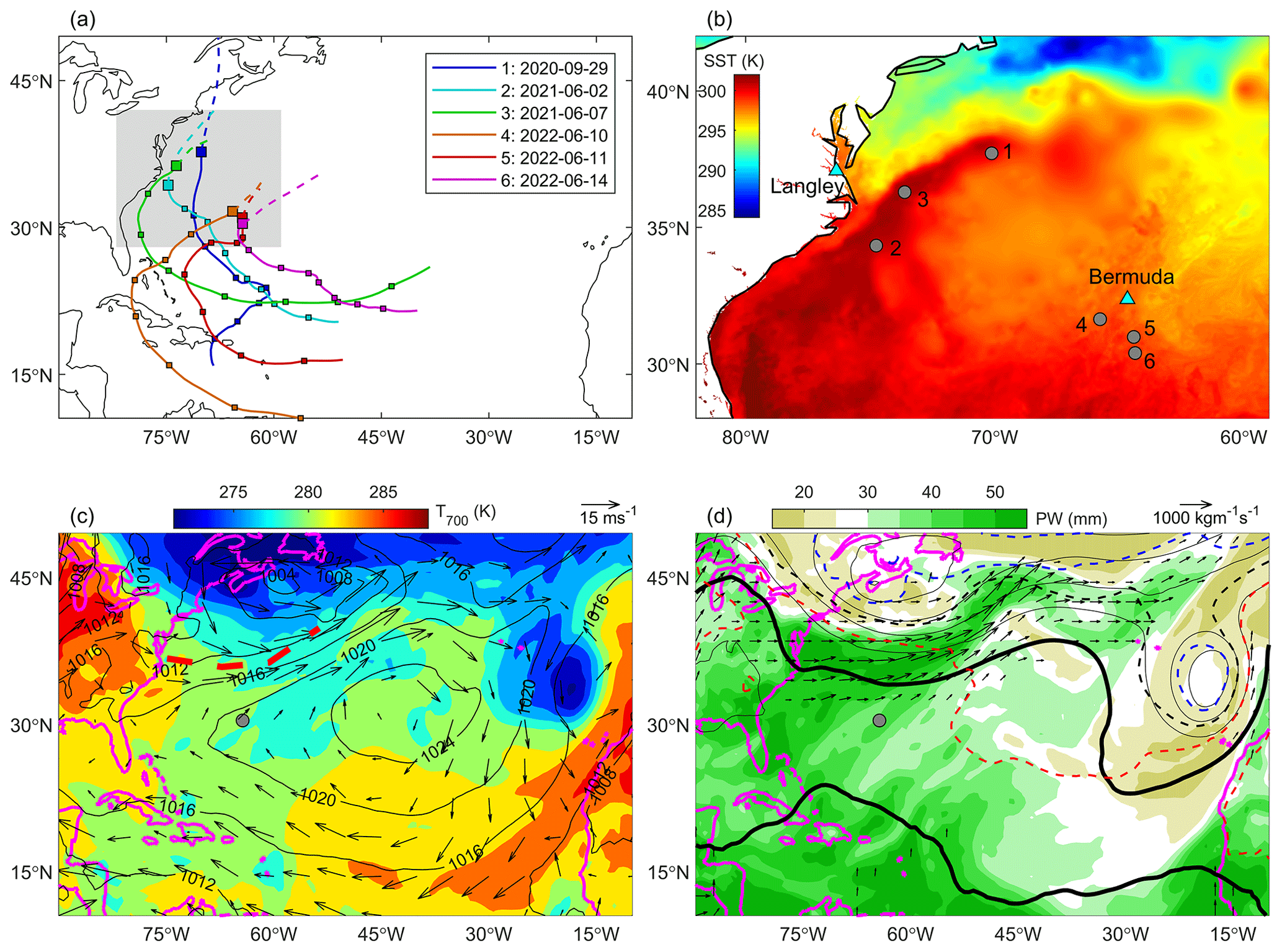
Figure 2 Large-scale meteorological environment. (a) 8 d back trajectory (solid) and 1 d forward trajectory (dashed) using MERRA-2 800–950 hPa layer averaged winds (see text) for cases 1–6. (b) Example SST shown for case 6 (14 June 2022) with all case locations shown for reference. The region in (b) corresponds to the grey-shaded region in (a). (c) Case 6 sea level pressure (contours), 850 hPa wind vectors, and 700 hPa temperature (colored). The location of the axis of the stationary front (see text) is shown by the thick red dash. (d) Case 6 PW (colored), MF (vectors), 500 hPa geopotential height (contours at 6 dm – decameter, 10 m – intervals; thick contour designates the 588 dm level), and 1000–500 hPa thickness – dashed contours at 6 dm intervals; black contour designates the 564 dm thickness line; red (blue) contours represent regions of higher (lower) thickness.

4 Mesoscale cloud organization and environment

4.1 Satellite tracking

Each process study flight module was fixed to a visually selected cloud feature that was used by both aircraft as a reference and defined as the center point of the sampling region. Satellite imagery taken near the midpoint time of each module indicated regions of enhanced cloudiness and visible cloud aggregation coordinated with the sampling region (Fig. 3), which was approximately bounded by the area spanned by the dropsondes (yellow dots). Apparent in cases 1 and 2 but also observed in cases 3 and 5 was the prevalence of very small cumulus fields elsewhere in the cloud scene and in the periphery of the enhanced cloud regions, together with the emergence of cloud-free zones often forming in the immediate surroundings. The position of the Falcon spiral profile (orange cross) was usually in one of these clearings 20–40 km from the cluster centroid. Contours of SST indicate the relative position of the module to the axis of the Gulf Stream in cases 1–3 and the comparatively homogeneous SST in cases 4–6. In cases 1 and 2, cloud sampling occurred above the ridge of maximum SST, while case 3 sampled the cloud system as it crossed the sharp gradient on its northwest edge (0.2 K km⁻¹).

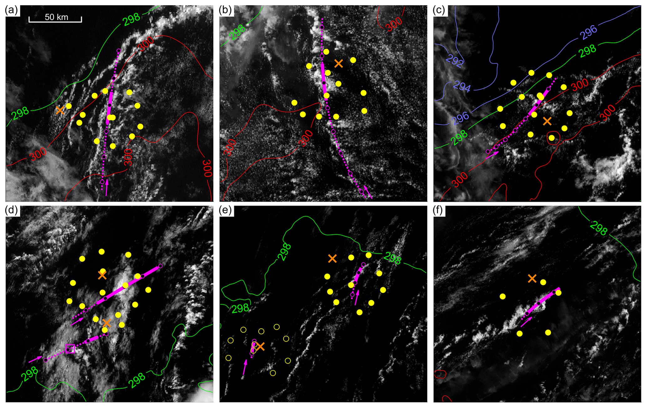
Figure 3 GOES-East ABI visible (0.6 µm) satellite imagery at the midpoint time of each process study. Panels (a–f) are cases 1–6, respectively, with a scale bar shown in panel (a). Overlaid on each panel – SST (K; contours), dropsonde locations (yellow dots), Falcon clear-spiral location (orange cross), and cloud cluster track (magenta). The cloud cluster track (see text) is separated into the time frame of the aircraft sampling (solid) and the remaining time window of the cluster lifetime (dotted). Hourly increments are shown as circles, and an adjacent arrow shows the direction of travel. Panels (d) and (e) are images from the midpoint of cases 4A and 5B, respectively. No dropsondes were associated with case 4B, but its cloud track is shown to the southwest of case 4A; the location of the tracked case 4B cluster at the time of the panel (d) image is marked with an open square. Dropsondes associated with case 5A are shown as open circles in panel (e), and the tracked cluster had already dissipated.

The cloud cluster anchoring each flight module was tracked using satellite imagery by calculating the maximum cross-correlation associated with sequential images for a region surrounding the cloud cluster (Nieman et al., 1997). Sequential images were analyzed forward and backward in time to estimate the lifecycle of the feature, and the displacements were fit using a least-squares regression to create a first-order (i.e., linear) prediction of the cloud motion zonal and meridional velocity components over the observed lifetime (Table 1). Satellite animations of the cloud scene evolution viewed in the derived (moving) reference frame of the cloud cluster are included in the “Video supplement” section.

Table 1 Cloud cluster sampling characteristics, lifecycle, and motion for cases 1–6.

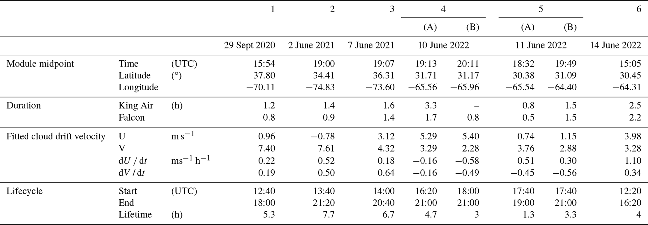
Table 2 Cloud and environmental properties of cases 1–6.

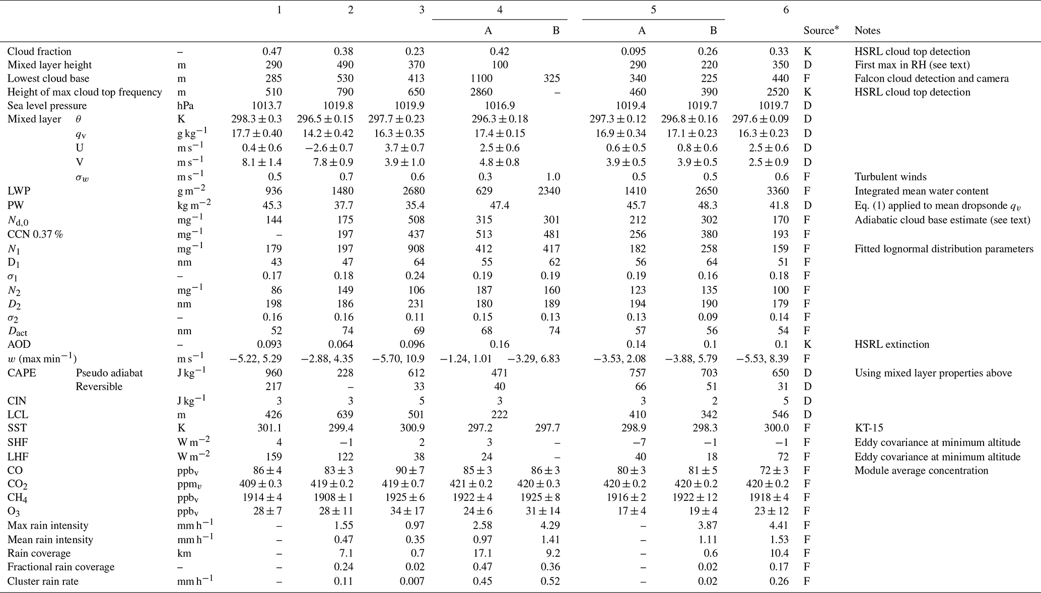
^* K – King Air observations; D – dropsonde; and F – Falcon observations

The longevity of each trackable feature varied from less than 2 h (the truncated case 5A) to more than 8 h. The lifecycles of cases 1 and 2 were less conclusive because case 2 was subsumed into deep convection, and case 1 likely shared the same fate but was first obscured by an over-running altocumulus deck approximately 2 h after the aircraft sampling concluded. The lifecycle of the other cases was more obvious because before and after there were either no clouds or limited/negligible aggregation. In case 4 (Fig. 3d) the image corresponds to the midpoint of the primary module (case 4A), which encompassed most of the mature lifecycle of this cluster. The secondary module located just to the south (case 4B) was part of the same mesoscale region, and the location of this cloud cluster at the time of the image is shown (marked “x”). Figure 3e shows the image at the midpoint of case 5B, which became the primary module due to the rapid decay of case 5A, whose clouds no longer existed at the time of the image.

4.2 Thermodynamic profiles

Mean dropsonde vertical profiles of potential temperature (θ; Fig. 4) show similar vertical structures amongst cases, in line with expectations for the summertime lower and middle troposphere in this region. Using case-specific parcel properties representative of the mixed layer, all layers contained moderate (marginal) convective available potential energy (CAPE) when implementing a pseudo-adiabatic (reversible) assumption (Table 2) and were associated with minimal convective inhibition (CIN), as is typical of tropical oceanic soundings (e.g., Betts, 1982; Xu and Emanuel, 1989). Although stable layers were present in some cases, notably case 1 (Fig. 4c), other cases (e.g., case 5) showed little change in stability with altitude. Based on stability alone, there were no indications from the environment precluding deeper convection from developing, and indeed, for all cases, satellite imagery indicated deep convective cells within 200–400 km.

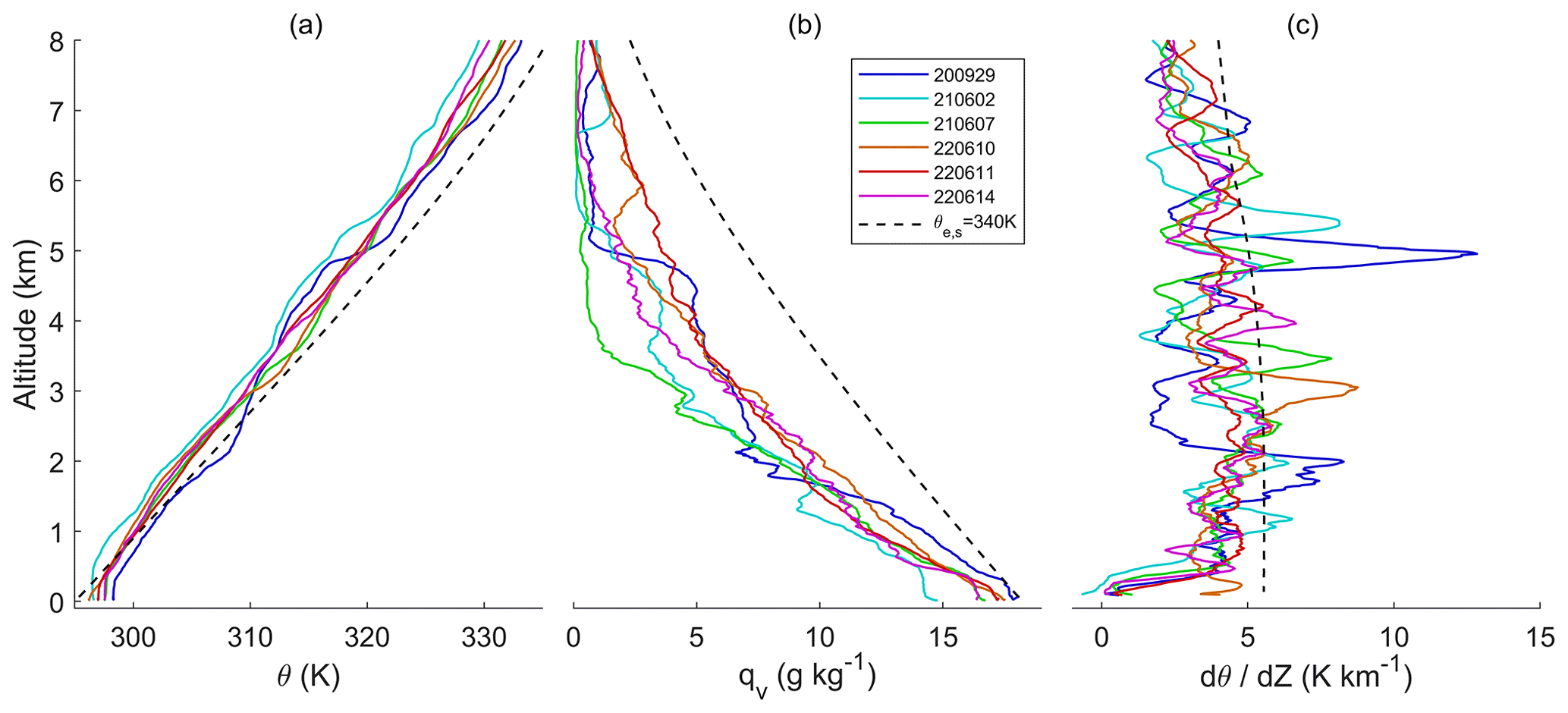
Figure 4 Case-mean dropsonde profiles of (a) potential temperature, (b) water vapor mixing ratio, and (c) static stability (defined as the vertical gradient of potential temperature and smoothed over a 100 m window). The profile of a reference wet adiabat corresponding to a saturation equivalent potential temperature (θ_e,s) at 340 K is also shown.

The mean water vapor mixing ratio (q_v) indicated more variability amongst cases, particularly in the 2–5 km altitude range, which coincided with the region of maximum saturation deficit (e.g., compared to the reference wet adiabat), and PW varied from 35 to 48 mm (Table 2). Overall, there was not a clear qualitative relationship between the details of the moisture profile and the size and extent of the cloud aggregation visualized by satellite (Fig. 3), a conclusion also drawn for organization of wintertime Atlantic trade wind cumulus (George et al., 2021). For example, case 5 exhibited the smallest cloud features with the least overall cloud coverage (Table 2), yet the environment of case 5B had the highest PW.

4.3 Winds

Wind profiles are shown in Fig. 5 as hodographs to visualize the effects of vertical shear of the horizontal wind and the winds relative to cluster motion. Relative winds can be visualized by shifting the origin to the cluster motion (square markers), and cloud layer shear can be represented by the vector from cloud base (downward-facing triangle) to top (upward-facing triangle). All cases indicate that cloud motion was close to the cloud base wind vector (within 1.3 m s⁻¹ relative vector magnitude), while the magnitude of the wind shear between cloud base and top varied from 1.6 m s⁻¹ (case 4) to 7.6 m s⁻¹ (case 2). In cases 1, 2, 5, and 6, the cluster motion was aligned (within 15°) with the major axis of cloud organization (indicated as a dashed line in Fig. 5), but only in case 6 was there an absence of any directional shear such that the cluster motion, the shear vector, and the major axis were all aligned. Cases 1 and 5 exhibited several near-parallel linear cloud features (“cloud streets”) and shared a similar near-perpendicular shear vector across the depth of the cloud, and it is notable that pronounced linear organization occurred in case 5 despite both weak mean flow and shear. Shear was almost nonexistent in case 4 along with only marginal directional organization of cloud features within the module, although there was evidence of cloud banding at a larger scale (∼ 1000 km) along a north–south axis east of the module. Case 3 was the only example where the cloud formed a pronounced linear (∼ 40 km) feature that was oriented approximately perpendicular to the cluster motion and the shear vector, although satellite imagery also indicated that this was part of a larger (∼ 200 km) organizational pattern of interconnected rings extending along the Gulf Stream axis to the northeast.

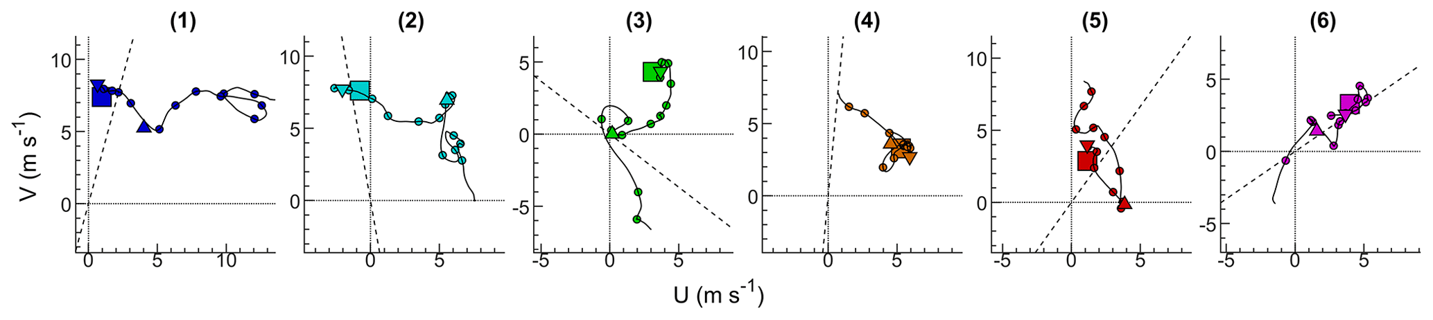
Figure 5 Case-mean dropsonde wind profiles displayed as hodographs for cases 1–6. The wind profile is smoothed with a 25 hPa running mean and markers (circle) indicate increments of 50 hPa. Also included are winds at cloud base (downward-facing triangle) and cloud top (upward-facing triangle; estimated based on the top of the Falcon module), the mean cluster motion from satellite imagery (square), and the primary axis of cloud organization estimated from satellite imagery (dashed line). In each panel the scale is preserved, with the position of the origin shifted to center the data. Case 5A dropsondes are omitted from (5) for readability but show a similar structure to case 5B (shown).

5 Cloud properties

5.1 Cloud height distributions

Frequency distributions of the heights of cloud tops detected by HSRL-2 during the King Air module (Fig. 6) indicated that in four of the cases (cases 1–3 and 5), a pronounced peak in frequency occurred below 1 km with a near-monotonic decrease with altitude in the 1–2 km thereafter. Across these four cases, the modal altitudes were 100–200 m above the altitude of the lowest cloud base determined from the low-flying Falcon (Table 2) and reflected the relatively high occurrence of very small cumulus anchored atop the marine sub-cloud mixed layer that prevails in peripheral regions surrounding cloud clusters despite the apparent emergence of clearings on satellite imagery. The small, optically thin clouds captured by the lidar may be more pervasive than indicated by visible satellite imagery (Mieslinger et al., 2022). Mixed layer depths (Table 2) were determined from the altitude of the first maximum in relative humidity of the mean dropsonde profile, which also corresponded to the inflection altitude where mean θ (q_v) substantially increased (decreased; Fig. 4), and were found to be within 50 m of the lowest cloud base. Across these four cases, the lowest lifting condensation level (LCL) determined from the mean dropsonde data was found 70–140 m above the lowest cloud base and was attributable to variability in temperature and humidity, while increases in mixed layer depth and the cloud base correlate with increases in the cloud top modal altitude at a degree slightly higher than proportional (1.2), indicating a minor thickening of the small cloud mode with increasing sub-cloud depth.

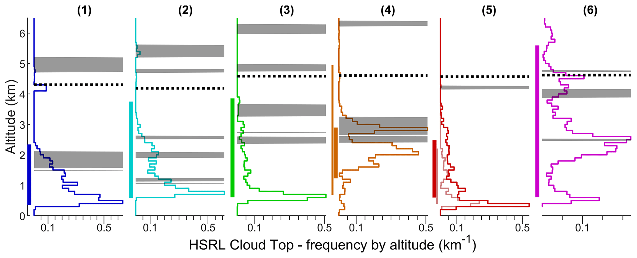
Figure 6 Frequency distributions of HSRL-detected cloud tops for cases 1–6. Frequency data are normalized by the total available records within the module, such that an integration of the distribution results in the HSRL cloud fraction (Table 2). Also shown are regions where dθ / dz exceeds 6 K km⁻¹ as an indicator of stable layers (grey shading) and the 0 °C level (dashed). The vertical bar adjacent to each case indicates the span of altitudes sampled in situ by the Falcon and in panels (4) and (5) shows the altitude span for the secondary Falcon modules (thin bar; cases 4B and 5A, respectively).

In stark contrast, the dominant cloud top modes for cases 4 and 6 were at 2.9 and 2.5 km, respectively. The vertical distribution of clouds was fundamentally different in these cases, and pronounced local maxima in the frequency of cloud tops were observed within multiple altitude ranges, while cloud tops observed below 1 km were less frequent, most notably for case 4. Undoubtedly, some low-lying clouds may be obscured by laterally spreading cloud aloft, and these cases also generally sustained less small cumulus in the surrounding environment, as indicated in Fig. 3 and as confirmed by in-flight camera imagery. The observations indicate that regions of enhanced stability do not exert an obvious controlling influence on the distribution of cloud tops, except in case 4. Regions of the column with static stability exceeding 6 K km⁻¹ (shaded in Fig. 6) would tend to inhibit further cloud growth, creating the expectation for more cloud tops to be found within those regions. However, local maxima in cloud top frequency are almost equally located above, below, and within stable layers, while some stable layers result in no apparent influence on the vertical distribution at all.

The 0 °C altitude (marked in Fig. 6) has been attributed to a stability enhancement (e.g., Posselt et al., 2008), but in these six cases there was not a conclusive association between stability and the region close to the 0 °C level; however, cases 1 and 6 (and marginally case 4) indicated some partiality for cloud tops at that level. It is worth noting that the clouds detected above 4 km in case 1 were mostly associated with altocumulus that was not coupled to the convection below, except in one region (confirmed via camera imagery) that was associated with a short-lived deeper convective cell offset from the Falcon's sampling region. In contrast with the apparent influence seen in case 6, case 2 did not show any relationship between clouds, stability, and the 0 °C level, while no clouds were observed to reach that level in cases 3 and 5. The cloud tops observed above 4, 3, and 6 km in cases 2, 5, and 6 were determined to be associated with emergent growth of convective turrets that occurred after the start of the Falcon module, and so those altitudes were not sampled in situ. Less cloud was observed at all altitudes during case 5A compared to 5B, in agreement with the initially small size of this cluster at the onset of the module and the subsequent decay. Cloud height distributions can also be visualized using the HSRL-2 backscatter curtain plots, which are included in the Supplement (Fig. S4).

5.2 Vertical velocity

Figure 7a shows statistics of the vertical distributions of vertical velocity, w, measured in situ for each case. Each level leg was truncated to remove maneuvers and was high-pass filtered (50 s FFT filter) to remove low-frequency biases/drift and any residual airframe dynamical effects. A q_L-weighted mean was calculated for w, which represents a characteristic velocity for the convective transport of condensed water (here w_L is used to differentiate this quantity specifically). The spread of w, indicated by the 10 %–90 % range, quantifies the relative magnitude of cloudy updrafts and downdrafts (filtered for clouds; q_L > 0.02 g kg⁻¹).

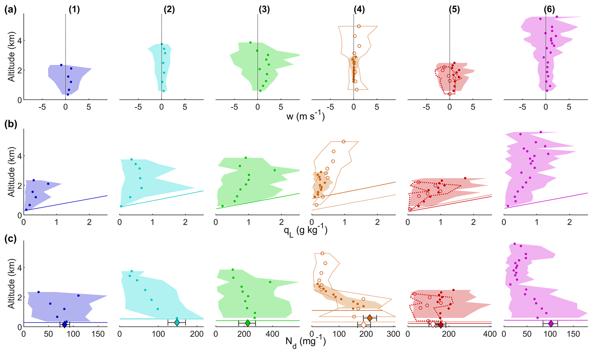
Figure 7 Statistics of in-cloud properties measured in situ for cases 1–6. (a) Vertical velocity, w; (b) liquid water mixing ratio, q_L; and (c) drop number concentration, N_d. The shaded region corresponds to the 10 %–90 % range, and dots are the transect mean values where data are filtered for clouds using q_L > 0.02 g kg⁻¹. In the case of (a), the transect means are calculated as a q_L-weighted mean referred to as w_L in the text. Also shown in (b) is an adiabatic parcel initialized from saturation at the lowest cloud base, shown as a horizontal line in (c). Also shown in (c) is a reference aerosol concentration based on the particle number concentration exceeding 100 nm in diameter measured during sub-cloud sampling (marker – mean; bar – 10 %–90 % range). In (4) and (5), data for the secondary modules are included (case 4B and 5A, respectively) and are shown by dashed lines and open markers.

Across the cases, maximum updrafts varied between 1.1 m s⁻¹ (case 4A) and 9.9 m s⁻¹ (case 3), while maximum downdraft magnitudes varied between 1.1 m s⁻¹ and 6 m s⁻¹ (the same cases, respectively). Updraft and downdraft extrema were all located within 850 m of the highest in-cloud transects, but because cloud top was dynamically evolving, it was challenging to classify this level as a fraction of cloud depth. Transects that encountered stronger updrafts also contained stronger downdrafts, resulting in a correlation coefficient of −0.77 between updraft and downdraft velocity. The mean updraft velocity exceeded the mean downdraft by 17 % in magnitude.

Positive w_L occurred in 82% of cloud transects and corresponds to a conventional expectation of strong upward flux of cloud water in the convective core, with subsiding motion in diluted (i.e., lower q_L) peripheral regions and in the immediate cloud-free environment. Negative w_L occurred predominantly near cloud top in a subset of cases and is believed to be an entirely transient characteristic of individual convective turrets because the source of cloud water is condensation in updrafts. Transient negative w_L may occur when cloud parcels descend after having overshot neutral buoyancy or because of negative buoyancy generated through homogenization of entrained air. While a descending cloud top interface does not necessarily require negative w_L, transient negative w_L is associated with a cyclical collapse of cloud top, and this was observed visually during flight, most prominently in case 3. Here, the upper extent of the cloud rapidly evaporated and descended approximately 1 km in 5 min, as diagnosed by forward camera imagery, thus implying a cloud top recession velocity of ∼ −3.3 ms⁻¹ compared to the observed w_L of −1.6 ms⁻¹ measured during the uppermost transect. Case 5A contained the highest occurrence of negative w_L, and within 15–20 min there was no visual evidence of the cloud system, which was confirmed by visible satellite imagery. These cases are too limited in number to provide a statistical description of the behavior of an ensemble of cloudy thermals within a typical system, but the occurrence of transient negative w_L here may be amplified as a consequence of the flight strategy. Emergent convective turrets that were used to anchor the sampling were identified with a lead time of several minutes, so there was a greater (than typical) chance that a selected turret would subsequently be in decline by the time sampling of the cloud top region was underway. Evidence of thermal bubbles exists in the vertical structure of w_L, particularly for case 3 and the upper half of case 6. Regions where w_L was close to zero also tended to occur in parallel with local reductions in the strength of updrafts and downdrafts at that level and are attributed to wake regions detrained from active thermals. While residual turbulence remained in these regions, parcels may be closer to neutral buoyancy, representing the more aged regions between rising bubbles or regions where cloud had spread laterally. Beyond the scale of single transects and individual thermals, case 4A (which was sampled immediately after deeper convection had ceased) exemplifies this at the cloud system scale, with minimal w_L and weaker updrafts and downdrafts, in agreement with the observed lack of surface-coupled convection and a more stratiform appearance.

5.3 Liquid water content

Vertical gradients of q_L capture the rate of condensation mediated by the effects of dilution and evaporation from entrainment alongside losses due to precipitation. An adiabatic q_L from a parcel released at the observed lowest cloud base for each case (included in Fig. 7b) represents an estimate of the q_L resulting from condensation alone, generally providing an upper bound. Near cloud base, q_L increased with altitude, with some cloudy parcels initially approximating the adiabatic parcel. With altitude, the envelope of q_L (as quantified by the upper 90 % bound) generally increased at a slower rate (cases 1, 4B, and 5), exhibited little trend (cases 3 and 6), or reverted to a decrease (case 2). The highest q_L was observed in case 3 (2.7 g kg⁻¹) despite the fact that the environmental humidity was lowest (Fig. 4b). For some upper cloud regions, q_L tended to fluctuate between adjacent sampling levels, and this was most notable in case 6, perhaps accentuated by the cloud system depth and the high number of cloud transects. This pattern is indicative of snapshots through an ensemble of transient convective elements (e.g., Morrison et al., 2020), where a chain of several rising thermals occurs sequentially, with each evolving in time such that the aircraft transects reflect different stages of their lifecycle, proximities to their cores, and energetic characteristics. In these dynamic environments, the aircraft measurements cannot singularly isolate vertical variability but rather incorporate the temporal evolution of individual thermals and the cloud system at large. Despite uncertainty in segregating time evolution and spatial scales of variability, the aircraft snapshot confirms an intermittent structure for emergent cores rather than a stationary plume, while at lower altitudes the data are more reflective of the larger ensemble of contributing thermals at each level.

5.4 Cloud droplet number concentration

The overall trend was for droplet number concentration (N_d) to decrease with increasing altitude, except in case 5 where a minor increase was observed (Fig. 7c). In cases 1 and 3, the trend in N_d was punctuated by locally anomalous high concentrations at 2.1 and 3.0 km, respectively, corresponding to local enhancements in the profile of q_L that were attributable to fresh, energetic convective bubbles. In the absence of these singular outliers, cases 1–3 (and case 6 below 2.5 km) indicated near-monotonic decreases at a rate of between 27% km⁻¹ and 52% km⁻¹. Comparison of the mature/decaying (4A) and active/developing (4B) systems of case 4 showed very close agreement in average N_d across commonly sampled altitudes, indicating robustness in the structure of the profile and suggesting that temporal evolution of horizontal mean N_d may not be substantial over the system lifecycle for a congestus complex such as in case 4. Cases 4B and 6 exhibited similar vertical patterns with decreasing N_d found below 3 km and with subsequent increases to a secondary maximum aloft at 4.3 and 4.6 km, respectively.

The source of N_d at cloud base is the activation of aerosol particles that serve as cloud condensation nuclei (CCN). The number concentration of particles with diameters exceeding 100 nm (N_a,100) was used as a proxy for the availability of CCN, qualitatively capturing the variability in N_d amongst the cases. The N_d for case 5A (decaying) was 45 % lower than case 5B (active) but coincided with a 22 % decrease in the below-cloud N_a,100. The fact that the change in N_d was proportionally greater than the change in aerosol may be explained partly by weaker cloud-forming convective updrafts in case 5A, even though the sub-cloud turbulence was found to be similar (Table 2). The contrasting N_d behavior seen in case 5 compared to the consistent N_d characteristics in case 4 highlight the different roles of aerosol interactions across lifecycle for different cloud system types. Crucially, a greater desiccation by entrainment because of its smaller size and lack of fresh convection was likely controlling the statistics of N_d observed in case 5A. In an attempt to separate initial activation (a topic that will be discussed further in Sect. 7) from subsequent in-cloud controls on N_d variability, a reference concentration (N_d0) was calculated from air parcels near cloud base that indicated recent droplet activation (Conant et al., 2004). Here, N_d0 (Table 2) was computed as the mean of data points collected in the lowest two cloud transects, limited to updrafts free from precipitation, and with q_L within 80 % of the reference adiabatic parcel representing a best estimate of the initial cloudy state. The q_L criterion was relaxed to the maximum observed adiabatic ratio when no data above 80 % occurred. The lowest N_d0 was found for case 1 (144 mg⁻¹) and the highest for case 3 (508 mg⁻¹).

N_d data were normalized by N_d0 and then compared to the ratio of q_L and the adiabatic water content (Fig. 8), representing a comparison between the observations and an idealized adiabatic parcel. Phrased another way, these normalizations are the fraction of drop number and mass concentration retained, compared to an undiluted parcel ascent. Mean properties from each transect (Fig. 8a) indicate that reductions in q_L result in proportionally smaller changes in N_d, such that 96 % of the transects lie above the 1:1 line. For clarification, a 1:1 relationship would indicate that number and mass are equally affected by dilution and evaporative losses, suggesting either extreme inhomogeneous mixing or partial volumes of cloudy and clear air at the scale of the measurement (∼ 100 m). There is no strong divergence or separation in the behavior between cases, indicating some degree of universality: the combined data exhibit a positive correlation coefficient (R= 0.73), and a total least-squares linear regression indicates a slope of 1.89. The joint frequency of 1 s cloudy data (rather than transect means) across all cases (Fig. 8b) confirms the same enhancement of N_d over a 1:1 relationship and, for the lower range of q_L that comprises the majority of the data, suggests that a linear model is appropriate, noting that logarithmically spaced bins were used to better reflect the distribution of data points. At higher q_L, the use of 1 s data shows the distribution asymptotes towards N_d0, in line with expectations for data to terminate around (1, 1) by design. Although data points that are close to adiabatic represent a small set of the total observations, separation by vertical velocity (Fig. 8c) indicates that this region of the joint histogram is more influenced by updrafts.

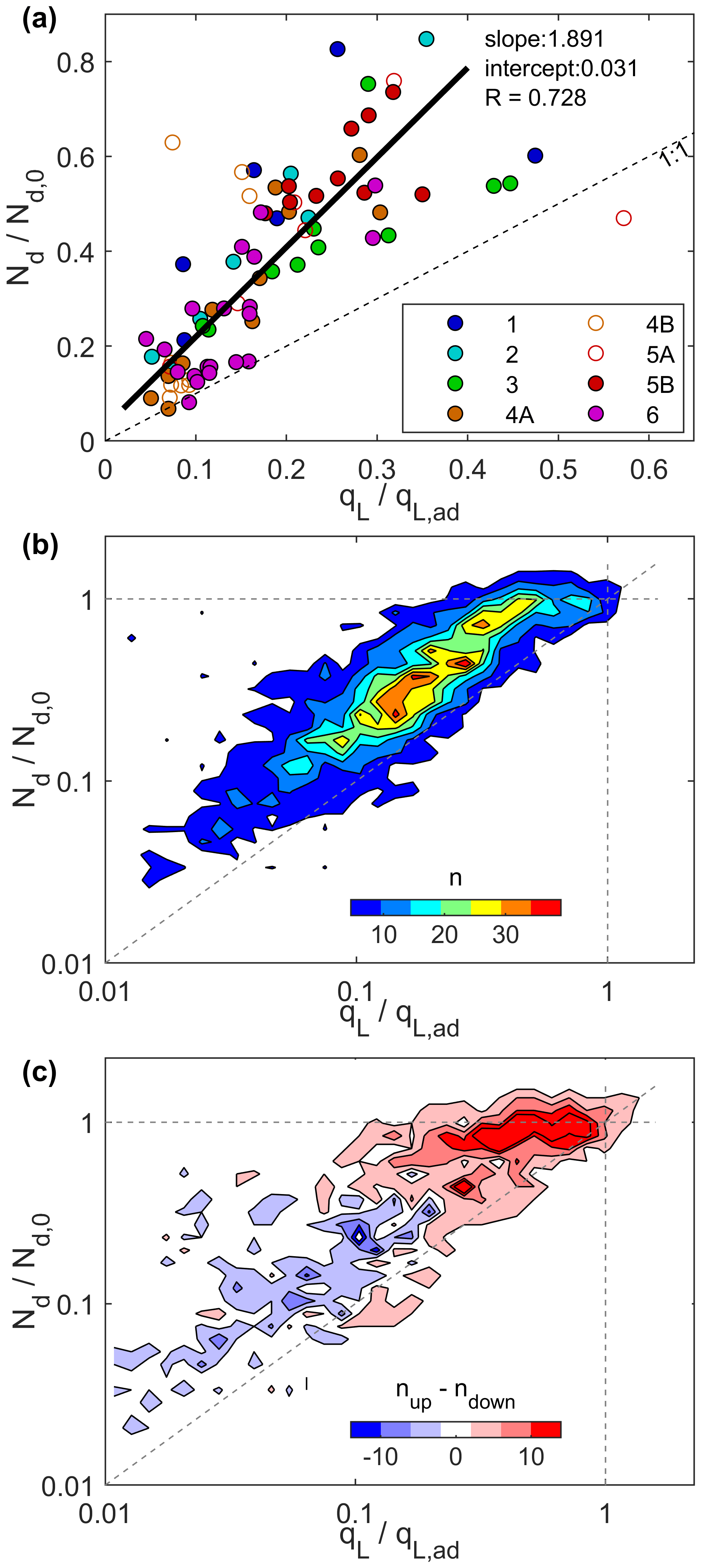
Figure 8 Variation in N_d and q_L with respect to a reference parcel with properties N_d,0 and q_L,ad. (a) Transect in-cloud mean for cases 1–6 (open circles for secondary modules). A linear model is fit to the data using total least squares with equal uncertainty in q_L and N_d. (b) Joint frequency distribution (counts; n) of all cloudy data for all cases with logarithmically spaced bins. (c) Same as (b) but showing the difference in the joint frequency distribution between updrafts and downdrafts.

All else held constant, droplet collisions would reduce N_d without changing q_L, while loss of q_L by accretion of falling precipitation would have a near-equivalent impact on N_d notwithstanding a strong size dependence of collection efficiency. Therefore, the results shown in Fig. 8 indicate that collisions cannot be dominant in shaping the budget and vertical distribution of N_d, particularly for updrafts.

5.5 Drop size distributions

Anomaly drop size distributions (DSD) were derived from the mean DSD from each cloud leg, normalized by leg mean N_d, and then compared as a ratio to the normalized mean of all cloud legs (Fig. 9). The resulting anomaly DSD vertical profile represents relative enhancements or reductions in the DSD shape compared to the reference DSD shape, without conflating changes in N_d. The advantage of this approach is that anomalies can be assessed independently of the drastic change in number concentration that occurs over the entire DSD (i.e., both cloud water and rainwater modes). At each level, the DSD exhibits the combined influence of net condensation, entrainment and subsequent mixing of environmental air, secondary droplet activation, collisions amongst cloud droplets, and the removal of drops by falling precipitation. A monodisperse reference drop diameter was calculated using N_d0 and q_L,ad to represent idealized behavior of a reference adiabatic parcel and is overlaid on Fig. 9.

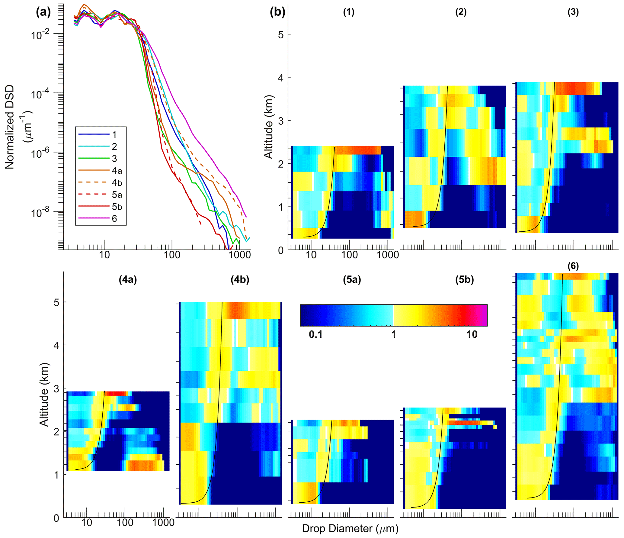
Figure 9 Vertical profile of the anomaly-normalized drop size distributions (DSD). (a) Reference normalized DSD calculated from the mean across all levels sampled. (b) For cases 1–6 at each level, the transect mean in-cloud DSD is normalized to unit integral, and then the anomaly is calculated as a ratio to the reference DSD. Warm (cold) colors therefore represent a higher (lower) than average contribution to the DSD shape, and use of the anomaly permits comparison across the size spectrum despite the large change in concentration. Also shown for each case is the monodisperse drop diameter of an adiabatic parcel (black line) initialized at the lowest cloud base with a drop number concentration, N₀ (see text).

We observe three major modes that vary in their degree of significance amongst cases: (i) a condensation/evaporation mode that resembles a “J” shape and closely but not identically aligns with the reference monodisperse diameter and could represent upward or downward motion, (ii) a precipitation growth mode that when coupled with the upper section of the “J” forms an inverted “V” and reflects rain drop growth caused by accretion, and (iii) a secondary activation mode that occurs to the left of the “J” and may occur at multiple altitudes.

Positive anomalies associated with mode (i) often track close to the monodisperse adiabatic diameter, even with the sub-adiabatic profile of q_L (Fig. 7b), and more importantly despite the proportional enhancement of N_d (Fig. 8). Extreme inhomogeneous mixing of entrained environmental air would tend to affect N_d and q_L equally by completely evaporating a subset of drops while the remaining drops retain their size (Jensen and Baker, 1989). Conversely, homogeneous mixing reduces the size of all drops and, in isolation, could offer a partial explanation for the behavior shown in Fig. 8, where drops lose cloud water or do not grow as fast (reduced $q_{\mathrm{L}}/q_{\mathrm{L},\mathrm{ad}})$, but with a lesser impact on N_d (less reduced $N_{\mathrm{d}}/N_{\mathrm{d}\mathrm{0}})$. However, the near-adiabatic growth of mode (i) shown in Fig. 9 would contradict the assertion, instead indicating that a subset of droplets was shielded from the influence of entrainment. The majority of 1 s observations (sampling interval) show that q_L remains distinctly sub-adiabatic, even at the 90 % level (Fig. 7b), suggesting that any regions of undiluted growth manifest predominantly at scales < 100 m (sampling interval times flight speed).

Mode (i) is often accompanied by additional smaller drops (i.e., explaining the enhanced N_d behavior of Fig. 8) that sometimes are concentrated at specific sizes (i.e., as mode iii). In addition, the reference normalized DSD in Fig. 9 shows pronounced multimodal characteristics that would not be as distinct if it were only representing the averaged growth with altitude of a single broadened mode. While some contributions to mode (iii) may result from mixing that is effectively homogeneous at the smallest scales but inhomogeneous at larger scales (but still < 100 m), the magnitudes of the enhancements in mode (iii) are suggestive of episodic, distinct secondary droplet activation (i.e., events that take place above the lowest cloud base).

The broadening of the DSD with altitude, implied by Fig. 9 through the emergence of modes (i) and (iii), was investigated quantitatively using the relative dispersion, ϵ, which relates the standard deviation of the drop sizes comprising the DSD to the mean size (Tas et al., 2015). As a number-based measure of DSD broadening, the magnitude of ϵ is insensitive to the tail of DSD and therefore not directly impacted by processes relating to precipitation (i.e., the role of mode ii). Amongst cases, ϵ exhibited similar values (Fig. 10), showing a consistent increase with altitude (0.075 km⁻¹). Across the data, the average ϵ was 0.47±0.12, which is higher than was reported for cumulus over land (Tas et al., 2015), potentially because their cases were shallower and more polluted. Furthermore, the updraft dynamics of daytime cloud-forming thermals over land may result in fundamentally different entrainment–microphysics interactions compared to these marine cases. In summary, significant DSD broadening is attributed to entrainment processes: specifically the combination of inhomogeneous or incomplete mixing of rising parcels together with activation of additional droplets within the time that mixing is taking place.

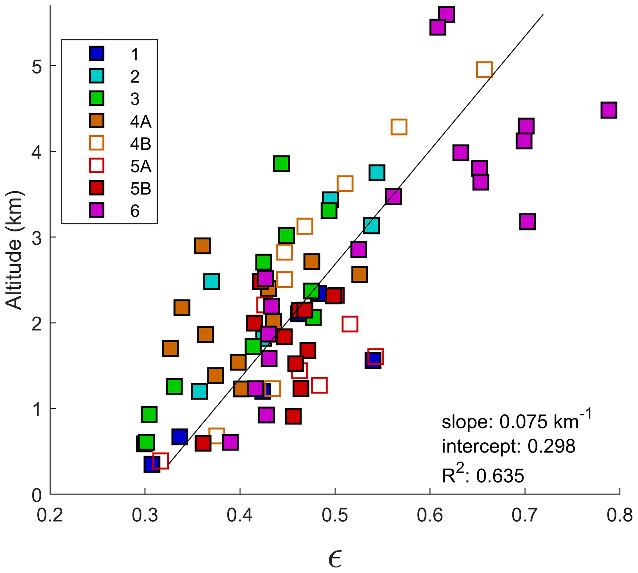
Figure 10 Profiles of DSD relative dispersion, ϵ, for cases 1–6. Values of ϵ are calculated locally at the measurement interval (1 s; ∼ 100 m) and then averaged (weighted by N_d) across a transect.

In all cases there was evidence of precipitation initiation/formation near cloud top, attributed to an active collision/coalescence process causing growth of the anomaly DSD well beyond the adiabatic diameter (Fig. 9). However, the emergence of subsequent precipitation growth (mode ii) was most prominent in cases 2, 4B, and 6, although each case exhibited a marked decrease in the significance of this mode at lower levels. Part of the decrease in the rain mode was attributed to the higher fractional contribution of non-precipitating clouds that did not extend beyond lower altitudes (Fig. 6), but it is notable that some cases (3 and 4A) exhibited distinct breaks in the precipitation growth mode and may represent the temporal and spatial intermittency of convective transport.

A hypothesis for the rapid decrease in the precipitation mode at lower levels (seen most prominently in case 3) is that the time needed to produce precipitation and enact sufficient growth is in direct competition with the buoyancy “clock” of cloudy volumes, which are progressively succumbing to the effects of continual entrainment and turbulent mixing. Older cloudy volumes that contain nascent precipitation carry a risk that fresh convective bubbles, which carry a buoyancy premium, will rise through their midst, expel them laterally, and promote their evaporation into the environment rather than continuing to accrete cloud water. Figure 11 shows four sequential transects from case 3 between 2 and 3 km altitude, covering the region where the rain mode appears active in Fig. 9. The Falcon position has been projected onto a cloud-centric coordinate system using the fitted cloud motion (Table 1) to adjust for drift and rotated such that the x axis corresponds to the direction of cloud motion. In each leg, a dominant updraft was coordinated with a region of high q_L, defining the convective core with adjacent cloudy downdrafts. Rainwater fraction (RWF) was calculated as the fraction of q_L contributed from drop sizes exceeding 100 µm, indicating that while the core was rain-free (very low RWF), the downdraft regions at the edge of cloud featured high RWF. This was most prominent for transect no. 4 at 2.7 km altitude, where high RWF downdrafts were observed on both the entry and exit from cloud in regions with moderate q_L, such that RWF enhancement in downdrafts cannot be explained by the evaporation of small drops alone.

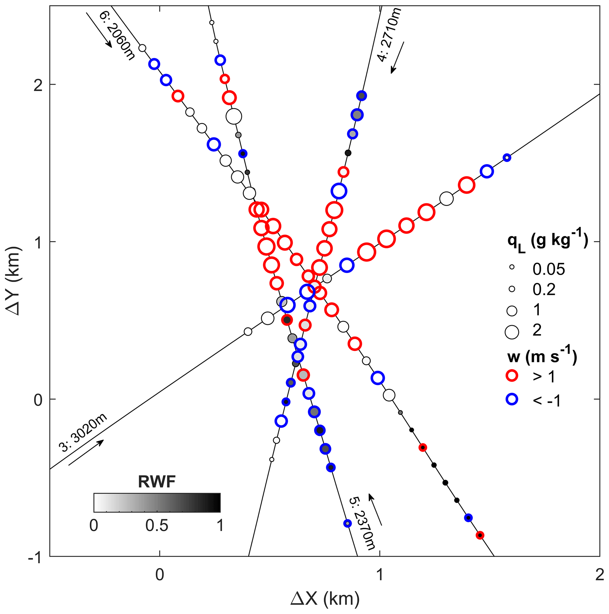
Figure 11 Four sequential Falcon in situ transects (2–3 km altitude) through a cloud during case 3. The aircraft position has been projected onto a cloud-centric coordinate where X(Y) represents the displacement along (perpendicular to) the cluster motion. The size of the markers corresponds to the total q_L, with shading indicating the rainwater fraction (RWF) defined as the fraction of q_L resulting from drop diameters exceeding 100 µm. Red (blue) rings indicate updrafts (downdrafts).

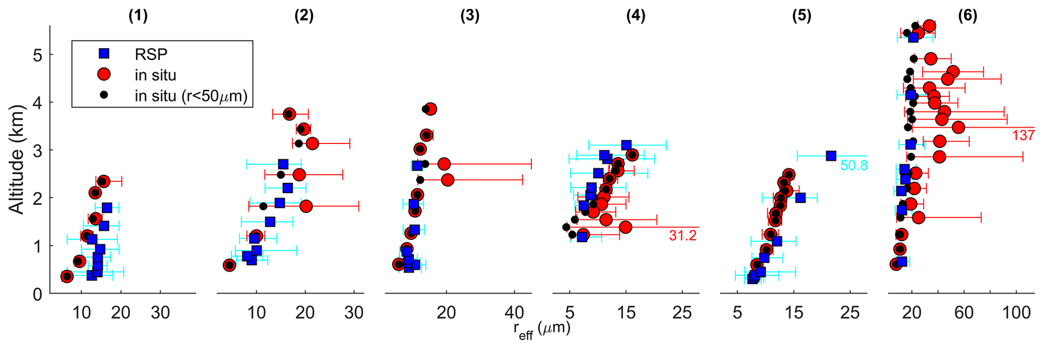
Figure 12 Comparison of the vertical profiles of effective radius, r_eff, for cases 1–6 between Falcon in situ cloud transects and composite profiles from RSP. The composite profiles were derived by grouping RSP retrievals into eight equal-frequency bins of cloud top height as determined by HSRL, with the mean altitude of each bin displayed. A comparison is made with in situ derived r_eff, omitting contributions from rainwater (r < 50 µm). For both datasets, the mean (markers) and 10 %–90 % range (bars) are shown.

A further aspect of the measurements of droplet microphysics was the availability of remote sensing retrievals to provide additional context as well as performance evaluation. Detailed analysis of the performance of combined HSRL–RSP microphysical retrievals is the topic of further study, and these cases provide unique datasets for that effort. We limit this evaluation to the retrievals of effective radius (r_eff) from RSP (note the use of radius here, by convention, while diameter is used everywhere else), which is provided at ∼ 1.2 Hz and was combined with the median HSRL-2 cloud height within each period. Statistics were determined for each case by separating the HSRL-2 cloud heights into eight equally sized subsets from which the mean and 10 %–90 % range of RSP r_eff were calculated (Fig. 12) and compared to the same statistics for each cloudy transect sampled in situ by the Falcon. RSP tended to underestimate the effective radius profile in cases where there was a dominant rain mode; this was clearly captured for case 6 where there was a closer agreement with in situ data if rainwater contributions to r_eff were omitted. There are two contributing aspects: (i) a lack of sensitivity to rain-sized drops by RSP (Alexandrov et al., 2018) that can low bias the r_eff for these cloud systems when RWF is high near cloud top and (ii) the lack of an optical signature, at RSP wavelengths, of the deep interior of the cloud where most rain-producing-drop interactions occur. Unlike the Falcon transects, which provide a statistical representation at each level (notwithstanding biases introduced from transient cloud behavior), the RSP statistics reflect the microphysics of the outer “crust” of the cloud cluster.

5.6 Sub-cloud precipitation

Rain rates were determined during in situ sampling legs carried out below cloud base to estimate the significance of surface precipitation. In the absence of radar data, it is challenging to place the under-sampled aircraft data into a statistical context; therefore the reported precipitation reflects only a snapshot and may contain biases associated with the flight strategy. The upper size limit of the 2D-S (1.5 mm) also under-sizes the contribution from large rain drops, which may cause a low bias in calculated rain rates. Considering these caveats, evaluation of sub-cloud precipitation was more focused on the relative differences between cases than on assessing the broader relevance of rain rate absolute values.

Maximum (90 %) and mean rain intensities (Table 2) were calculated from DSD data for each sub-cloud altitude using a threshold precipitation rate exceeding 0.01 mm h⁻¹ to define rainy regions. The spatial distribution of precipitation tended to be highly concentrated in visually identifiable rain shafts, and the flight line was adjusted to fly through their (visual) center when possible. In cases where multiple sub-cloud altitudes were flown, the leg with the highest rain coverage and rain intensity was retained. No sub-cloud precipitation was encountered during case 1 or 5A, and in cases 5B and 3, the rain was concentrated in a single narrow region less than 1 km in horizontal extent. To the extent that was possible, camera imagery was used to confirm that no major region of precipitation was missed simply by the choice of flight track. Case 5B was unusual because the maximum rain intensity was comparatively high (3.87 mm h⁻¹), but it was limited to a very narrow region (0.6 km) in an otherwise completely non-precipitating cloud line. Conclusions drawn from comparing the maximum or mean rain intensity were similar, and, as a singular metric for identifying the significance of precipitation in each case, the mean rain intensity did not capture the extent of the rainy region and therefore would over emphasize precipitation in cases 3 and 5. Conversely, the transect mean (not included) was heavily biased to the sampling details of each particular case (e.g., the time spent sampling the clear-sky region). With a desire to derive a characteristic rain rate comparable amongst cases, the fractional rain coverage was estimated as the ratio between (linear distance) rain coverage below cloud and the maximum horizontal linear extent of Falcon cloud sampling aloft at any altitude. The product of the fractional rain coverage and mean rain intensity provided a cluster rain rate (Table 2). While an area fraction would be a more desirable quantity by which to derive this measure, the aircraft sampling tended to align with a principal cloud axis and therefore provided limited information by which to assess a second spatial dimension, and any assumptions would need to be case specific. Using the derived cluster rain rate, cases ranged from non-precipitating (1 and 5A) to a maximum for case 4, which interestingly revealed similar rates for 4A (0.45 mm h⁻¹) and 4B (0.52 mm h⁻¹) despite their differing convective characteristics, maturity, and peak rain intensities.

6 Composition

6.1 Trace gases

In situ bulk statistics (Table 2) and vertical profiles (Fig. 13) of CO, CO₂, CH₄, and O₃ were derived for each case. Vertical profiles were separated into data collected during cloud penetrations (in-cloud), adjacent cloud-free regions sampled between each cloud level (near-field), legs below cloud base (sub-cloud), and the spiral profile (far-field). Differences between the near- and far-field data reflect the influence of the cloud system on the vertical structure of the environment in combination with pre-existing horizontal gradients. Differences between the in-cloud and near-field data are caused by convective transport. For CO, the statistical significance of profile differences was reduced because the magnitudes of the CO variations were proportionally smaller compared to the instrument precision (5 ppb_v, 0.4 Hz).

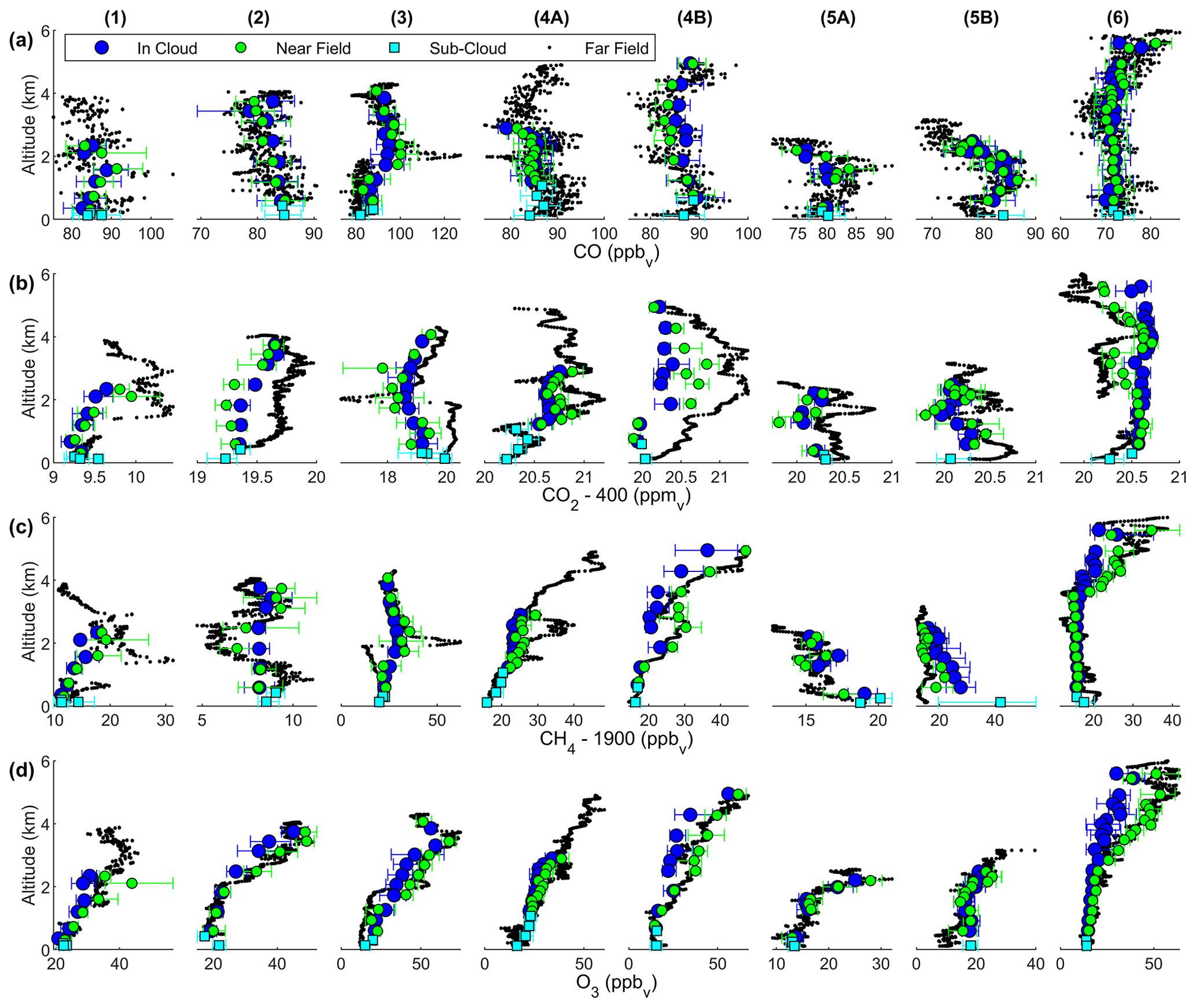
Figure 13 Trace gas vertical profiles separated into a far-field component measured during the Falcon clear spiral (black), a near-field component measured outside but in the vicinity of the cloud cluster at cloudy altitudes (green), an in-cloud component (blue), and a sub-cloud component (cyan). Data are shown for cases 1–6 for (a) CO, (b) CO₂, (c) CH₄, and (d) O₃. Note the changes in concentration scales.

Near- and far-field profiles were generally similar across cases except for case 3. Near-field CH₄ and O₃ most closely tracked trends associated with the far-field vertical structure but tended to filter smaller-scale features, perhaps indicating the influence of convective mixing on the near-field environment. This was generally more noticeable in the case of CO₂, where far-field overall vertical gradients were less apparent. In case 3, the far-field profile was characterized by a significant vertical gradient at 1.8–2.0 km where CO, CH₄, and O₃ rapidly increased (45, 50, and 35 ppb_v, respectively), while CO₂ decreased (4 ppm_v). Above this altitude, O₃ continued to increase while the trend in other species reversed. This pattern was a result of an air mass of marine origin undercutting a continental air mass aloft that had the signatures of anthropogenic influence coupled with a reduced CO₂ background caused by summertime biogenic uptake. The location of case 3 on the gradient between polluted and background air masses meant that the near-field and in-cloud concentrations were affected by both vertical and horizontal mixing.

In-cloud concentrations generally exhibited a smaller dynamic range, in line with expectations that cumulus serves to transport sub-cloud air upwards and vertically homogenize near-field environmental air through entrainment, and hence their concentrations reflected a weighted average of sub-cloud and near-field properties. In most cases there were many combinations of “weights” that could explain the in-cloud concentrations, but in some cases it is possible to do so while restricting contributions to the same level and below. Such scenarios are necessary for the archetypal rising entraining plume model of cumulus, such that in-cloud concentrations lag behind vertical gradients in the environment. However, there were identifiable cases where the in-cloud concentrations led the environmental gradient, such as O₃ and CH₄ in case 3 and CO₂ in case 2 and (marginally) case 6. These cases required air from higher altitudes to explain the in-cloud concentrations and hence suggest that simplified descriptions of lateral entrainment in shallow cumulus (e.g., de Rooy et al., 2013) should also account for (i) laterally entraining cloudy downdrafts, which were ubiquitous in all these cases (Fig. 7), and (ii) the temporal characteristic of thermal bubbles. Further development and testing of theory and models for cumulus entrainment and detrainment is not the focus here, but these case studies provide comprehensive datasets on which to base such an effort.

6.2 Aerosols

Aerosol optical property typing provided by HSRL-2 (Burton et al., 2014) indicated the fractional contributions of aerosol types (classified as marine, polluted marine, urban, smoke, fresh smoke, dust, and dusty mix) by altitude during the entire King Air module (Fig. 14a). The “unclassified” type represents mixes or a lack of typeable signatures, while the remaining absent fraction was not typeable because of a lack of aerosol scattering, obscuration by cloud, or missing lidar data. A primary signature of marine aerosols was observed for cases 1–3, with a secondary contribution from continental sources typed mostly as smoke influencing layers between 1 and 2.5 km (particularly in case 3). Cases 5 and 6 indicated a dominant dust layer, with the influence of marine aerosols taking a secondary role confined to the lowest 500 m. The dust was assumed to be of Saharan origin based on back trajectories, and it persisted during other ACTIVATE flights during this time period (i.e., flights that were not process studies). Long-range transport of Saharan dust has been shown to inhibit cloud growth in this region (Gutleben et al., 2019) and may partially explain some of the characteristics here (e.g., the differences between case 5A and case 5B). The smoke classification and particularly the identification of fresh smoke during case 4 was inconsistent and difficult to reconcile because of the absence of candidate sources and other signatures that are expected for smoke, such as elevated sub-micrometer organic aerosol mass (Fig. 14c) and CO (Fig. 13a). The back trajectory and the consistent synoptic pattern across the 5 d that included cases 4–6 would create an expectation for case 4 to share the dust classification of cases 5 and 6, and indeed aerosols were typed as dusty mix during part of the statistical survey flight on the morning of 10 June (not shown). Both dust and smoke are depolarizing, and it is possible that a misclassification could result from a dusty mix that is more aged, perhaps more coated with secondary aerosol, and contains a higher (optical) influence from accumulation mode particles (of any source) that decreases the particle depolarization and increases the lidar ratio.

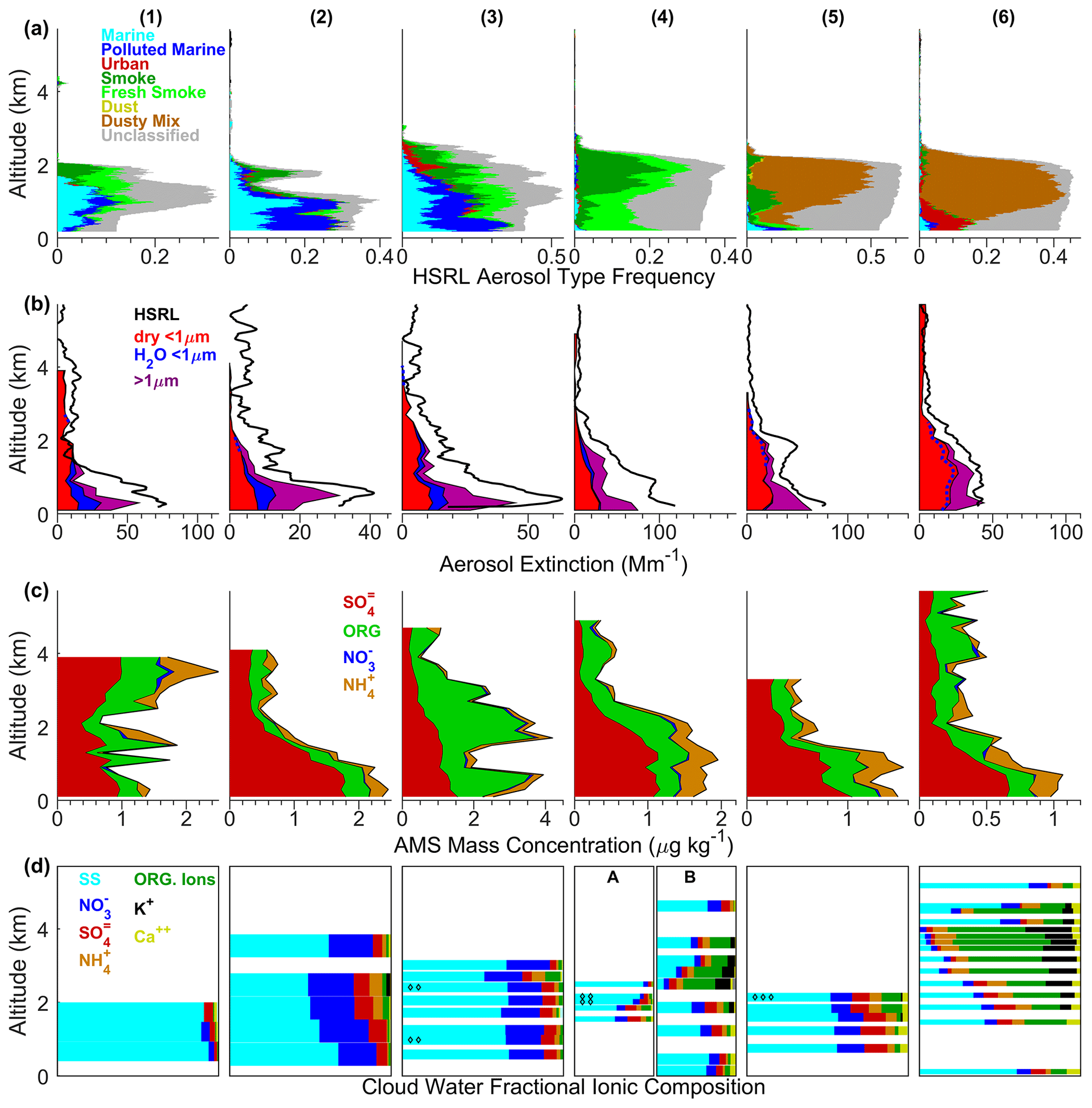
Figure 14 Vertical profiles of aerosol and cloud composition. (a) Aerosol type frequency as derived by HSRL, (b) aerosol extinction components and comparison with HSRL, (c) aerosol sub-micrometer mass measured by the AMS, and (d) ionic composition of cloud water (note that no samples were captured during case 5A, and repeated samples at the same level are marked).

Aerosol extinction from HSRL was mostly confined to the lowest 2 km of the atmosphere (Fig. 14b), with cases 1–3 indicating a more prominent enhancement in the lowest 1 km. With a deeper marine mixed layer than in other cases, case 2 exhibited the characteristic signature of aerosol hygroscopic growth leading to a defined maximum in extinction near the top of the mixed layer: a pattern also seen in cases 1 and 3 but associated with a layer that was shallower. In situ sub-micrometer dry extinction was computed from the sum of particle absorption and nephelometer total scattering measured at two relative humidity (RH) levels and was scaled to RH = 20 % using a gamma hygroscopic growth model. The contribution from sub-micrometer aerosol water was estimated by determining the sub-micrometer extinction at the ambient RH and subtracting the dry component. The super-micrometer extinction was estimated from particle area derived from the FCDP particle size distribution (assumed to represent ambient RH) and an extinction efficiency calculated from the Mie theory, assuming a refractive index for water (1.33±0i). Overall, the in situ components of the ambient extinction capture the shape of the HSRL profile, but the HSRL profile is generally enhanced in overall magnitude by between 21 % (case 6) and 77% (case 3). In cases 1–3, aerosol water contributed between 36 % and 47 % of the dry extinction to the total sub-micrometer budget within the lowest 1 km, which spanned the mixed layer and the lowest part of the layer occupied by cumulus. It is expected that water would contribute a similar or larger component to the super-micrometer extinction for these cases, based on the expectation of sea spray dominance. Both in situ and HSRL data were screened to remove clouds, but both respective methods have unavoidable differences. In addition, the relationship between aerosol water, humidity between 90 %, and saturation is strongly convex, meaning that contributions from air parcels near saturation have a highly disproportionate role and could easily explain the differences seen at low altitude in cases 1–3. Aerosol water contributed minimally to sub-micrometer extinction in cases 4–6, consistent with the expectation of dust. The super-micrometer extinction estimates are likely to be more uncertain in these cases because (a) the sizing obtained from the FCDP was derived from an assumption of spherical water droplets, and (b) particles between 1 µm dry diameter and the smallest-observable FCDP diameter at ambient humidity would be under-reported.

Non-refractory sub-micrometer particle composition (Fig. 14c) was dominated by sulfate in all cases, except case 3 where some layers were more organic dominant in alignment with a greater influence of continental pollution. While the organic contribution for other cases was too small to further interrogate the characteristics, the case-3 organic aerosol indicated a lower degree of oxidation, as quantified by the f₄₄ AMS mass fraction, in the region below 1 km (0.10) compared to the 1.5–2.5 km range (0.15). The mass ratio of ammonium to sulfate did not have an observable vertical change and ranged from 0.12 to 0.27, with case 1 and 2 less neutralized than ammonium bisulfate, case 3 approximately equal to ammonium bisulfate, and cases 4–6 lying between bisulfate and fully neutralized ammonium sulfate.

6.3 Cloud drop composition

Cloud water composition (Fig. 14d) was strongly influenced by sea salt, assumed to be a direct consequence of cumulus clouds lofting air from the marine mixed layer below cloud base and in broad agreement with other recent cloud water measurements of vertically developed cumulus (Crosbie et al., 2022; Stahl et al., 2021). The largest component of cloud water ionic mass can be attributed to sea salt in cases 1–3 at all altitudes (89 %–94 %, 49 %–67 %, and 51 %–66 %, respectively) and is also in support of the increased prevalence of HSRL marine aerosol types below cloud (Fig. 14a). The emergence of nitrate in the cloud water composition of cases 2 and 3 (24 %–31 % and 12 %–27 %, respectively) occurs with an increase in the polluted marine designation by HSRL, perhaps confirming additional influence of anthropogenic sources compared to case 1. Non-sea-salt sulfate (4 %–8 %) and organic ions (1 %–9 %) were proportionally enhanced during case 3, also supporting continental pollution influence. Non-sea-salt calcium, a common tracer for dust, was more enhanced in cases 4–6 (0.9 %–9 %) than in 1–3 (0 %–2 %), and, interestingly, this was also accompanied by an increase in non-sea-salt potassium in the middle and upper regions, particularly for case 6, that contributed up to 20 % by mass. Dust contains a greater fraction of insoluble material that does not contribute to the analysis of cloud water ions. Case 4 and case 6 also exhibit larger vertical changes in the cloud water composition, and that is notable because these cases were deepest and most affected by precipitation, potentially providing a mechanism for increased vertical stratification in drop composition. Enhanced sea salt in energetic cumulus tops has been observed elsewhere (e.g., Crosbie et al., 2022) and featured here mainly in cases 2, 4B, and 6. Notably though, clean regions at higher altitudes and the influence of precipitation removal on solutes may partly explain enhanced variability in relative composition, as small perturbations can generate large influences. Nonetheless, consistency across several sequential data points adds to the robustness of the observed trends.

7 CCN Activation and aerosol microphysics

7.1 Sub-cloud aerosol

In situ aerosol particle size distributions were compiled for the sub-cloud environment in each case and normalized to unit integrals (Fig. 15a), showing the merged contributions from the SMPS and LAS. Across all cases the distributions reveal a clear multimodal structure, with dominant contributions from Aitken and accumulation modes separated by well-defined minima (Hoppel et al., 1986), except in case 3 where the Aitken mode is broader and slightly larger. The less pronounced Hoppel minimum found in case 3 is aligned with expectations for enhanced influence from continental pollution (see Sect. 6), which may have undergone proportionally less cloud processing.

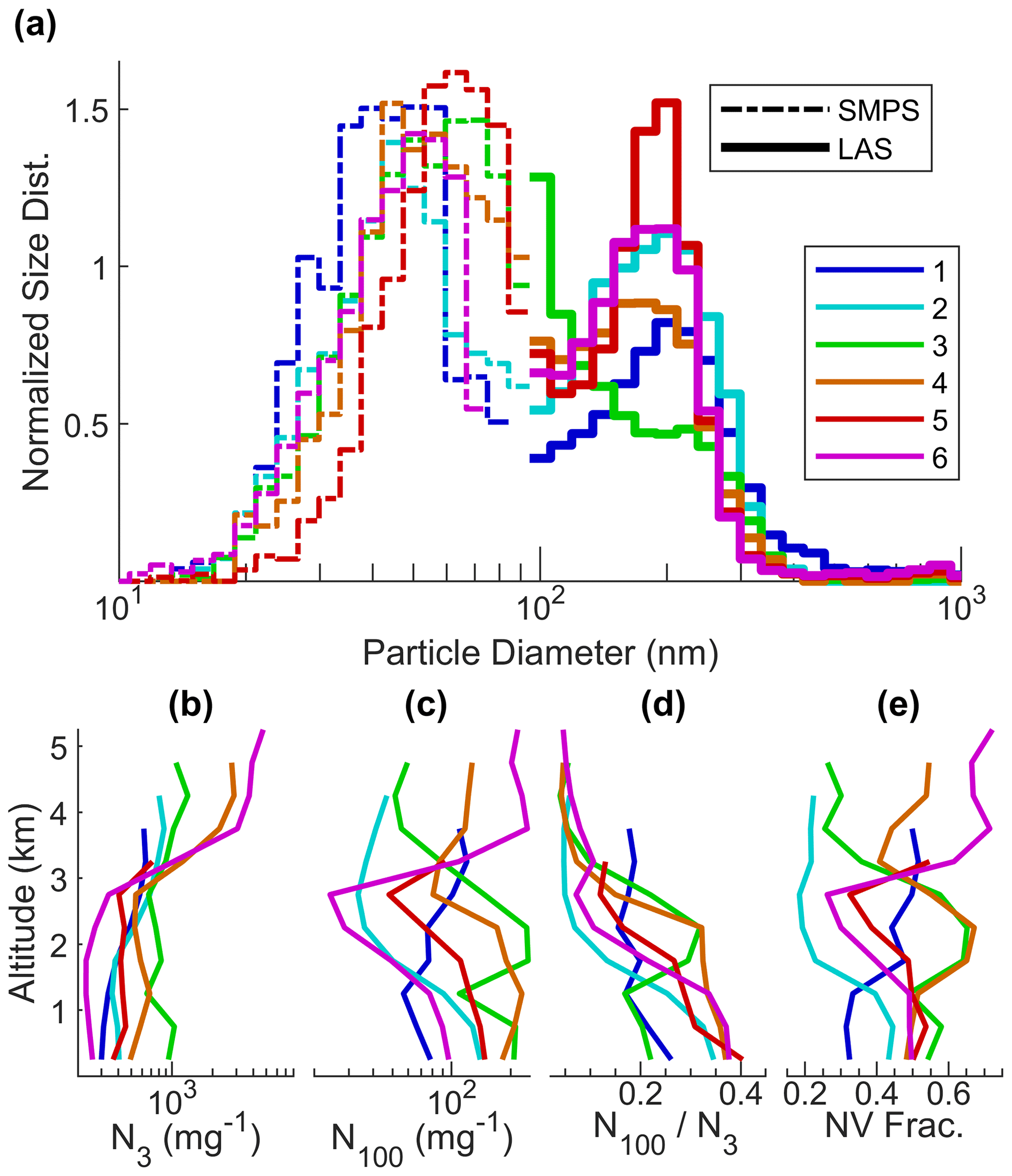
Figure 15 Aerosol microphysical properties for each case. (a) Normalized particle size distributions in the sub-cloud region and profiles of (b) total particle number concentration (> 3 nm), (c) total particle number concentration (> 100 nm), (d) the number fraction > 100 nm, and (e) non-volatile number fraction (> 10 nm).

Contributions to each mode are fitted to log-normal distributions, and parameters are provided in Table 2. Across cases, the Aitken mode varied from 43 to 64 nm, while the accumulation mode varied from 180 to 230 nm. An activation diameter was estimated as the size above which the integrated number concentration would equal the estimated N₀ (Table 2) and ranges from 52 to 74 nm. CCN counter data at 0.37 % supersaturation are included in Table 2, but closure of these data to the particle size distributions would require unrealistically high particle hygroscopicity for cases 4–6 based on equilibrium drop activation calculations (not shown). In lieu of a detailed droplet closure analysis, the LAS number concentration (> 100 nm), N₁₀₀, is quite effective at predicting N_d0 using a constant scaling factor of 1.84 and explains 80 % of the variance in N_d0 amongst these cases.

7.2 Vertical profiles

Total particle number concentration data are block averaged in altitude bins of 500 m across all cloud-free regions to capture the vertical structure of the environment as sampled in situ by the Falcon. Figure 15 (panels b and c) shows the profile of total particle number concentration (> 3 nm, N₃) and N₁₀₀, as well as their ratio (panel d) and the non-volatile fraction, NVF (> 10 nm, panel e).

N₃ generally decreased or remained constant through the lowest 2 km and then increased above 3 km. This upward trend is most apparent for the three cases conducted in 2022 in Bermuda (cases 4–6), where a marked transition to higher concentrations was observed and was also observed to occur for larger particles (> 100 nm). In cases 4 and 6, increasing N₃ with altitude above 3 km was correlated with enhancements in CO and CH₄ (Fig. 13) and with minor increases in particle organic mass (Fig. 14c), suggesting continental origin. While the beginnings of the uptick in particle concentrations were consistent for case 5, correlations were not discernible because the vertical extent of the sampling was truncated in line with the vertical extent of the cloud cluster. The close vertical alignment of the increase in N₃ and N₁₀₀ in the environment (Fig. 15) with the inflection in the profile of N_d for cases 4B and 6 (Fig. 7c) is perhaps an additional indication of the secondary activation of entrained CCN. Case 6 offers a favorable dataset to evaluate entrained activation (e.g., in parcel models and LES) because of the sharpness of the aerosol gradient and the abundance of larger (N₁₀₀) particles aloft. In contrast, cases 2 and 3 show markedly reduced N₁₀₀ above 3 km, with a major distinction between these two cases occurring between 2 and 3 km as a result of the organic-rich pollution layer affecting case 3.

Across all cases the fraction of larger particles decreases with altitude (Fig. 15d), with the ratio $N_{\mathrm{100}}/N_{\mathrm{3}}$ varying from 22 % to 40 % in the lowest-altitude bin to less than 6 % above 4 km (for the cases where data were available). NVF provides an indicator for refractory cores enhanced in layers enriched in primary combustion particles as well as dust and sea spray, while low values typically indicate an abundance of (nucleated) secondary aerosol species. At low altitudes, the marine-dominated cases 1 and 2 had the lowest NVF (32 % and 42 %, respectively), which is supportive of a large number fraction of marine particles originating from new particle formation and subsequent secondary aerosol growth, with the pollution-influenced case 3 being the highest (54 %) and the Bermuda 2022 cases 4–6 tightly clustered between 48 % and 50 %. Near 2 km, the influence of continental pollution is most significant in case 3, as determined by the organic enrichment (Fig. 14c), and is accompanied by higher NVF, while case 2 relaxes to an unperturbed free-tropospheric background with low aerosol mass, smaller particles, and the lowest NVF. It is notable that in the purportedly dust-influenced layer at 1.5–2.5 km in cases 4–6, there is a distinct difference in NVF between case 4 (which mimics the enhancements of case 3) and cases 5 and 6 (which instead decrease) that may provide further insight into the optical signature leading to the smoke classification of case 4 (Fig. 13a).

8 Discussion and conclusions

This measurement report describes six case studies relating to airborne observations of aggregated regions of marine shallow cumulus and cumulus congestus. The observations incorporate a coordinated flight strategy centered on a target cloud cluster and involved a HU-25 Falcon that sampled the cloud and surrounding environment in situ, while a King Air made repeated remote sensing passes above the scene, dropping dropsondes around the perimeter and near the center.

The large-scale meteorology was broadly consistent across cases, with a subtropical anticyclone located to the east resulting in northward advection of moist tropical air masses, and the planetary boundary layer (PBL) air mass origin (8 d) was the trade wind region of the central tropical Atlantic. As the low-level air masses advected around the southwest quadrant of the subtropical high moving northward into the subtropical region, mid-tropospheric temperatures decreased, while SSTs remained close to tropical levels, typical of the summertime western Atlantic. Three of the cases were conducted over the warm Gulf Stream waters near the United States east coast, while the other three occurred over relatively uniform SST near Bermuda. The warm, moist advection and surface fluxes maintained the PBL thermodynamic properties close to tropical conditions, while the reduction in mid-tropospheric temperature may explain the destabilization of the profile, permitting nearby deeper convection, and the lack of a defined capping inversion for most of the cases.

Overall, there was not a strong association between localized increases in static stability and the frequency of cloud top observations at that altitude. This may indicate that the environmental moisture profile, wind shear, cloud horizontal scale, and perhaps microphysics all contribute to the vertical distribution of cloud heights in situations where a strong capping layer is absent. Also notable was the lack of a universal relationship amongst the cluster motion vector, the shear vector, and the principal linear axis of organization, which is perhaps indicative of a memory effect that sustains a favored orientation after formation.

Multiple passes through the cloud clusters revealed considerable variability in the cloud system properties compared to an idealized adiabatic parcel and confirmed the ubiquity of environmental entrainment in affecting the bulk characteristics. Evidence of transient thermals was observed through the variability in the spatial distribution of vertical velocity, bulk water content, and microphysical properties between sequential transects. Downdrafts were commonly observed, often near cloud edges, and there were some, albeit limited, examples where gas tracer concentrations within the cloud could only be explained by incorporating environmental air from a higher altitude. In some cases, cyclical collapse of emergent convective turrets resulted in net downward transport of cloud water near cloud top. These cases offer a unique dataset to evaluate and improve convective parameterization of entrainment and detrainment for shallow cumulus.

The effect of entrainment on generating sub-adiabatic q_L was less impactful on N_d and was found to be generally consistent across cases. This was not associated with a uniformly reduced droplet growth rate (as might be anticipated with homogeneous mixing) but rather with a source of N_d from activation of entrained air that manifested as a distinct mode of small droplets in the DSD occurring alongside a mode that grew close to the (monodisperse) adiabatic rate. The result was a broadening of the DSD with altitude, as quantified by the relative dispersion. Further analysis and parcel modeling are needed to fully explore this concept in detail, but an underpinning factor is that the timescale for entrained air (e.g., at the eddy scale of thermals) to homogenize within a cloudy volume is slow compared to the time taken for the entrained air to be carried upwards to its particular LCL. Further evidence that pointed towards the activation of entrained air was found in two cases where N_d transitioned to an increase with altitude above 3 km in concert with an increase in the number of CCN-active particles in the environment.

Precipitation below cloud base was spatially concentrated into narrow regions and in some cases was absent or negligible. It was found in at least one case that rainwater formed near cloud top was expelled laterally by subsequent thermals, where much of the rainwater was anticipated to ultimately evaporate into the dry surrounding environment, explaining the limited extent of precipitation at lower altitudes. The cases which exhibited the highest near-surface precipitation were associated with markedly different frequency distributions of cloud top altitude, perhaps indicating a threshold above which the precipitation substantially influences the cloud dynamics. The remaining cases would tend to indicate that precipitation is a consequence and not a cause of aggregation and deepening.

Across the cases, shared attributes may provide useful means to isolate specific mechanisms or modes for further investigation. These are summarized by the following points.

• Cases 1 and 5 were the least vertically developed and both exhibited pronounced linear organization with either very isolated or no observed precipitation below cloud base. Cloud motion was slightly (8 and 15°, respectively) to the left of the axis of cloud organization with veering of the wind (i.e., clockwise rotation) with altitude, such that the cloud-top-to-base shear vector was approximately perpendicular to the cloud axis and remarkably similar in magnitude. Different features for case 1 included steering winds being stronger by a factor of ∼ 2, being located over the Gulf Stream (rather than near Bermuda), and that the aerosol was indicative of background marine conditions, while case 5 was influenced by Saharan dust. Case 5 incorporated observations of two systems: 5A, which was decaying, and 5B, which was active, with 5A more influenced by the Saharan dust.

• Cases 2 and 3 exhibited intermediate levels of vertical development with a clear distinction between the vertically developed cluster and the surrounding boundary layer cumulus, and both showed evidence of clearings forming in the immediate surroundings (more notable in case 2). Both cases were located over the Gulf Stream. Case 3 was more influenced by continental pollution leading to higher N_d. Convective vertical velocity extrema were stronger in case 3, perhaps indicating a liquid-phase microphysical invigoration mechanism, while precipitation was more influential in case 2. A notable difference in the organization was in the orientation of the cloud axis, which was parallel to the cluster motion in case 2 and perpendicular in case 3.

• Cases 4 and 6 were cumulus congestus cases and the most vertically developed. The vertical distributions of cloud cover were different from the other cases, with the emergence of detrained layers in the environment surrounding the convection. These cases also captured a distinct lifecycle, with the cloud cluster apparently deepening too rapidly to sustain itself. This was captured in the measurements of case 4A, which sampled the remnants of a previously deeper system, and in case 6, where the cloud system ceased to exist shortly after the sampling was completed. These cases offer unique datasets for detailed analysis of the convective lifecycle of cloud clusters.

In conclusion, this measurement report documents a novel strategy of utilizing two coordinated aircraft to conduct in situ and remote sensing observations of aggregated shallow cumulus and cumulus congestus during the NASA EVS-3 ACTIVATE summer field campaigns spanning 2020-2022. Six process study cases have been reported, providing the background and supporting information associated with the measurements to guide further analysis and modeling. The datasets collected during ACTIVATE provide a unique and comprehensive characterization of dynamic, thermodynamic, trace gas, aerosol, and cloud properties at a high temporal resolution, and the implementation of this flight strategy provides targeted observations of individual cloud clusters and their environments.