Significant impact of urban tree biogenic emissions on air quality estimated by a bottom-up inventory and chemistry transport modeling

Biogenic volatile organic compounds (BVOCs) are emitted by vegetation and react with other compounds to form ozone and secondary organic matter (OM). In regional air quality models, biogenic emissions are often calculated using a plant functional type approach, which depends on the land use category. However, over cities, the land use is urban, so trees and their emissions are not represented. Here, we develop a bottom-up inventory of urban tree biogenic emissions in which the location of trees and their characteristics are derived from the tree database of the Paris city combined with allometric equations. Biogenic emissions are then computed for each tree based on their leaf dry biomass, tree-species-dependent emission factors, and activity factors representing the effects of light and temperature. Emissions are integrated in WRF-CHIMERE air quality simulations performed over June–July 2022. Over Paris city, the urban tree emissions have a significant impact on OM, inducing an average increase in the OM of about 5 %, reaching 14 % locally during the heatwaves. Ozone concentrations increase by 1.0 % on average and by 2.4 % during heatwaves, with a local increase of up to 6 %. The concentration increase remains spatially localized over Paris, extending to the Paris suburbs in the case of ozone during heatwaves. The inclusion of urban tree emissions improves the estimation of OM concentrations compared to in situ measurements, but they are still underestimated as trees are still missing from the inventory. OM concentrations are sensitive to terpene emissions, highlighting the importance of favoring urban tree species with low-terpene emissions.

1 Introduction

With an increasing number of people living in cities, urban areas are experiencing continuous expansion (Angel et al., 2011; United Nations, 2018). Artificial surfaces with darker, impermeable materials and high buildings, as well as release of anthropogenic heat, strongly modify the energy budget of the urban area (Taha et al., 1988; Taha, 1997; Pigeon et al., 2007a; Kuttler, 2008; Oke et al., 2017; Masson et al., 2020). An increase in temperature in the city compared to the surrounding countryside is often observed and is called the urban heat island (UHI) effect (Oke, 1982; Kim, 1992). Due to the high local emission sources (traffic) and the modification of airflows by tall buildings which limits the pollutant dispersion, concentrations of several pollutants, such as NO₂ and particles, are higher in cities than the surrounding areas (Lyons et al., 1990; Fenger, 1999; Thunis, 2018; Li et al., 2019; Yang et al., 2020).

To mitigate the negative effects of urbanization, urban vegetation and trees in particular are now widely promoted (Livesley et al., 2016; Chang et al., 2017; Roeland et al., 2019). Trees can locally reduce air and surface temperatures by creating shade and by evaporating water through transpiration (Jamei et al., 2016; Taleghani, 2018; Lai et al., 2019; Hami et al., 2019; Nasrollahi et  al., 2020). Trees can also remove gaseous and particulate pollutants from the atmosphere by dry deposition, although this effect is quantitatively questionable due to the large variability and uncertainties (Nowak et al., 2006; Escobedo and Nowak, 2009; Setälä et al., 2013; Selmi et al., 2016; Nemitz et al., 2020; Lindén et al., 2023).

Trees are known to naturally emit biogenic volatile organic compounds (BVOCs). The term BVOC includes gaseous non-methane hydrocarbons and includes many families of molecules: isoprene, terpenes, alkanes, alkenes, carbonyls, alcohols, esters, ethers, and acids. BVOC emissions are involved in stress resistance mechanisms (due to heat, water shortage, oxidation, and herbivore or pathogen attack) and communication (plant–plant and plant–insect interactions) (Kesselmeier and Staudt, 1999). Emission rates depend on abiotic factors such as temperature and light, and biotic factors include things such as tree species, leaf age, and stress level (Niinemets et al., 2004; Loreto and Schnitzler, 2010; Niinemets, 2010). BVOC emissions are therefore highly variable in space and time. Unlike specific anthropogenic volatile organic compounds (AVOCs) such as benzene, emitted BVOCs may not be directly harmful to human health. However, BVOCs may form secondary pollutants, such as ozone (Calfapietra, 2013; Atkinson and Arey, 2003a; Churkina et al., 2017) and secondary organic aerosols (Salvador et al., 2020; Minguillón et al., 2016; Churkina et al., 2017; Lehtipalo et al., 2018). BVOCs emitted in the gaseous phase are oxidized in the atmosphere, forming more functionalized compounds that are semi-volatile and may be absorbed into aerosols. In the urban VOC-limited environment with high nitrogen oxides (NO_x) (emitted by traffic), ozone formation strongly depends on the VOC concentrations. There are also feedbacks between the urban environment, which is stressful for trees (higher temperatures and concentrations of oxidizing pollutants and difficult access to water) (Lüttge and Buckeridge, 2023; Czaja et al., 2020), and BVOC emissions.

To understand processes and forecast the evolution of pollutant concentrations, numerical models are widely used. Air quality models of various types and resolutions exist, depending on the scale and processes studied. Chemistry transport models (CTMs) are Eulerian models that represent the chemistry and transport of pollutants in three-dimensional grid cells, e.g., CHIMERE (Menut et al., 2021), Polair3D (Boutahar et al., 2004), WRF-Chem (NOAA/ESRL, 2023), CMAQ (Byun and Schere, 2006; Appel et al., 2021), and MOCAGE (CNRM, 2023). Their typical horizontal resolution varies between 1 and 10² km, and they are used from the global to the regional scales (Mailler et al., 2017). Many input data are necessary: surface characterization, spatiotemporal emissions of each pollutant, and boundary and initial conditions. Due to the coarse resolution, the surface type is characterized by land use categories such as open water, urban, forest, and crop. Forest trees are usually divided into one to five categories based on general characteristics (evergreen or deciduous; broadleaf or needleleaf). Most of the CTMs compute the BVOC emissions from forest and crops based on plant functional type (PFT) and the MEGAN empirical model (Model of Emissions of Gases and Aerosols from Nature) (Guenther et al., 2006, 2012; Matthias et al., 2018). The heterogeneity of the vegetation species is not explicitly modeled, but the model gives a rough estimate of the BVOC emission rates in the grid cells containing vegetation. CTMs can be used to compute air quality over large urban areas, but at this spatial resolution, the land use is urban, and no biogenic emission from urban vegetation is taken into account. In parallel, tree inventories are being developed in many cities (Bennett, 2023) and give us a much more accurate description of the urban forest. They can contain the precise locations, species, and sizes of trees, allowing the study of the impact of urban vegetation on air quality (Mircea et al., 2023).

Based on the tree inventory implemented in Paris by the municipality (Municipality of Paris, 2023) and a series of allometric equations (McPherson et al., 2016), a method is developed to estimate the BVOC emissions by urban trees in Paris. This “bottom-up” inventory of BVOC emissions by urban trees is used to estimate emissions from Paris trees over June and July 2022. This period is chosen because biogenic emissions are expected to be higher in summer, especially during heatwaves, and also because of the numerous in situ measurements that have been performed in the Paris region. The effect on isoprene (C₅H₈), monoterpene, ozone (O₃), organic matter (OM), and particulate matter (PM) concentrations over the Île-de-France (IDF) region is quantified using the CTM CHIMERE.

2 Materials and methods

2.1 Tree-based BVOC emission model

To compute BVOC emissions in CTMs, an empirical approach is usually used. The emission rate of each BVOC species is computed as the product of several factors: the amount of vegetation (surface of the land use category and leaf area index or mass), an emission factor at the standard conditions (leaf temperature of 30 °C and photosynthetic photon flux density (PPFD) of 1000 $\mathrm{\mu }\mathrm{mol}\mathrm{photons}{\mathrm{m}}^{-\mathrm{2}}{\mathrm{s}}^{-\mathrm{1}}$), and activity factors representing physiological or meteorological effects. One emission factor is associated with each PFT. The development of BVOC rate measurements at the leaf or branch scale with chambers and tree inventories allows the estimation of BVOC emission rates at the tree level (Owen et al., 2001, 2003; Stewart et al., 2003; Karl et al., 2009; Steinbrecher et al., 2009). The emission rate of a BVOC k for a tree t (µg h⁻¹ per tree) can be estimated as

$$\begin{array}{}\text{(1)}& {\text{ER}}_{k,t}={\text{DB}}_t\cdot {\text{EF}}_{k,t}\cdot {\mathit{\gamma }}_k,\end{array}$$

where

• EF_k,t ($\mathrm{\mu }\mathrm{g}{\mathrm{g}}_{\mathrm{DW}}^{-\mathrm{1}}{\mathrm{h}}^{-\mathrm{1}}$) is the emission factor (or potential) at standard conditions;

• DB_t is the dry leaf biomass (g_DW, where DW stands for dry weight); and

• γ_k combines the different dimensionless emission activity factors.

2.2 Tree inventory and characteristics

The Paris tree database (https://opendata.paris.fr/explore/dataset/les-arbres/map/, last access: 3 March 2023) regroups an inventory of the public trees. Much mapped information is available for each tree, including the precise location (coordinates), address, type (roadside, garden, cemetery, etc.), tree species, height, trunk circumference, and development stage. It is regularly updated, and the version used in this study was downloaded in March 2023. A map of trees around Avenue des Champs-Élysées taken from the database is shown in Fig. B1. The proportion (P) of the tree genera found in Paris is presented in Fig. B2, and the distributions of their trunk circumferences and crown heights are shown in Fig. B3. The municipality of Paris estimates that around one-third of the Parisian trees are missing from their database, mainly trees located in private areas. Without further information on these private trees, they are not taken into account in this study.

To compute the BVOC emissions (Eq. 1) of each individual tree, an estimation of the leaf dry biomass is necessary. Dry biomass such as leaf area and crown dimensions can be estimated using allometric equations. These allometric relationships are statistical models based on a sample of measurements predicting tree size as a function of parameters such as trunk diameter or age since planting. Many studies propose equations for forest trees (Burton et al., 1991; Bartelink, 1997; Karlik and McKay, 2002), but studies on urban trees are more scarce (Nowak, 1996). The open database of McPherson et al. (2016) is chosen in this study because it was developed specifically for urban trees and includes many genera found in Paris (84 % of the trees in the Paris inventory) (365 growth equations for 174 tree species). For missing tree genera, an equation from another tree genus in the same family is selected, as described in Sect. 3. It includes allometric tree measurements for different climates in the United States, so assumptions are necessary to select the climate for each tree species that is the closest to that of the Paris region (see Sect. 3).

2.3 Description of regional-scale air quality simulations

To quantify the impact of the Parisian tree emissions on air quality, regional-scale simulations using the 3D CTM CHIMERE v2020_r3 (Menut et al., 2021) coupled to the chemical module SSH-aerosol v1.3 (Sartelet et al., 2020) are performed. The gas-phase chemical scheme is MELCHIOR2, modified to represent secondary organic aerosol formation, as described in Sartelet et al. (2020). Biogenic emissions are estimated using the MEGANv2.1 algorithm implemented in CHIMERE (Couvidat et al., 2018), which corresponds to a land use approach. The following section describes the simulation setup.

Simulations are performed during summer 2022, between 6 June and 31 July 2022, with a 5 d spin-up period (1–5 June). Summertime is chosen as biogenic emissions are the highest during this period due to meteorological conditions. In France, summer 2022 was exceptionally hot and sunny, with little precipitation (on average 1 to 3 °C above seasonal values over most of France) (Meteo France, 2023). The domain of study corresponds to the Île-de-France region, with a 1 km × 1 km spatial resolution (IDF1). Initial and boundary conditions are taken from two additional nesting simulations: one over France with a 9 km × 9 km spatial resolution (FRA9), and one over the northwest of France with a 3 km × 3 km spatial resolution (IDF3), as shown in Fig. 1. For the FRA9 domain, boundary and initial conditions are obtained from the CAMS platform (Inness et al., 2019), with a 10 km × 10 km spatial resolution.

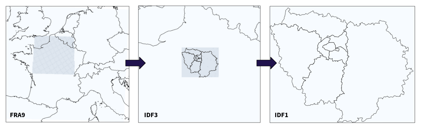
Figure 1 Representation of the simulated domains. The blue rectangles represent the location of the different nested domains.

Meteorological data for all domains are computed using the Weather Research and Forecasting (WRF) model v3.7.1 available in CHIMERE (Powers et al., 2017; Menut et al., 2021). Even if CHIMERE and WRF simulations are performed simultaneously, one-way coupling is used, and then, the concentrations computed in CHIMERE are assumed to have no influence on the meteorological fields computed by WRF. WRF simulations are performed with 33 vertical levels from 0 to 20 km altitude. A more refined vertical discretization is employed in the first four vertical levels (average heights of 0.12, 25, 50, and 83 m, respectively), which contains almost all buildings in Paris region.

The spatial distribution of each land use category used in WRF simulations is based on CORINE Land Cover (European Environment Agency, 2020)​​​​. It was chosen for its very fine resolution (250 m) since, for 1 km resolution simulations over a city, a detailed description of the land use is required to correctly describe the urban fabric. To ensure the compatibility with the Noah Land Surface Model (LSM), we converted the classification from CORINE Land Cover into MODIS (Moderate Resolution Imaging Spectroradiometer) categories, following Vogel and Afshari (2020). Three urban categories are employed to differentiate street and building dimensions, as well as heat transfer parameters in commercial, high-, and low-intensity residential areas.

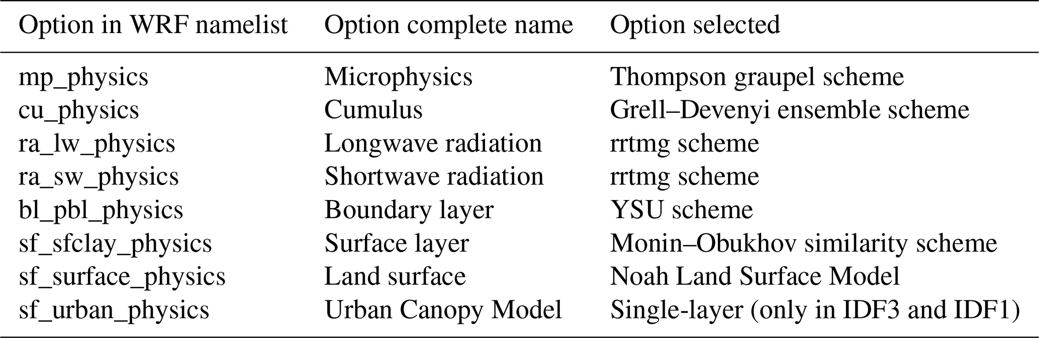
In order to represent more precisely the meteorological fields in urban areas, the single-layer Urban Canopy Model (UCM) (Kusaka et al., 2001) is used in the IDF3 and IDF1 domains. The UCM was chosen in WRF because it allows the input of anthropogenic heat (AH) fluxes for different urban categories; AH is assumed to be 45 W m⁻² for commercial areas, 10 W m⁻² for high-intensity residential areas, and 5 W m⁻² for low-intensity residential areas, based on Pigeon et al. (2007b) and Sailor et al. (2015). AH is crucial to correctly model the heat island effect, as well as the friction velocities above buildings. Table 1 summarizes the other physical options employed in the WRF simulations.

Table 1 Main physical options employed in WRF simulations.

As expected, the WRF model simulates higher temperatures in urban areas than in rural areas (fields or forests), as shown in Fig. C1, which presents the 2-month average air temperature at 2 m simulated by WRF. The simulated downwards shortwave (SW) radiation at ground surface is also used to compute tree biogenic emissions. It is quite homogeneous over the Paris region, with a 2-month average of 500 W m⁻² (daytime) and spatial variations within 5 % of the mean.

Anthropogenic emissions in the domains FRA9 and IDF3 are from the latest (2020) EMEP emission inventory (EMEP, 2019) (0.1° × 0.1 ° horizontal resolution), and in IDF1, they are from the latest (2019) regional emission inventory of the Air Quality Monitoring Network (AQMN) Airparif for the greater Paris area (https://www.airparif.asso.fr/, last access: 5 May 2024) (1 km × 1 km spatial resolution). Traffic emissions correspond to those of the summer 2022, calculated using the bottom-up traffic emissions model HEAVEN (https://www.airparif.asso.fr/heaven-emissions-du-trafic-en-temps-reel, last access: 5 May 2024), while non-traffic anthropogenic emissions correspond to the 2019 Airparif inventory.

2.4 Description of the air quality experimental measurements

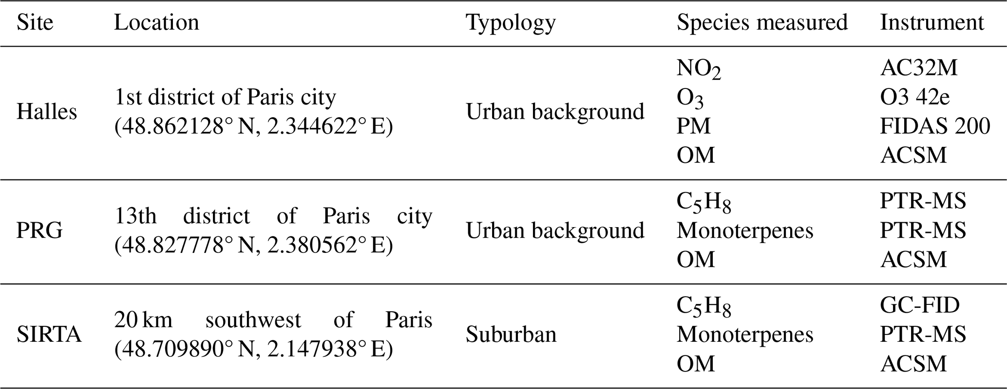
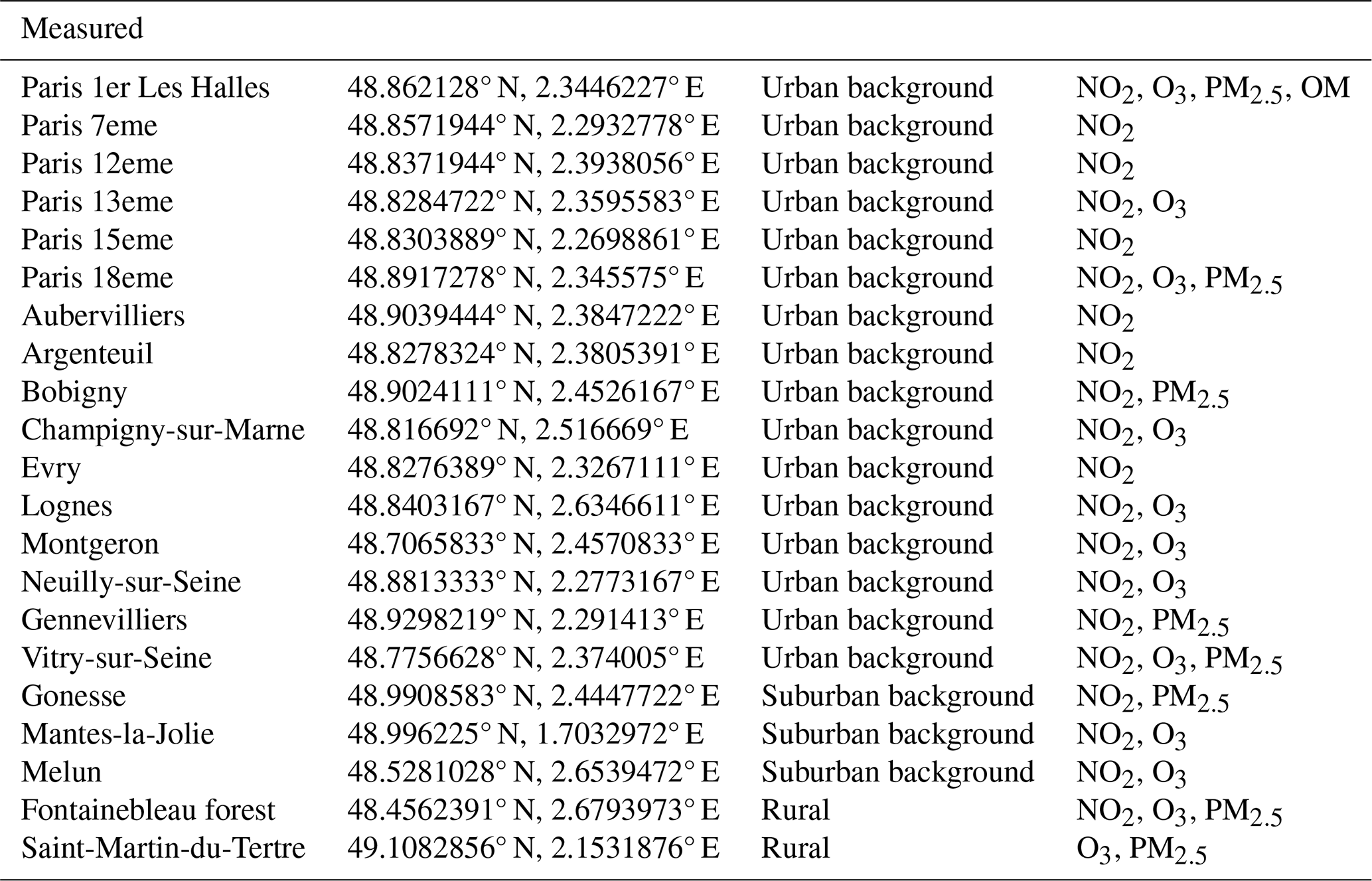
The results of the simulations are compared to experimental measurements performed at different sites in the Paris region. In Sect. 4.1.2 and 4.2, temporal variations in the observed and simulated concentrations are presented in three main sites: the Halles site, a permanent air quality monitoring station located in the city center and operated by Airparif; the PRG (Paris Rive Gauche) site, located on the seventh floor of the Lamarck B building of Université Paris Cité (30 m above ground level (a.g.l.)) in the southeastern side of the city and set up as part of the ACROSS campaign (Cantrell and Michoud, 2022); and the site of SIRTA (Site Instrumental de Recherche par Télédétection Atmosphérique), an atmospheric observatory located 20 km southwest of Paris which is integrated in the ACTRIS European Research Infrastructure Consortium (https://www.actris.eu, last access: 5 May 2024) (Haeffelin et al., 2005). The Halles and PRG stations are both urban background sites, while SIRTA is a suburban background site. The three sites and the measurements performed are described in Table 2, and a more complete description of the measurements and their associated uncertainties is provided in Appendix A.

Table 2 Description of the experimental measurements performed at different sites and used in this study. ACSM is the aerosol chemical speciation monitor (Petit et al., 2015), PTR-MS is the proton transfer reaction mass spectrometry (Simon et al., 2023), and GC-FID is the gas chromatograph with a flame ionization detector (Gros et al., 2011).

The reference simulations (without urban trees biogenic emissions) are validated in Sect. 4.1 with the observation sites of the Airparif network. These sites correspond to 21 permanent air quality monitoring stations included within a large operational stations network operated by Airparif (see Table A1 and https://www.airparif.asso.fr/carte-des-stations, last access: 5 May 2024). The map in Fig. 2 shows the location of all measurement stations which are used to evaluate the simulations (Sect. 4.1 and 4.2). It also presents the land use from GLOBCOVER (Bontemps et al., 2011) used in the CHIMERE simulation over IDF1. It is mainly composed of agricultural lands, forests of varying sizes, and a large urban area including Paris and its suburbs.

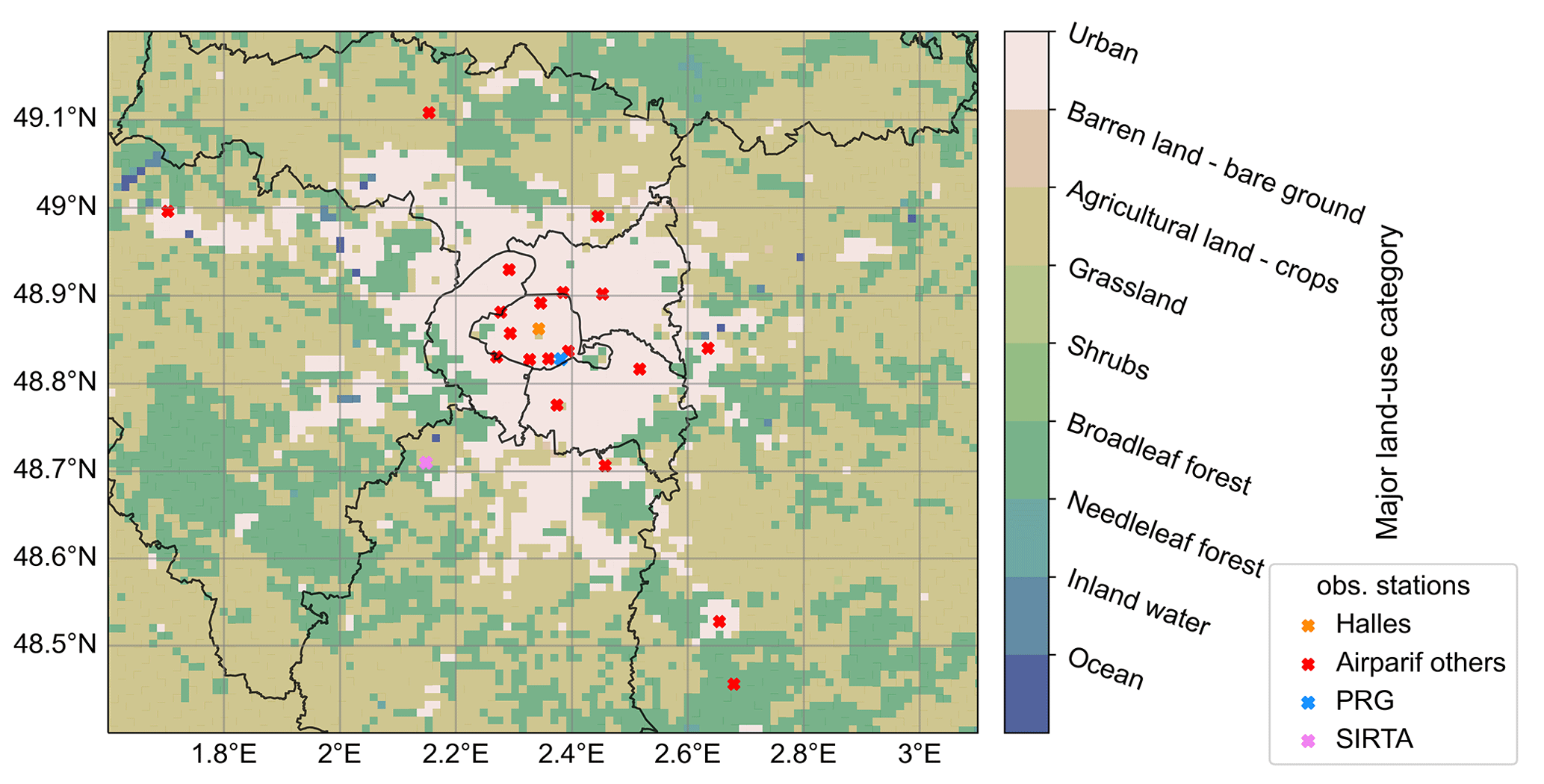
Figure 2 Map of the GLOBCOVER major land use in each grid cell used in IDF1 CHIMERE simulations. The crosses represent the locations of the different measurement stations.

3 Bottom-up inventory of tree BVOC emissions and comparison to the land use approach

3.1 Calculation of BVOC emissions at the tree level

3.1.1 Estimation of the tree dry biomass

The total tree leaf dry biomass (in grams of dry weight, g_DW) is computed based on the McPherson et al. (2016) allometric equation database. Tree data were collected in 17 reference cities representative of the different US climate zones and analyzed to obtain growth equations. The database contains equations to estimate the tree characteristics from the tree species, climate, and the trunk diameter at breast height (DBH) (at 1.3 m). To find the correspondence between Parisian trees and this database, the US climates were first ranked from closest to farthest from the Parisian climate based on a qualitative comparison of annual rainfall and temperatures (see Table D1). For each tree species in the Paris tree inventory, the allometric equations are obtained from the US database by selecting the closest tree category in terms of tree species and climate, following the decision tree shown in Fig. D1. The default species is the plane tree (Planatus × hispanica), which is the predominant species in Paris.

Then, the trunk diameter at breast height, DBH (cm), is computed from the trunk circumference, CIRC (cm), available in the Paris tree inventory for each tree, assuming a cylindrical tree trunk, as DBH = CIRC $/\mathit{\pi }$. The total tree leaf area (LA in m²) is then computed from each Parisian tree using the selected equation form and coefficient and the computed DBH. For example, the function LA =f(DBH) is shown for three tree species which have different allometric equation forms in Eqs. (D1), (D2), and (D3). Finally, the dry biomass (DB in g_DW) is the product of the leaf area and the dry weight density (DWD in g_DW m⁻²), calculated as DB_t = LA_t× DWD_t. The dry weight density depends on tree species, and it is also given in the McPherson et al. (2016) database. For instance, DWD = 500, 520, and 560 g_DW m⁻² for Planatus × hispanica, Acer platanoides, and Prunus serrulata, respectively. The computed LA and DB are shown in Fig. 3 for the predominant tree species (P> 1 %) as a function of the DBH. It shows that LA and DB increase with DBH, but there is a large variability depending on the tree species. For example, for a tree of DBH = 100 cm, the estimation of the leaf surface is equal to 1151.5 m² for Planatus × hispanica, 582.5 m² for Acer platanoides, and 1147.7 m² for Prunus serrulata.

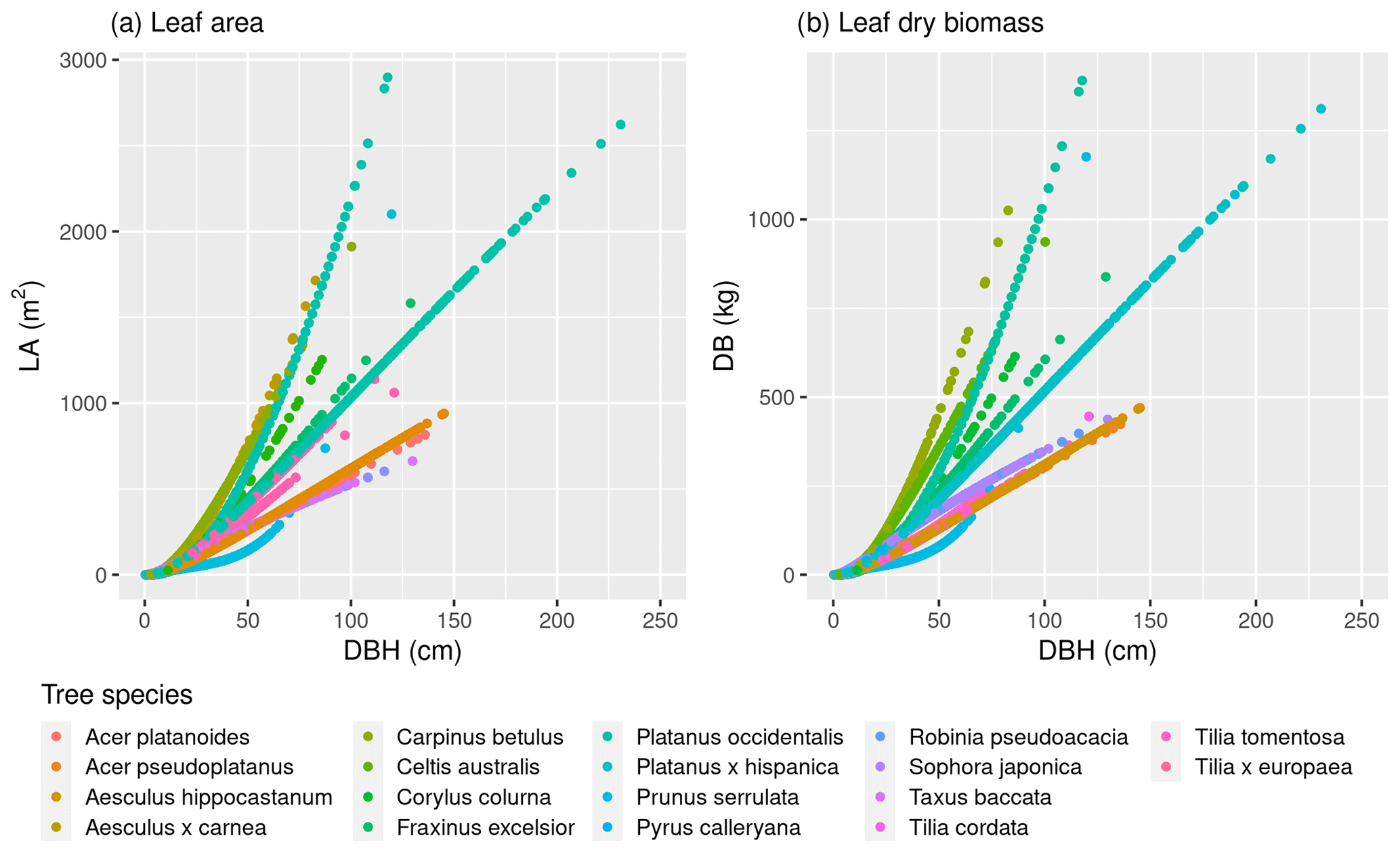
Figure 3 (a) Leaf area (LA) and (b) dry biomass (DB) computed for the predominant tree species (P> 1 %) in the Paris city inventory as a function of DBH.

As the simulation is performed during the late spring and summer periods, the tree foliage is assumed to be fully developed, so that the leaf area and dry biomass are constant over time. For longer simulation periods, the temporal evolution of leaf area and dry biomass should be introduced.

3.1.2 Emission factors by tree species and computation of activity factors

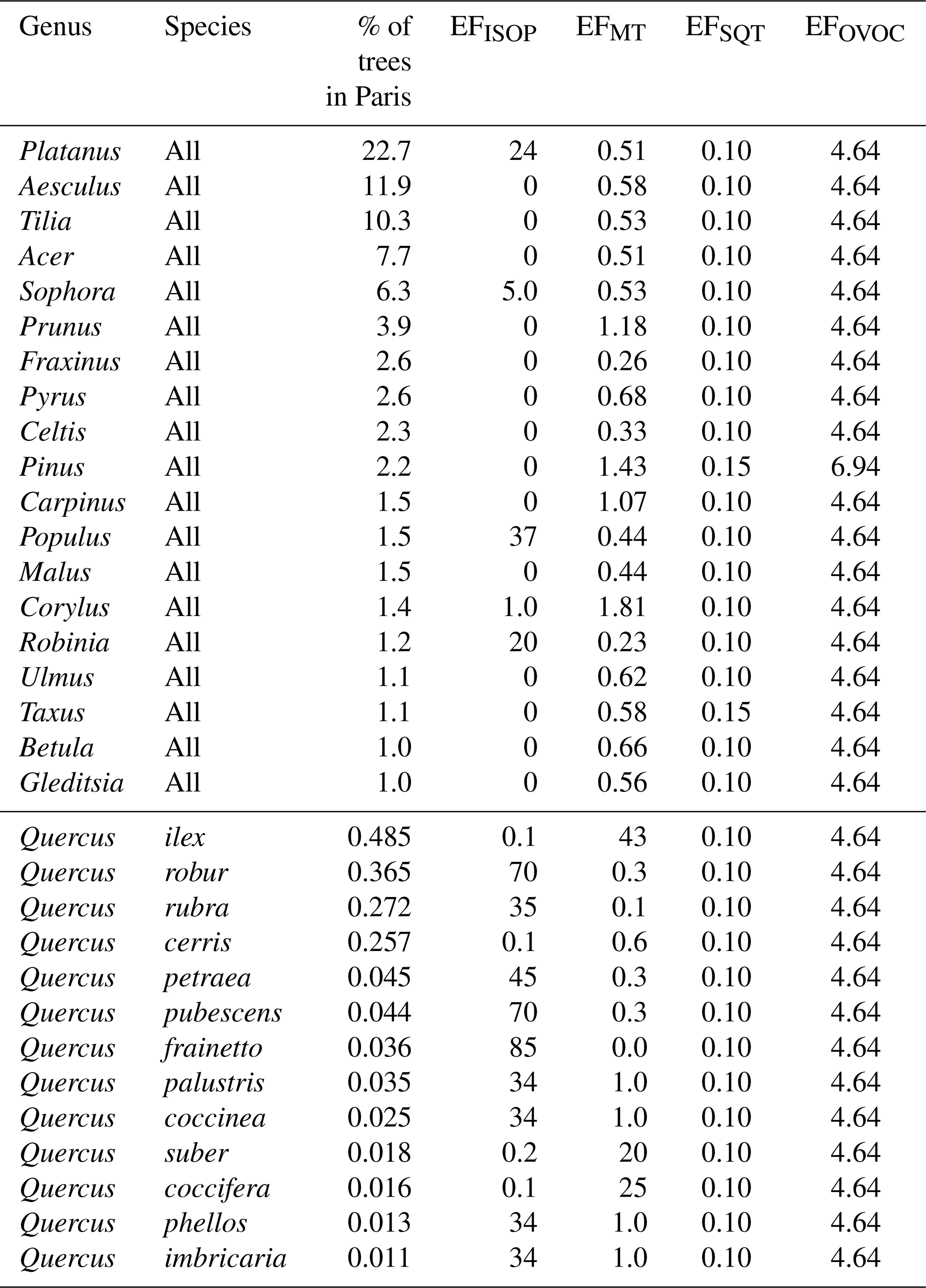
The emission factors by tree species are taken from MEGANv3.2 code, downloaded at https://bai.ess.uci.edu/megan/data-and-code/megan32 (last access: 10 July 2023). The EF presented by tree species is assumed to be identical within the same tree genus. Therefore, EF by tree genus is used for all trees except for the Quercus genus (oak), whose species are known to have very different BVOC emission profiles (Loreto, 2002). The EF for the Quercus species is taken from Ciccioli et al. (2023) for isoprene and monoterpenes. For the Quercus species missing in Ciccioli et al. (2023) but with a known emission type (Loreto, 2002), the EF values are taken from MEGANv3.2. For unknown emission types, the EF value is set by default to oak isoprene emitters in MEGANv3.2. For all tree species, the EF values for sesquiterpenes and oxygenated VOC are taken from MEGANv3.2. The emission factors of nitric oxide (NO) and carbon monoxide (CO) are fixed for all tree species and are equal to EF_NO= 0.05 and EF_CO= 1.0 $\mathrm{\mu }\mathrm{g}{\mathrm{g}}_{\mathrm{DW}}^{-\mathrm{1}}{\mathrm{h}}^{-\mathrm{1}}$, as suggested in MEGANv3.2. The emission factors of isoprene (ISOP), total monoterpenes (MTs), total sesquiterpenes (SQTs), and total other VOCs (OVOCs) are shown in Table D2 for the predominant tree genera and oak species.

Emission factors, which are measured at standard conditions, are then multiplied by dimensionless factors representing variations in the emissions as a function of biotic and abiotic processes. A detailed description of the calculation of activity factors for light (photosynthetic photon flux density, PPFD), γ_P, and for temperature, γ_T, is given in Appendix D3. To illustrate the variation in the activity factors with light and temperature, Fig. 4 shows averaged γ_T and γ_P for isoprene, α-pinene, and β-pinene. Figure 4a shows that BVOC emissions increase with temperature. At high temperatures, isoprene emissions are capped, while monoterpene emissions rise sharply. BVOC emissions also increase with light (Fig. 4b), and the activity factor reaches its maximum value of 1 after PPFD = 1000 $\mathrm{\mu }\mathrm{mol}\mathrm{photons}{\mathrm{m}}^{-\mathrm{2}}{\mathrm{s}}^{-\mathrm{1}}$.

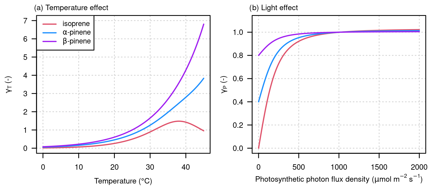
Figure 4 Dependence of activity factors on (a) temperature and (b) light variations for three BVOCs (equations from Guenther et al., 1995, 2012; T₂₄ and T₂₄₀ are fixed to 294 K in this figure).

Other activity factors could be added to represent the effect of leaf age and water stress. In this study, emissions are calculated per measure of leaf biomass, considering an average emission for all leaves in the canopy. In addition, we assume that in June and July, tree foliage is fully developed, and leaf area and dry biomass are constant. Therefore, no activity factor is added to modulate emissions according to the fraction of new, growing, mature, and old foliage (Guenther et al., 2012).

Several studies also introduce an activity factor to represent the impact of soil moisture and water stress on isoprene emissions (Guenther et al., 2012; Jiang et al., 2018; Bonn et al., 2019; Otu-Larbi et al., 2020; Wang et al., 2022). Although urban trees planted in reduced soil volumes may be subject to water stress (Lüttge and Buckeridge, 2023), the resolution of the CTM does not allow us to accurately simulate the soil water content in an urban environment, so no activity factor modulating isoprene emissions as a function of water content is taken into account here.

3.2 Integration of individual tree BVOC emissions in CHIMERE

After estimating the biogenic emissions of each tree in the city of Paris, these emissions are integrated into the CHIMERE CTM. To do this, they must be spatialized and speciated, as detailed in this section.

3.2.1 Integration of individual tree BVOC emissions on the CTM grid

First, each tree is located within the CTM grid using its precise position given in the Paris tree inventory and the coordinates of the CTM grid. The product of the dry biomass and the emission factor (DB_tEF_t,k) is then summed for all trees belonging to the same cell to compute the BVOC emission rates (ER${}_{i,j,k}$ in $\mathrm{\mu }\mathrm{g}{\mathrm{m}}^{-\mathrm{2}}{\mathrm{h}}^{-\mathrm{1}}$) as

$$\begin{array}{}\text{(2)}& {\text{ER}}_{i,j,k}={\displaystyle \frac{\mathrm{1}}{\mathrm{\Delta }{x}_{i,j}\mathrm{\Delta }{y}_{i,j}}}\sum _{t\in i,j}\left({\text{DB}}_{t}E{F}_{t,k}\right){\mathit{\gamma }}_{T_{i,j,k}}\cdot {\mathit{\gamma }}_{P_{i,j,k}},\end{array}$$

where Δx_i,j and Δy_i,j are the size of the cell (i,j) in the x and y directions (m), here both equal to 1000 m. A map of the dry biomass integrated on the CTM grid cells is shown in Fig. 5.

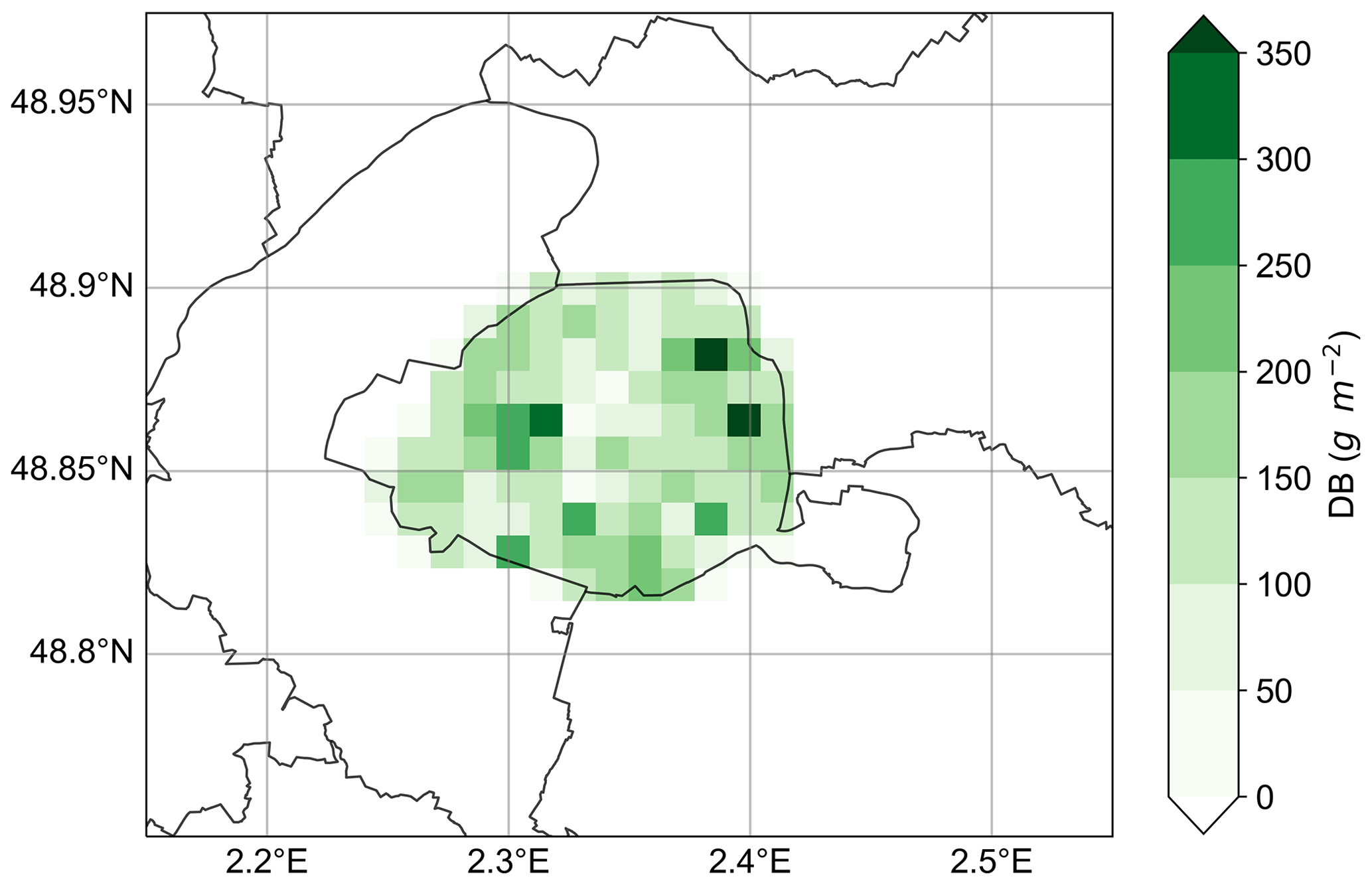
Figure 5 Tree leaf dry biomass computed over Paris from the Paris tree database and McPherson et al. (2016) with a spatial resolution of 1 km × 1 km.

The average cell dry biomass over Paris is 130 g m⁻² and can reach 390 g m⁻² in cells containing large parks or cemeteries. The Paris tree inventory does not include all the trees in the Vincennes and Boulogne woods; however, the emissions of these large woods are already modeled at the regional scale using the land use approach. Thus, they are not considered in the Paris tree inventory added in the simulation bioparis in order to avoid overlapping of emissions (Fig. 6). Note that except for Fig. 2, all the maps presented in this study represent the average value of the variable in the 1 km × 1 km grid cells without any post-processing.

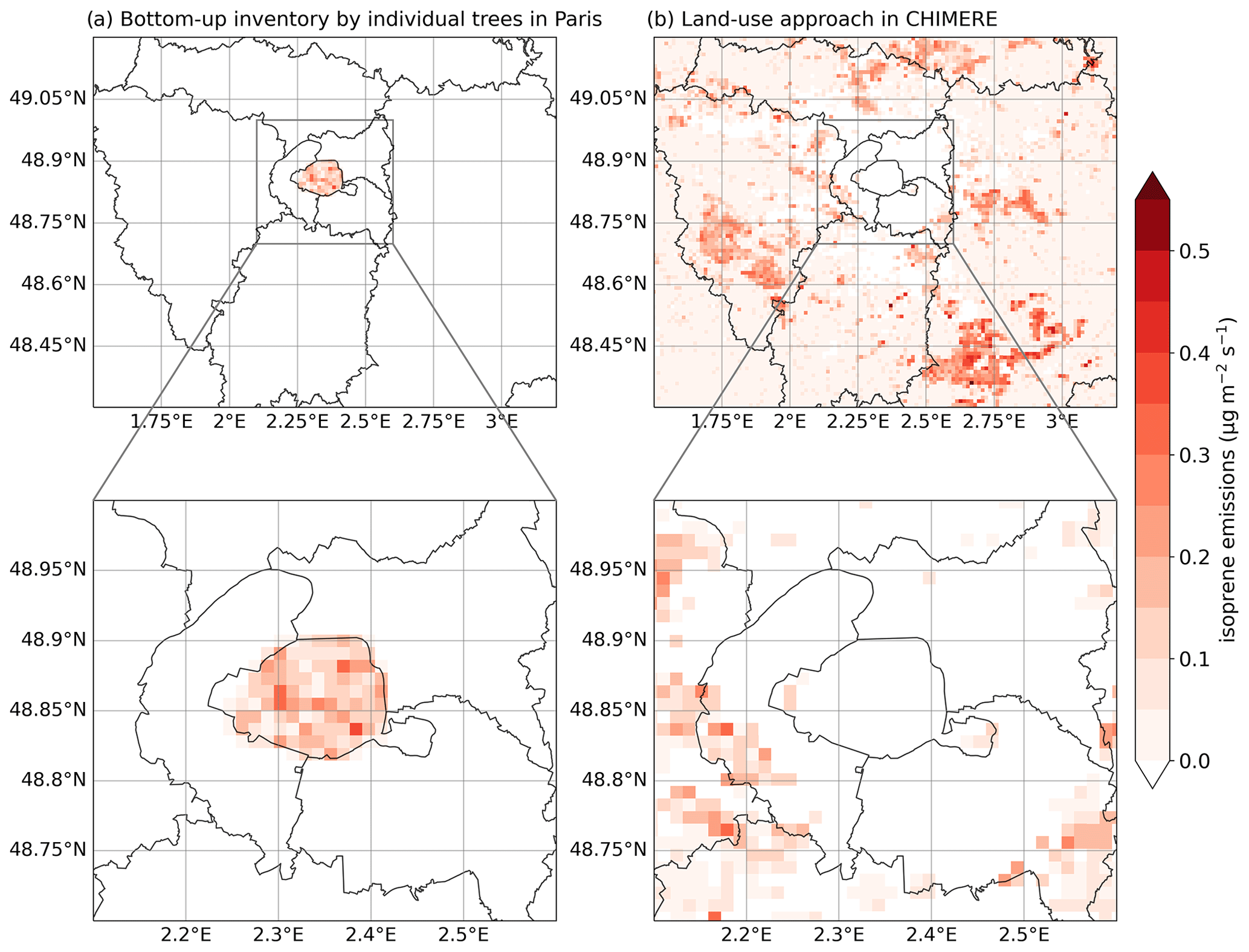
Figure 6 Comparison of the 2-month-averaged isoprene emissions with (a) the bottom-up inventory and (b) with the land cover approach in CHIMERE over Île-de-France and greater Paris.

3.2.2 Speciation and aggregation of BVOC species

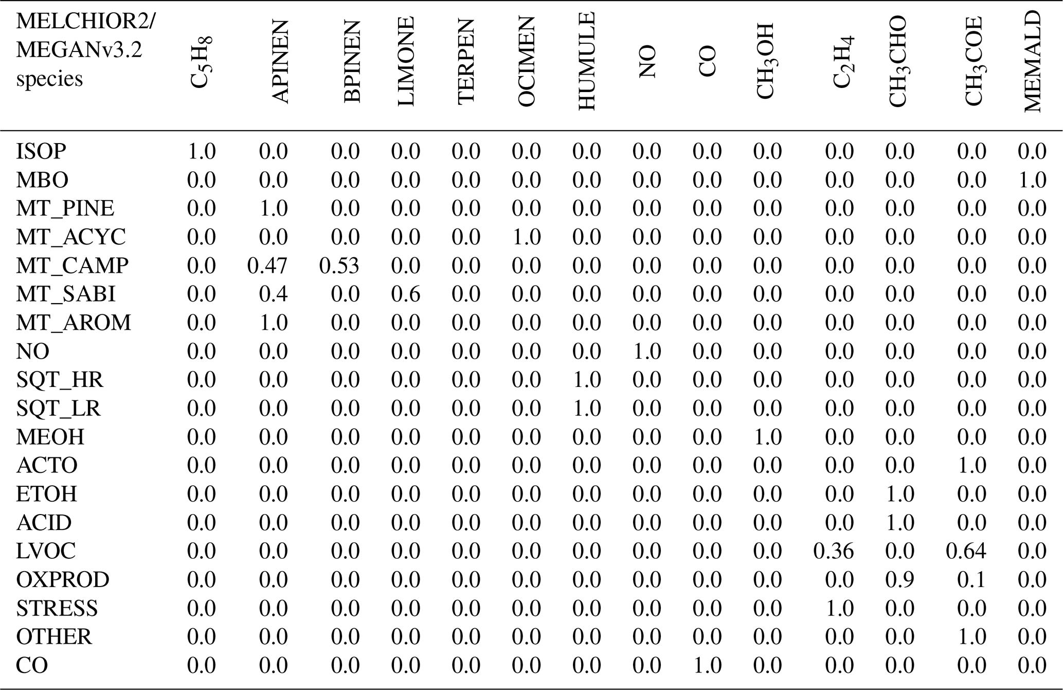
The emission factors of MEGANv3.2 are estimated for different categories of BVOCs, which are presented in the rows of Table D3. These BVOC categories need to be disaggregated into model species to be used in the CTM. The chemical scheme used in CHIMERE corresponds to MELCHIOR2, and the model species are shown in the columns of Table D3. To disaggregate the BVOC categories into model species, the BVOC categories are first speciated into detailed real species, which are then aggregated into the model species. The speciation in real BVOC species is done with a speciation matrix available in MEGANv3.2 code (downloaded at https://bai.ess.uci.edu/megan/data-and-code/megan32, last access: 10 July 2023). Then, the real BVOC species used in CHIMERE are speciated and aggregated into MELCHIOR2 species. The product of the two matrices gives the speciation/aggregation matrix, as described in Table D3. Note that no specific speciation is applied to sesquiterpenes, which are all included in the model species humulene (HUMULE). Monoterpenes are speciated as α-pinene (APINEN), β-pinene (BPINEN), limonene (LIMONE), and ocimene (OCIMEN); other VOCs (OVOCs) represent ethylene (C₂H₄) and oxygenated VOCs (CH₃OH, CH₃CHO, CH₃COE, and MEMALD).

Then, the BVOC emissions from urban trees in Paris are added to the regional-scale BVOC emissions to estimate the BVOC emissions over the Île-de-France region. Section 3.3 below details the complementarity between the bottom-up inventory for urban trees and the regional-scale PFT-based emissions.

3.3 Complementarity of the emissions computed by the bottom-up and the land use approaches

At the regional-scale, biogenic emissions are estimated using a land use approach with emission factors that depend on the land use and PFT, as described in Guenther et al. (2012). As the land use is urban over Paris, vegetation is not considered, and there are no biogenic emissions, as shown in Fig. 6a, which represents the 2-month-averaged isoprene emissions computed with the bottom-up inventory, and in Fig. 6b, which represents isoprene emissions computed with the land use approach in CHIMERE.

The bottom-up inventory allows accounting of local biogenic emissions in the city, but Fig. 6 shows that tree inventory and emissions are probably still missing in the Paris suburban area because there is currently no tree inventory for most of the urban areas outside Paris city. The order of magnitude of isoprene emissions computed by the bottom-up inventory seems coherent compared to regional-scale emissions. Emission rates in Paris (0.12 $\mathrm{\mu }\mathrm{g}{\mathrm{m}}^{-\mathrm{2}}{\mathrm{s}}^{-\mathrm{1}}$ on average for isoprene) are lower than those simulated over the large Île-de-France forests. This is also the case for other BVOC species, as shown in Appendix D5. The relative distribution of monoterpenes emitted is different between the urban and the regional scales, as shown in Fig. D3. In particular, there is relatively more β-pinene in the regional-scale emissions. This is due to the different vegetation species between the city and the regional scale and to the speciation of monoterpenes, which may be different.

The temporal variation in the spatially averaged emissions of different biogenic compounds is shown in Fig. 7. For all compounds, emissions are strongly correlated with temperature and sunlight. Over the 2-month periods, there are three emission peaks corresponding to periods of heatwaves with clear-sky conditions and air temperature reaching 35 °C. The impact of BVOC emissions on air quality is expected to be higher during these periods. Therefore, the effect of emissions on pollutant concentrations will be calculated both on the 2-month period and on the heatwave periods, which correspond to the following days: 15 to 18 June, 11 to 14 July, and 17 to 19 July. In terms of emitted compounds, isoprene is the most emitted biogenic species, followed by OVOCs. Monoterpenes and CO are emitted to a lesser extent, followed by sesquiterpenes and NO. This distribution of emissions is fairly typical of emissions calculated using the MEGAN model (Guenther et al., 2012; Ciccioli et al., 2023). In terms of emission intensity, some recent studies computing the BVOC emissions over Europe with plant-emission-specific models instead of using the PFT approach of MEGAN have reported that isoprene emissions may be overestimated by a factor of 3 in MEGANv2.1, while monoterpene and sesquiterpene emissions may be underestimated by a factor of 3, especially in summer (Jiang et al., 2019; Ciccioli et al., 2023). These discrepancies were attributed to the different vegetation classifications and emission factors at standard conditions. Using plant-emission-specific models, Jiang et al. (2019) found a better comparison to observations for isoprene and organic aerosol concentrations at the European scale, while around the Paris basin in summer, differences in emissions mainly concern monoterpenes and sesquiterpenes. In order to take these emission uncertainties into account in our study, sensitivity simulations are carried out by multiplying monoterpene and sesquiterpene emissions by a factor of 2 or 3.

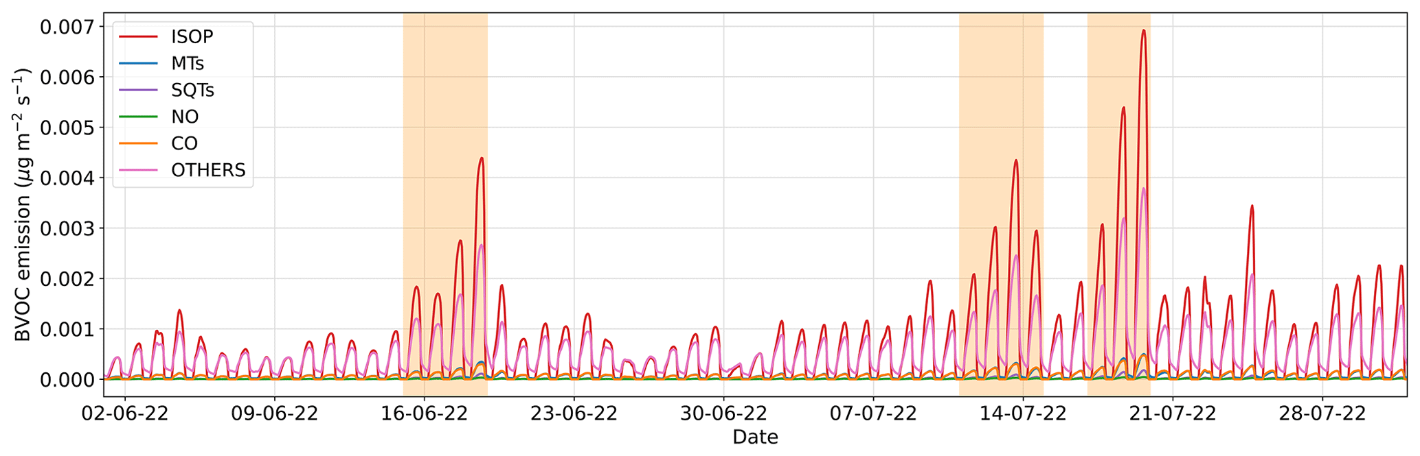
Figure 7 Temporal variation in the spatially averaged biogenic emissions computed over Paris with the bottom-up inventory. Heatwave periods are indicated by shaded orange areas.

4 Quantification of the impact of BVOC emissions from urban trees on air quality at the regional scale

Before studying the impacts of the bottom-up inventory, comparisons of simulated and observed key variables are performed to evaluate the simulation performance. Meteorological variables are first analyzed in Sect. 4.1.1, as biogenic emissions are strongly related to them. Then, Sect. 4.1.2 presents comparisons of modeled and observed pollutant concentrations at different air quality stations in Île-de-France. Simulations are performed with the emission factors presented above (REF) and with monoterpene and sesquiterpene emissions multiplied by a factor of 2 (REF-TX2) and 3 (REF-TX3).

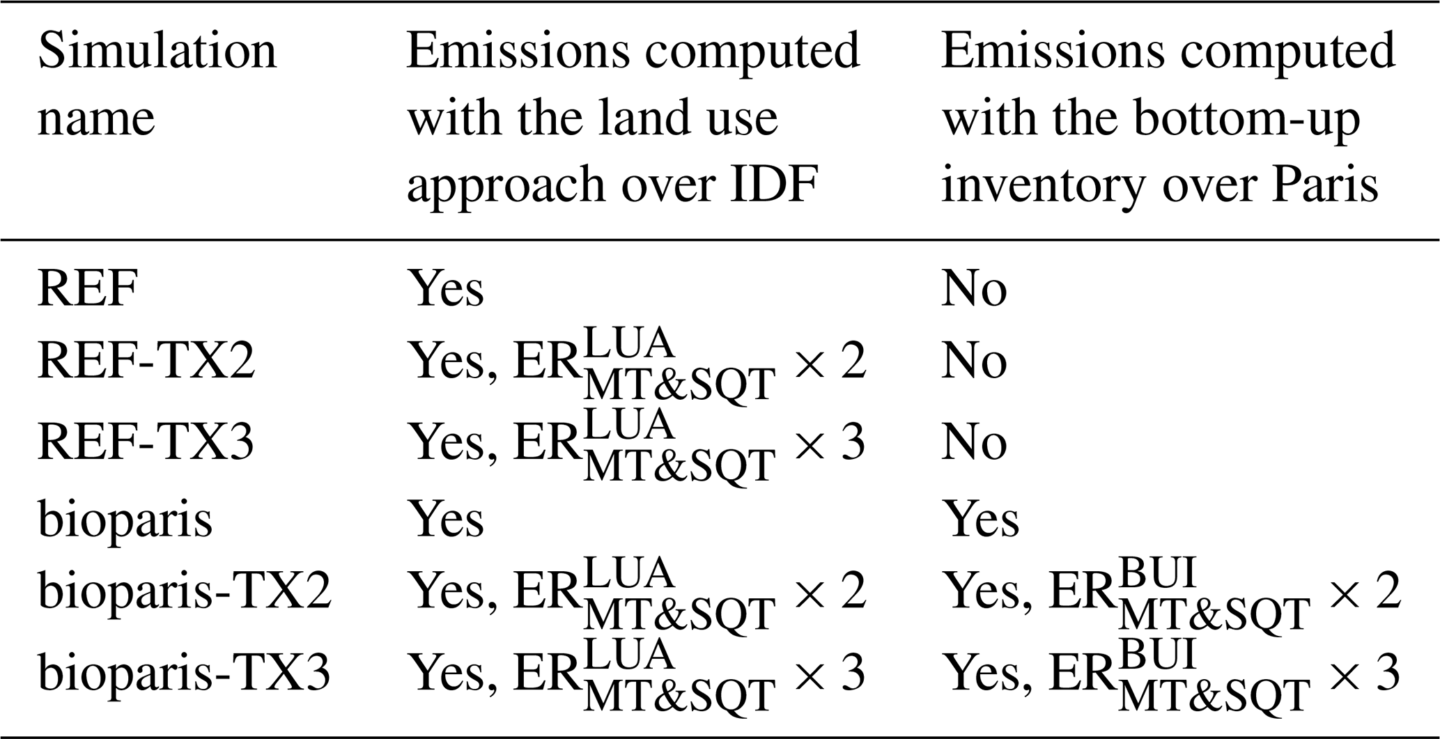
Then, to quantify the impacts of urban trees on air quality, simulations with the biogenic emissions from urban trees are performed and compared to the simulations without trees in Sect. 4.2. Three simulations with urban trees are performed, with one for each monoterpene and sesquiterpene emission scenario, which are referred to as bioparis, bioparis-TX2, and bioparis-TX3. All the simulations performed and the corresponding emissions are presented in Table 3.

Table 3 Simulation list with corresponding emission scenarios. ER stands for emission rate, SQT is for sesquiterpene, MT is for monoterpene, LUA is for land use approach, and BUI is for bottom-up inventory.

4.1 Validation of the reference simulations

4.1.1 Meteorology

The surface meteorological fields simulated by WRF-CHIMERE are compared to measurements performed at SIRTA (with 10 min time steps) in Fig. E1 and Table E1 and at seven weather stations operated by Météo-France (MF) (with hourly time steps) in Table E2. The comparison shows that the model simulates the 2 m air temperature with slight bias of +0.8 to 0.9 °C and the global shortwave radiation with a bias around +50 W m⁻² well. The other variables are also rather well simulated, with a slight overestimation of the relative humidity (bias of −6.3 at SIRTA and −9.4 % at MF stations) and of the surface atmospheric pressure (bias of +2.7 at SIRTA and +1.0 hPa at MF stations). The wind speed is overestimated (bias of +1.9 at SIRTA and +1.2 m s⁻¹ at MF stations) mainly because of the difference in representativeness between the average wind speed simulated in the first 24 m high vertical mesh and the wind measured at 10 m. A detailed description of the validation is provided in Appendix E.

4.1.2 Model–data comparisons of gas and particle concentrations

NO₂, O₃, OM, PM_2.5, isoprene, and monoterpene concentrations simulated by CHIMERE for the three emission scenarios REF, REF-TX2, and REF-TX3 are compared to observations performed at different measurement stations over Île-de-France in Appendix F. As shown in Table F1, NO₂ and O₃ concentrations compare well to observations (the most strict performance criteria defined by Hanna and Chang, 2012, are respected for all statistical indicators), and the impact of emission scenarios is low. PM_2.5 and OM concentrations are more sensitive to the emission scenarios, and the comparisons to observations are better at suburban and urban stations with the REF-TX3 scenario. Nevertheless, the less strict performance criteria by Hanna and Chang (2012) are respected for all statistical indicators in REF-TX2 and REF-TX3 simulations. The simulations tend to underestimate isoprene and monoterpene concentrations compared to observations. This could be partly explained by the absence of biogenic emissions inside Paris in the reference simulations. A more detailed description of comparisons between simulations and observations is given in Appendix F.

4.2 Impact of biogenic emissions from urban trees on isoprene, monoterpene, ozone, organic matter, and PM_2.5 concentrations

4.2.1 Impact of urban tree biogenic emissions on isoprene and monoterpene concentrations

Comparisons of the hourly concentrations of isoprene and monoterpenes observed and simulated in the reference case (REF-TX2) and with the urban tree biogenic emissions (bioparis-TX2) at PRG presented in Fig. 8.

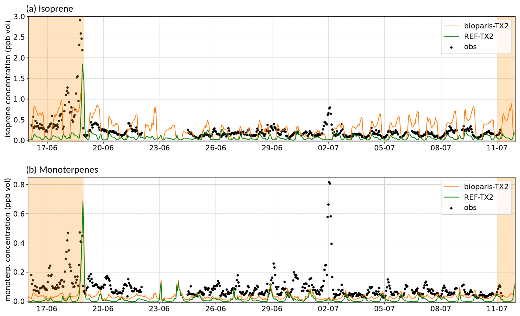
Figure 8 Observed and simulated hourly concentrations of (a) isoprene and (b) monoterpenes at the PRG station with (bioparis-TX2) and without (REF-TX2) the bottom-up biogenic emission inventory. Heatwave periods are indicated by shaded orange areas.

Figure 8a shows that isoprene concentrations simulated at PRG are underestimated in the reference simulation compared to the measurements. The inclusion of the urban tree biogenic emissions allows a better representation of the isoprene concentrations (decrease in the normalized absolute difference (NAD) from 0.57 (REF-TX2) to 0.38 (bioparis-TX2) and increase in the correlation from 0.38 (REF-TX2) to 0.42 (bioparis-TX2)). However, in the bioparis-TX2 simulation, the daytime concentrations are overestimated on 16, 17, 19, and 20 June and between 2 and 10 July by about a factor of 1.5, but the concentration peak around 18 June is underestimated. At night, non-zero isoprene concentrations are measured, and the simulated concentrations are almost zero because isoprene is emitted only during the day by biogenic emissions and has a short lifetime (τ_OH≈ 1.5 h with [OH] =10⁶ molec. cm⁻³, Atkinson and Arey, 2003b). Isoprene is also emitted by road traffic, according the VOC speciation used (Theloke and Friedrich, 2007; Baudic et al., 2016), but in the model, traffic emissions are too low at night to represent the measured concentrations. This model–measurement discrepancy could be due to a measurement artifact or to missing anthropogenic sources of isoprene at night. In view of the uncertainties in the measurements, the model provides a satisfactory representation of the order of magnitude of isoprene concentrations.

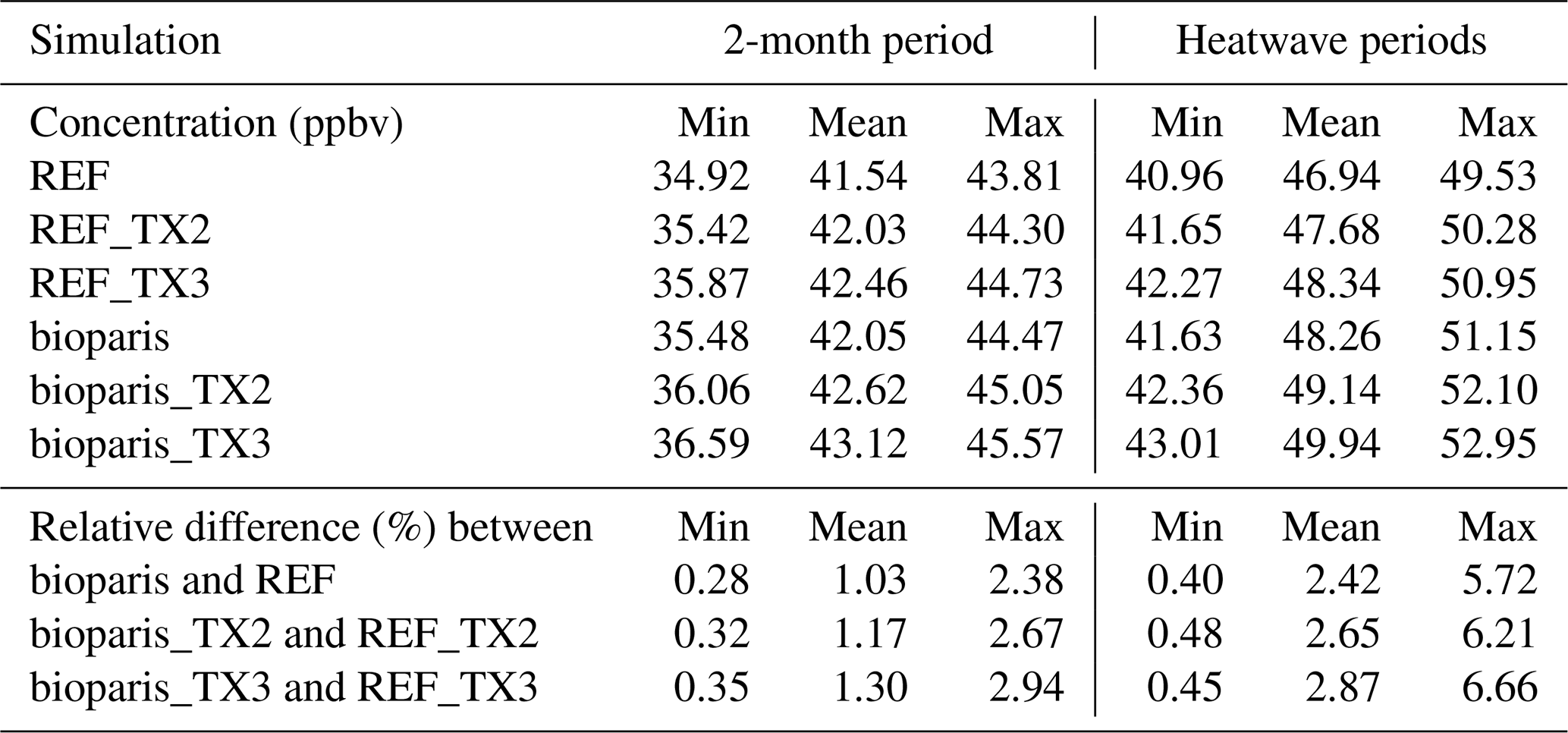
Table 4 presents the averaged isoprene and monoterpene concentrations and the relative impact of bioparis during the 2-month period and heatwaves. Note that the relative difference in the concentrations is calculated on an hourly time step and then averaged over the 2-month or heatwave periods. The min and max columns in the tables correspond to the minimum and maximum values of the time-averaged concentration or relative difference. As seen previously, biogenic emissions are driven by environmental variables, in particular temperature and solar radiation. To determine whether the effect of local biogenic emissions is greater during heatwaves, isoprene concentrations are also compared during these periods. It is especially relevant to quantify this effect because the frequency of these episodes is expected to increase in the future due to climate change (IPCC, 2021). The heatwave period refers to the averaged concentrations on the following days: 15, 16, 17, and 18 June and 11, 12, 13, 14, 17, 18, and 19 July. During these periods, high air temperatures and clear-sky conditions were observed as shown in Fig. E1. Table 4 shows that at the scale of the city of Paris, local isoprene emissions significantly increase isoprene concentrations (+1100 % on average). The effect of bioparis during the heatwave periods is higher (+2400 % on average) because emissions during that period are higher. As the TX2 and TX3 scenarios do not modify isoprene emissions, there is no impact on isoprene concentrations.

Table 4 Comparison of minimum, mean, and maximum isoprene and monoterpene concentrations averaged in Paris for each simulation and relative difference between the bioparis and the reference simulations during the 2-month and heatwave periods.

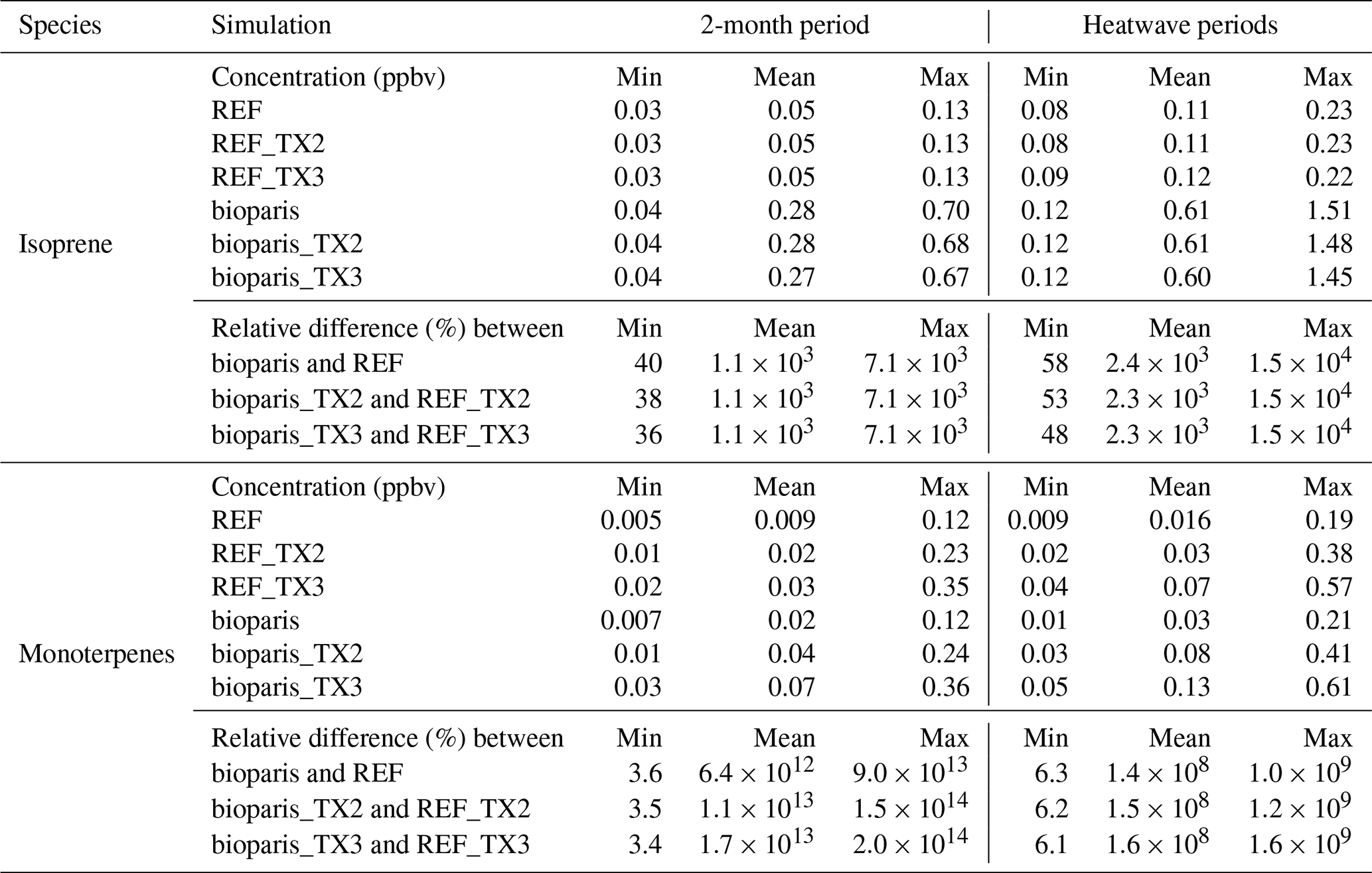
The comparison of monoterpene concentrations presented in Fig. 8b shows that monoterpenes are underestimated at PRG in the reference simulation, and the addition of the urban tree emissions strongly increases the monoterpene concentrations. However, the simulated concentrations still underestimate the observations, even with the bioparis-TX2 scenario, probably because of missing anthropogenic sources (Jo et al., 2023). Like isoprene, Table 4 shows that the addition of monoterpene emissions greatly increases the monoterpene concentrations by 6.4×10¹² % on average over the 2-month period and by 1.4×10⁸ % during the heatwave periods. Monoterpene concentrations logically increase when their emissions are multiplied by 2 (TX2) or 3 (TX3), but the simulated concentrations underestimate the measurements. This discrepancy raises the question of potentially missing local sources of vegetation that emit monoterpenes in the area of measurement.

4.2.2 Impact of urban tree biogenic emissions on organic matter and particles concentrations

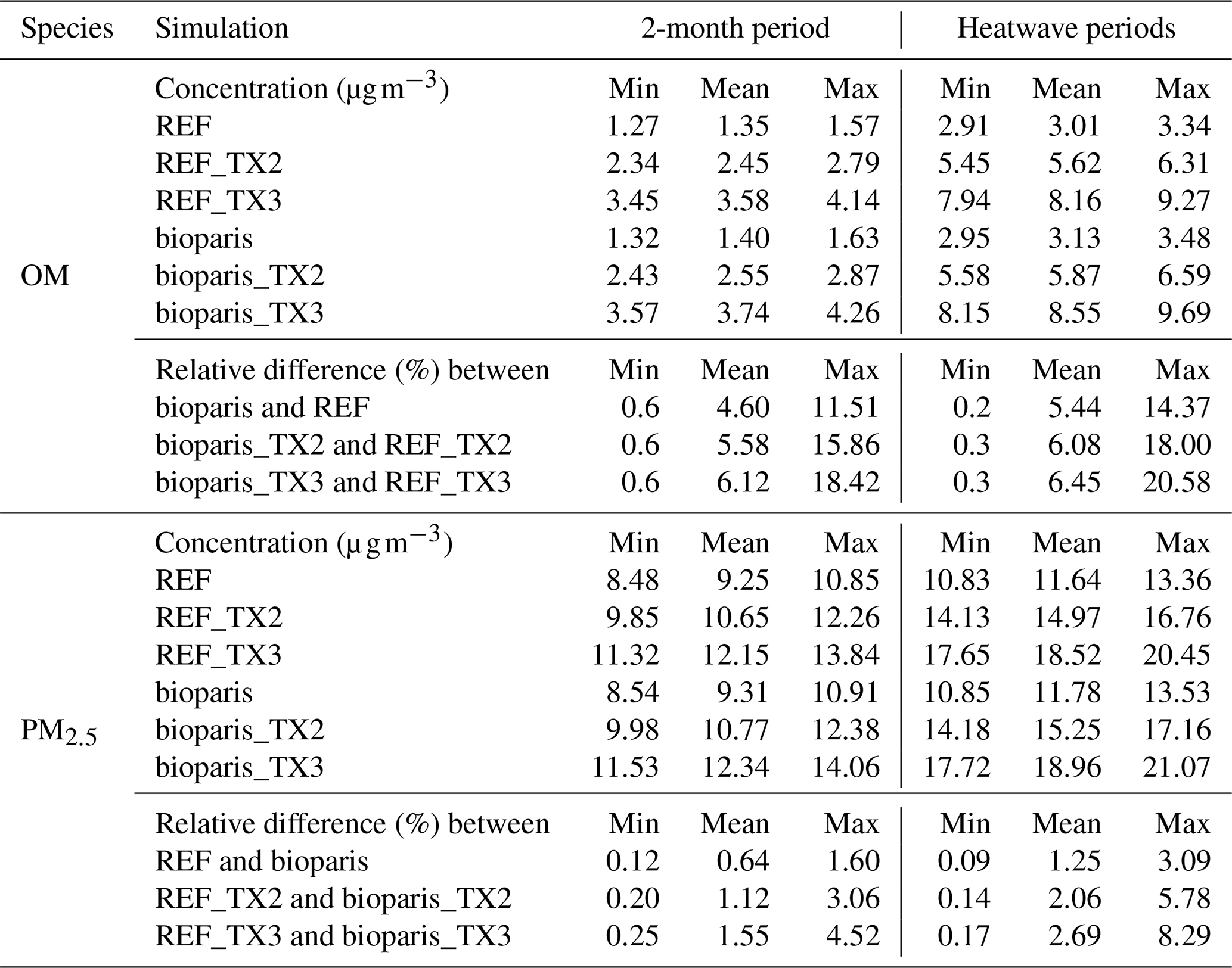
Figure 9 compares the observed and simulated OM concentrations at the (Fig. 9a) PRG and (Fig. 9b) Halles stations. It shows that the impact of the urban biogenic emissions on the PRG site is smaller for OM concentrations than for isoprene and monoterpene concentrations. The increase in OM concentrations with urban tree biogenic emissions in the Halles site is mainly visible during the heatwaves (Fig. 9b). The urban biogenic emissions lead to an increase in OM concentrations on average over Paris of 4.6 % during the 2-month period, as shown in Table 5. The increase in the OM concentrations is slightly larger when terpene emissions are doubled (+5.6 %) and tripled (+6.1 %). Due to larger biogenic emissions, the increase in OM concentrations is also larger during the heatwave (+5.4 %).

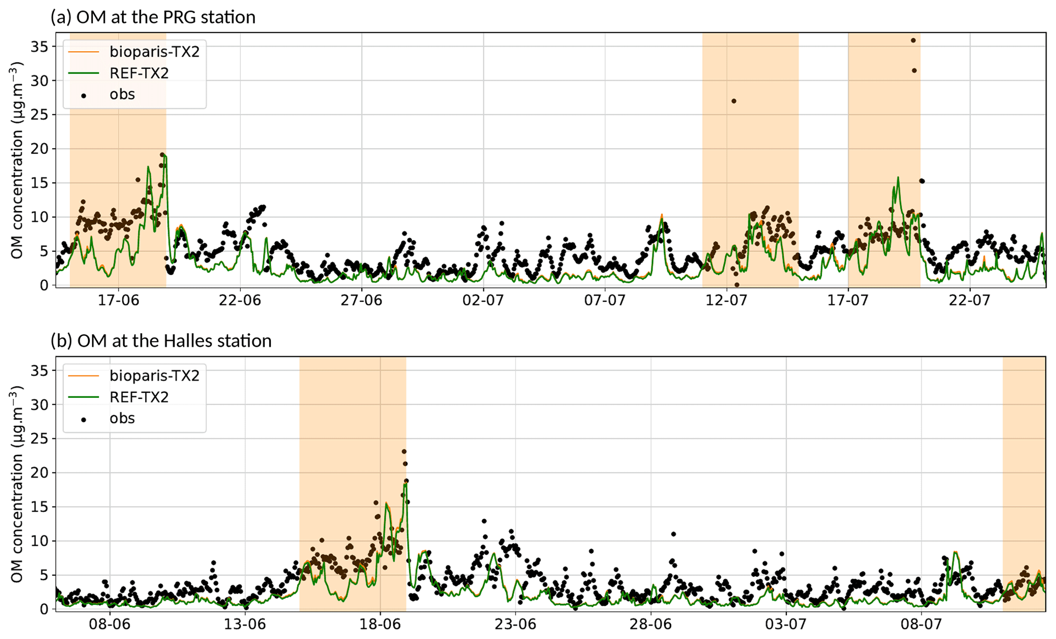
Figure 9 Observed and simulated hourly concentrations of organic matter (OM) at the (a) PRG and (b) Halles stations with (bioparis-TX2) and without (REF-TX2) the urban biogenic emission inventory. Heatwave periods are indicated by shaded orange areas.

Table 5 Comparison of minimum, mean, and maximum organic matter (OM) and PM_2.5 concentrations averaged in Paris for each simulation and relative difference between the bioparis and the reference simulations during the 2-month and heatwave periods.

The impact of the urban biogenic emissions is also less visible on hourly concentrations of PM_2.5, so the relative differences in OM and PM_2.5 concentrations are mapped in Figs. 10 and 11. The two top panels present the REF-TX2 concentrations and the relative difference between bioparis-TX2 and REF-TX2 concentrations averaged for the 2-month period. The same maps are presented in the two lower panels but with the concentrations averaged for the heatwave periods.

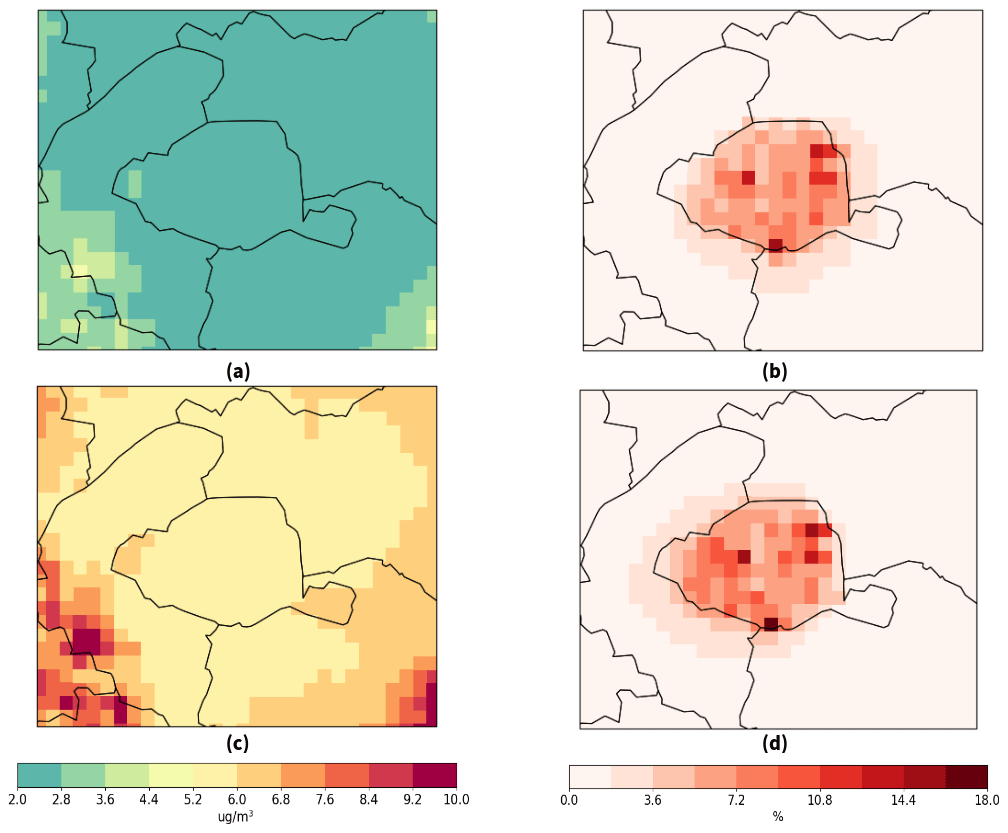
Figure 10 Average OM concentrations (µg m⁻³) simulated by CHIMERE (REF-TX2) during (a) the whole period and (c) the heatwave, and the relative difference in the OM concentrations with the urban tree biogenic emissions (bioparis-TX2) during (b) the whole period and (d) the heatwave.

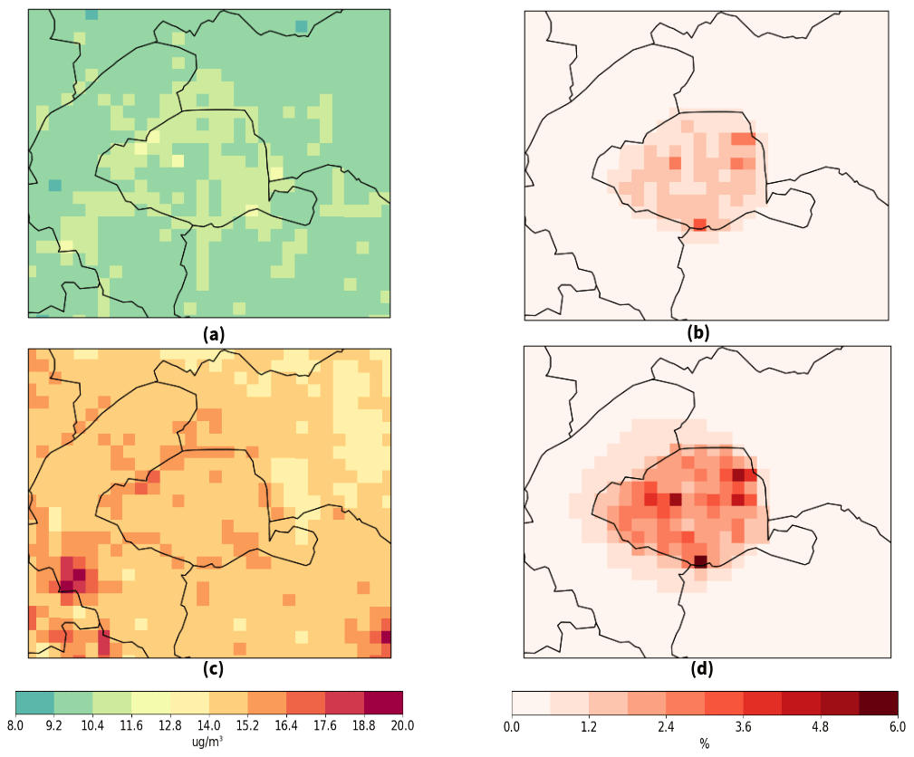
Figure 11 Average PM_2.5 concentrations (µg m⁻³) simulated by CHIMERE (REF-TX2) during (a) the whole period and (c) the heatwave, and the relative difference in the PM_2.5 concentrations with the urban tree biogenic emissions (bioparis-TX2) during (b) the whole period and (d) the heatwave.

Figure 10 shows the spatial variability in the local biogenic emission effect and that the increase in OM concentrations is due to emissions from urban trees remaining localized over Paris. It is greater in cells with a large tree biomass (Fig. 5), where biogenic emissions are also larger, in particular monoterpenes (Fig. D2) and sesquiterpenes (Fig. D4). This correlation shows that biogenic emissions from urban trees contribute strongly to local OM formation. The increase in OM concentrations is slightly larger during the heatwave periods, as shown in Table 5. The impact of urban emissions extends a little further during these periods.

The increase in PM_2.5 concentrations is lower than for OM, but the spatial distribution is similar. The impact remains localized over Paris (+0.6 % on average) and is strongest during heatwaves (+1.3 %), as shown by the maps in Fig. 11 and Table 5. The increase in PM_2.5 is larger when monoterpene and sesquiterpene emissions are doubled (TX2) and tripled (TX3) (Table 5). This underlines the importance of terpenes in the formation of particulate matter.

4.2.3 Impact on ozone concentrations

Ozone concentrations also increase with the urban tree biogenic emissions (+1 % on average), especially during the heatwave periods (+2.4 %). The increase in O₃ concentrations is also mostly localized in the Paris city and extends to the Paris suburbs during heatwaves (Fig. 12). Table 6 shows that doubled or tripled monoterpene and sesquiterpene emissions increase ozone concentrations, but the increase is relatively lower than for OM and PM_2.5. This suggests that ozone formation is less sensitive to monoterpene and sesquiterpene emissions, which mostly impact the formation of organic matter.

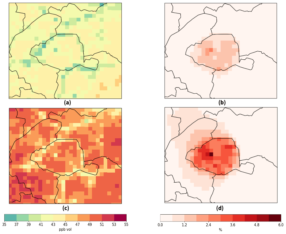
Figure 12 Average O₃ concentrations (ppbv, parts per billion by volume) simulated by CHIMERE (REF-TX2) during (a) the whole period and (c) the heatwave, and the relative difference in the O₃ concentrations with the urban tree biogenic emissions (bioparis-TX2) during (b) the whole period and (d) the heatwave.

Table 6 Comparison of minimum, mean, and maximum ozone concentrations averaged in Paris for each simulation and relative difference between the bioparis and the reference simulations during the 2-month and heatwave periods.

The urban biogenic emissions mainly increase O₃ concentrations during the day, as the concentrations of biogenic species are higher, and O₃ is formed during daytime influenced by solar radiation and temperature. The impact of the biogenic bottom-up inventory on maximal daily ozone concentrations (8 h moving average) is also evaluated, as this value is used in the French air quality standards (LCSQA, 2016). The bottom-up inventory increases the ozone maximal 8 h concentrations on average over the 2 months by around 0.6 % and by 1.2 % during heatwaves in all scenarios. The maximal impact goes from 4.0 % to 4.8 %, according to the biogenic emission factor scenario, on average over the 2-month period and from 7.6 % to 8.5 % during heatwaves.

5 Conclusions

This study presents the development of an inventory of biogenic emissions from urban trees using a bottom-up approach and based on the city tree inventory, tree allometric relations and empirical emission equations. The emissions are computed for individual urban trees and integrated into CHIMERE-WRF simulations to quantify the impact of urban trees on pollutant concentrations.

Air quality simulations over the Paris region during the 2 months of June and July 2022 lead to simulated NO₂, O₃, and PM_2.5 concentrations that are globally consistent with measurements. OM, isoprene, and monoterpene concentrations are underestimated, but they increase when emissions from urban trees are taken into account. Over Paris city, urban trees induce a significant increase in OM concentrations of 4.6 % on average over the 2 months and of 5.4 % during the heatwave periods. This increase can reach 11.5 % locally on average over the 2 months and 14.4 % during the heatwave period. The increase in OM concentrations is sensitive to monoterpene and sesquiterpene emissions and remains localized over Paris city where the urban trees are located. O₃ concentrations also slightly increase due to the urban tree emissions by 1.0 % on average over the 2 months and by 2.4 % during the heatwaves. This increase can locally reach 2.4 % on average over the 2 months and 5.7 % during the heatwaves. The increase in O₃ concentrations during the heatwave periods extends to the Paris suburbs, which is further than for OM. These values correspond to temporal averages, but the effect of urban emissions on OM, PM_2.5, and O₃ is higher during the daytime when biogenic emissions and photolysis occur, aggravating O₃ peaks during heatwaves. This shows that urban tree emissions have a large impact on air quality, and low-emitting tree species should be favored in cities. In particular, we recommend choosing to plant tree species that emit few terpenes.

OM concentrations are particularly sensitive to terpene emissions. It is essential to better estimate terpene emission factors of urban and suburban trees. Furthermore, it should be noted that part of the urban vegetation (in private areas) and part of the suburban vegetation were not taken into account in this study, as the tree inventory is only available for the public trees of Paris city. The effect of urban and suburban trees on air quality is therefore probably underestimated, and this may contribute to the underestimation of monoterpene and OM concentrations observed. Tree inventories should be set up systematically in more cities and their suburbs. This could be completed with methods for characterizing urban vegetation using aerial images, for example. This methodology for building a BVOC bottom-up inventory could be easily applied to other cities that have a tree inventory.

Further work would involve improving the estimation of the tree-scale biogenic emissions by improving the spatial resolution of the meteorological fields. Speciation of monoterpenes and oxygenated VOCs emitted into model chemical species is assumed to be identical for each tree species. A speciation of monoterpenes according to the tree species, as done in Steinbrecher et al. (2009), could be introduced. However, as this speciation does not include all the tree species found in Paris, the speciation should be enriched with other data. Finally, urbanization may induce very local modifications of climate in streets, with potentially higher temperatures, modified solar radiation due to building shading, and water stress if trees are planted in limited soil volume. These processes are not taken into account in this study, where the spatial resolution is typical of regional urban studies, i.e., 1 km × 1 km.

Appendix A: Detailed description of the experimental measurements

A1 Measurements performed at SIRTA

Isoprene was measured with a gas chromatograph equipped with a flame ionization detector (GC-FID), airmoVOC C2–C6 (Chromatotec, Saint-Antoine, France). The instrument is described in detail in Gros et al. (2011). Calibration was performed using a NPL (National Physical Laboratory, Teddington, UK) standard. Uncertainty is estimated to be less than 15 %. Monoterpenes were measured at SIRTA using a proton transfer reaction quadrupole mass spectrometer (PTR-Q-MS) from Ionicon Analytik (Innsbruck, Austria) with a time resolution of 5 min. This instrument was implemented at SIRTA for long-term measurements in early 2020, and its operating conditions are described in Simon et al. (2023). The ambient air was sampled at 15 m, 1 h blank measurements were performed every 13 h, and calibrations were done every month with a NPL standard containing α-pinene. Monoterpenes were measured at the mass-to-charge ratio ($m/z$) 137, and the associated uncertainties for the period of June–July 2022 were 32 %, while the mean detection limit was of 25 ppt (parts per trillion).

A2 Measurements performed at PRG

Gas and aerosol sampling at the PRG site are performed at 30 m a.g.l. VOCs were measured at the PRG site using a proton transfer reaction time-of-flight mass spectrometer (PTR-ToF-MS; PTR 4000 X2, Ionicon Analytik, Austria) equipped with a CHARON inlet, which is already extensively described elsewhere (Jordan et al., 2009; Eichler et al., 2015; Müller et al., 2017; Leglise et al., 2019). The instrument has been programmed to automatically switch between gas and particle phases and was working at 2.6 mbar and at $E/N=$ 120 Td. Gas was sampled at the top of a seventh floor building through a 12 m long Teflon tubing with a 17.5 mm inner diameter. The flow in this main line was fixed at 40 L min⁻¹ until a glass manifold where all gas-phase instruments sampled ambient air. Sensitivity and background have been regularly controlled during the course of the experiment using a pure nitrogen cylinder (99.99999 % purity; Linde) and a certified gas standard (containing 10 VOCs at 100 ppb; NPL), thus providing quantitative measurement with an uncertainty typically of the order of 10 ppt.

Table A1 List of Airparif stations with the species measured and used in this study.

A3 Measurements performed at the Halles

In the Halles station, NO₂ concentrations are measured by chemiluminescence detection with an AC32M analyzer from ENVEA (formerly Environnement SA) with a measurement uncertainty of 10 %. O₃ concentrations are measured by ultraviolet (UV) photometry with an O342e analyzer from ENVEA with a measurement uncertainty of 11 %. PM_2.5 is measured with a Fidas 200 analyzer from Palas and certified technically compliant by the Laboratoire Central de la Surveillance de la Qualité de l'Air (LCSQA) for continuous, real-time regulatory monitoring of PM₁₀ and PM_2.5 fractions based on the optical detection of light scattered by aerosols (Lorenz–Mie solution). The uncertainties associated with the measurement are estimated to 9 %. More information on the certified devices for regulatory air quality measurement is available (in French) at https://www.lcsqa.org/system/files/media/documents/Liste%20appareils%20conforme%20mesure%20_qualit%C3%A9%20air%20M%C3%A0J_13-05-20_v2_0.pdf (last access: 5 May 2024).

Appendix B: Characteristics of trees in the Paris tree database

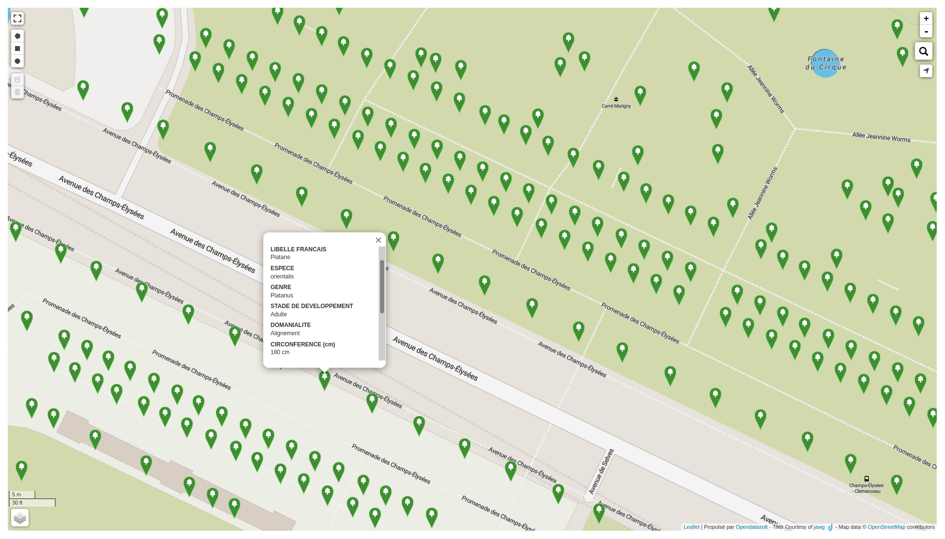
Figure B1 Screenshot of the Paris tree database near Avenue des Champs-Élysées (Municipality of Paris, 2023).

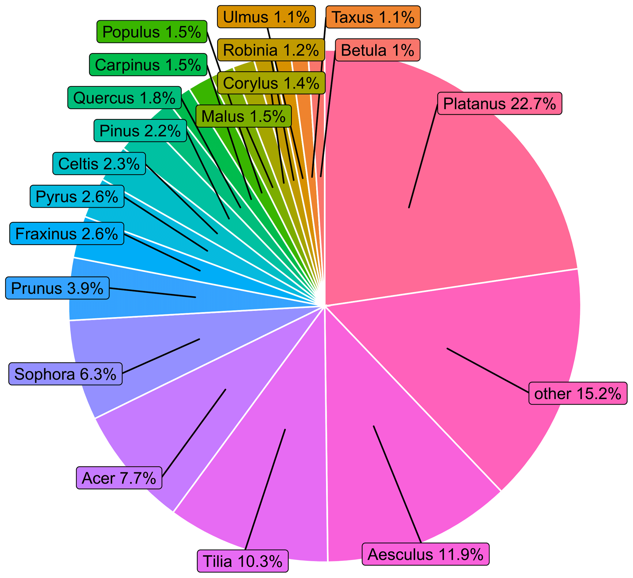
Figure B2 Proportion (%) of each tree genus in Paris (only genera with P> 1 % are shown; the rest of the trees are in the “other” category).

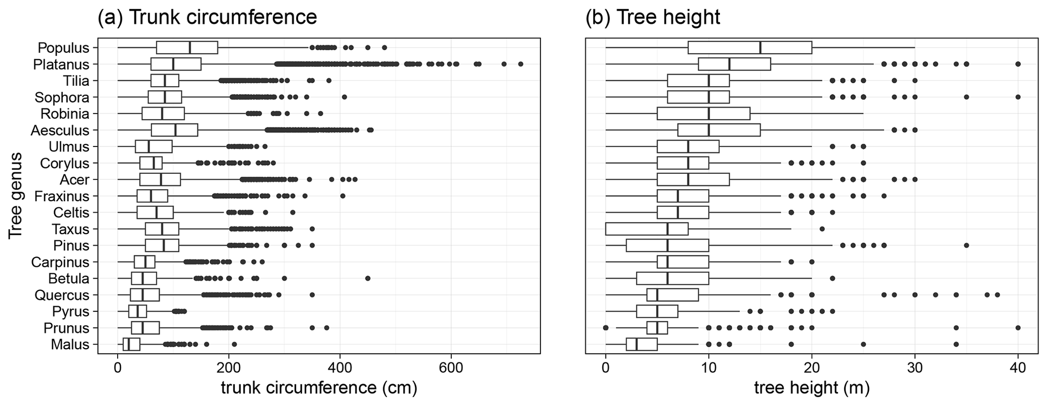
Figure B3 Box plot of the (a) trunk circumference and (b) tree height of the most dominant tree genera.

Appendix C: Average air temperature simulated by WRF

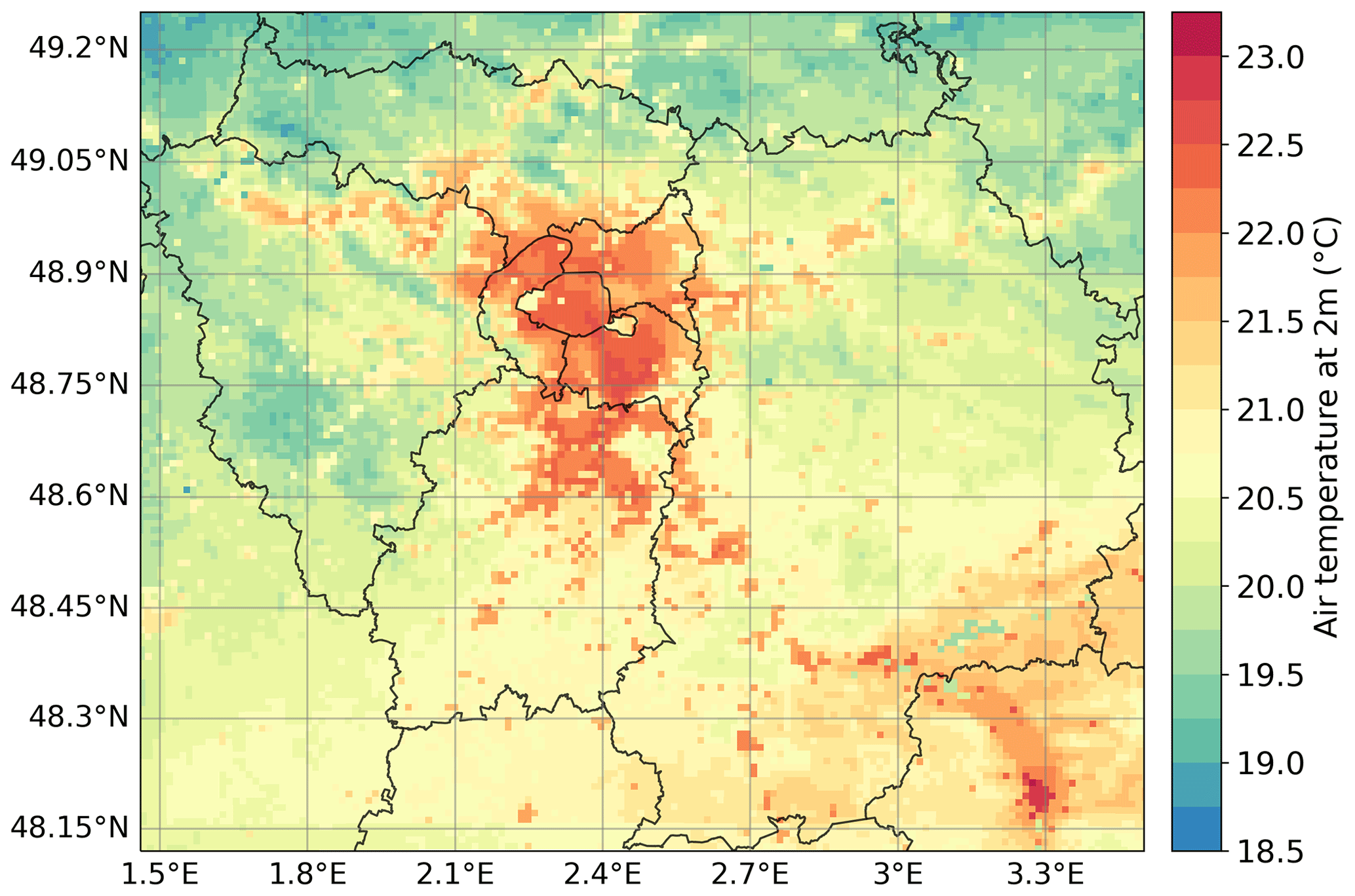
Figure C1 The 2-month-averaged air temperature at 2 m simulated by WRF in the IDF1 domain.

Appendix D: BVOC emissions

D1 Estimation of the tree dry biomass

Table D1 US reference cities and climates used in the McPherson et al. (2016) study ranked from the closest to the farthest from the Parisian climate. The last column refers to Köppen climate classification (Paris region is Cfb).

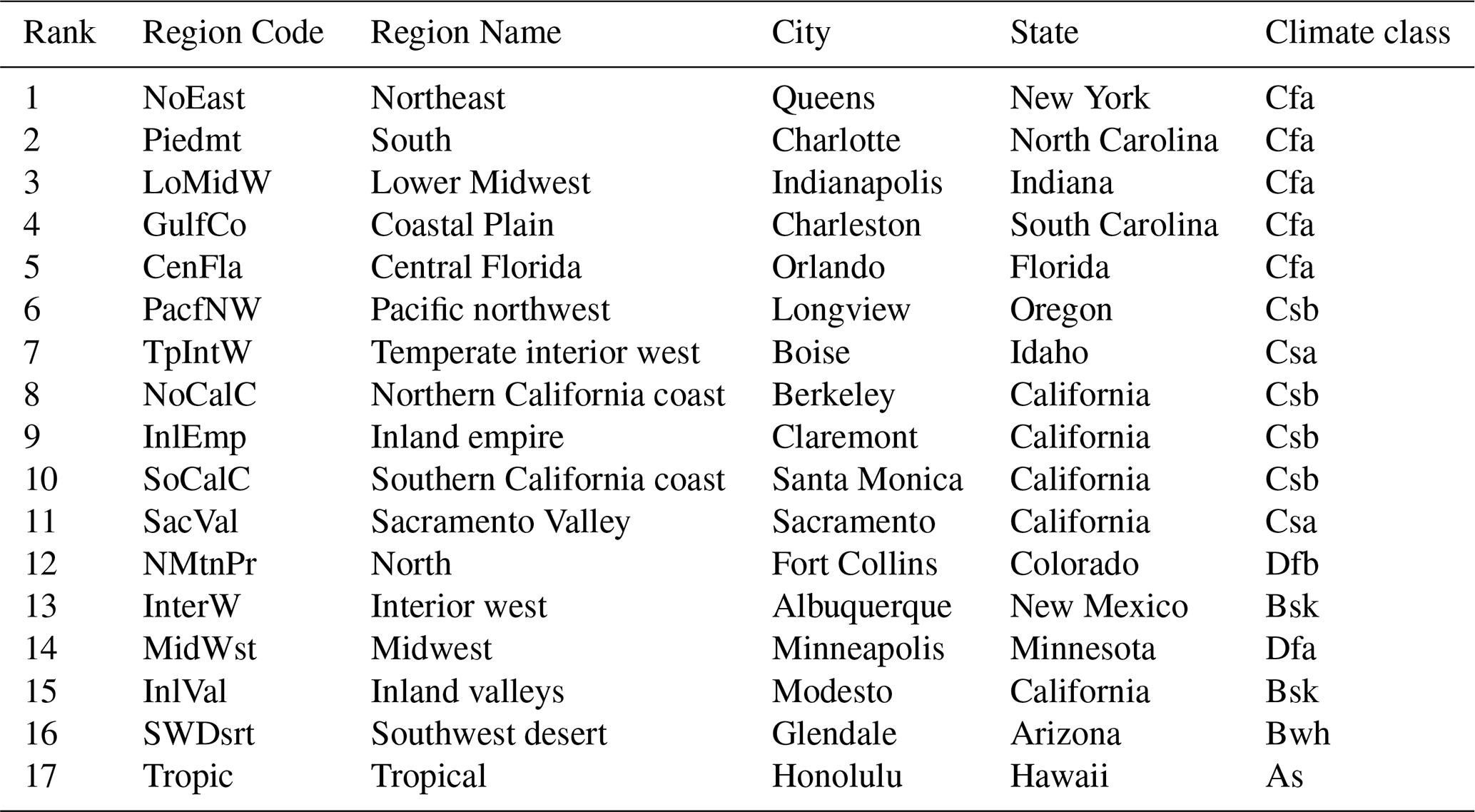
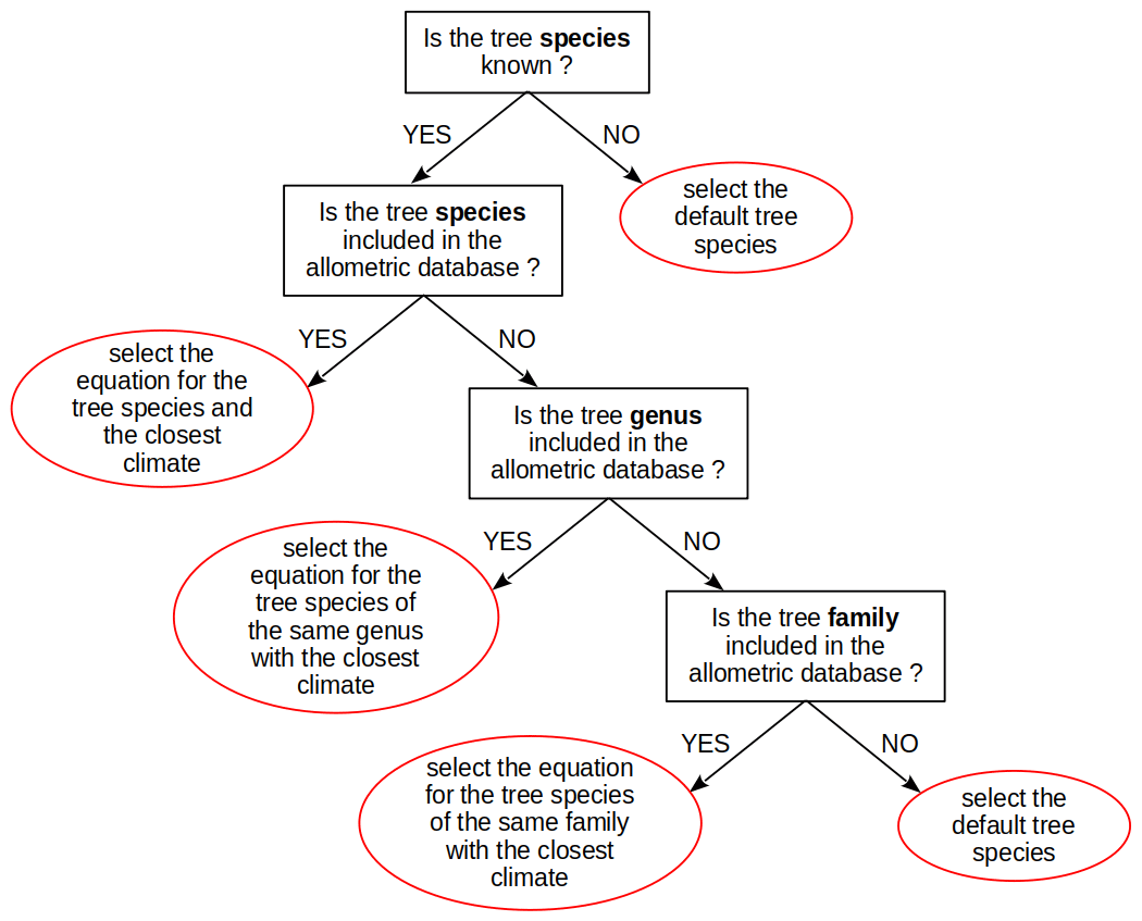
Figure D1 Decision tree to select the tree category to be used for each Paris tree. The tree category and corresponding allometric database refers to McPherson et al. (2016).

For Planatus × hispanica (London plane),

$$\begin{array}{}\text{(D1)}& \text{LA}=\exp \left[a+b\ln \left(\ln \left(\text{DBH}+\mathrm{1}\right)\right)+{\displaystyle \frac{\text{MSE}}{\mathrm{2}}}\right],\end{array}$$

with $a=-\mathrm{2.06877}$, b=5.77886, and MSE (mean squared error) =0.27978.

For Acer platanoides (Norway maple),

$$\begin{array}{}\text{(D2)}& \mathrm{\text{LA}}=\exp \left[a+b\ln \left(\ln \left(\text{DBH}+\mathrm{1}\right)\right)+\left(\sqrt{\text{DBH}}\times {\displaystyle \frac{\text{MSE}}{\mathrm{2}}}\right)\right],\end{array}$$

with $a=-\mathrm{0.55184}$, b=4.27852, and MSE =0.07518.

For Prunus serrulata (Japanese cherry),

$$\begin{array}{}\text{(D3)}& \text{LA}=a+b\text{DBH}+c{\text{DBH}}^{\mathrm{2}}+d{\text{DBH}}^{\mathrm{3}},\end{array}$$

with $a=-\mathrm{18.045}$, b=4.6553, $c=-\mathrm{0.12798}$, and d=0.00198, where a, b, c, d, and MSE are dimensionless model coefficients.

D2 Emission factors

Table D2 Emission factors (EFs in $\mathrm{\mu }\mathrm{g}{\mathrm{g}}_{\mathrm{DW}}^{-\mathrm{1}}{\mathrm{h}}^{-\mathrm{1}}$) of BVOCs for the predominant tree genera found in Paris (P> 1 %) and for the predominant Quercus species. ISOP is for isoprene, MT is for monoterpene, SQT is for sesquiterpene, and OVOC is for other VOC.

D3 Computation of activity factors

For each BVOC, the activity factors for light (PPFD), ${\mathit{\gamma }}_{P_{k,t\in (i,j)}}$, and for temperature, ${\mathit{\gamma }}_{T_{k,t\in (i,j)}}$, are computed as the weighted average of a light-dependent (LDF_k) and light-independent fraction $({\text{LIF}}_k=\mathrm{1}-{\text{LDF}}_k)$:

$$\begin{array}{}\text{(D4)}& {\displaystyle }{\mathit{\gamma }}_{P_{k,t\in (i,j)}}=(\mathrm{1}-{\text{LDF}}_k)+{\text{LDF}}_k{\mathit{\gamma }}_{P\mathit{\_}{\text{LDF}}_{k,t\in (i,j)}},\text{(D5)}& {\displaystyle }\begin{array}{rl}{\mathit{\gamma }}_{T_{k,t\in (i,j)}}& =\left(\mathrm{1}-{\text{LDF}}_k\right){\mathit{\gamma }}_{T\mathit{\_}{\text{LIF}}_{k,t\in (i,j)}}\\ & +{\text{LDF}}_k{\mathit{\gamma }}_{T\mathit{\_}{\text{LDF}}_{k,t\in (i,j)}}.\end{array}\end{array}$$

The LDF_k factor depends on the BVOC compound and can be found in Table 4 of Guenther et al. (2012).

Light effect ${\mathit{\gamma }}_{P_{k,t\in (i,j)}}$

PPFD is the flux of photons in the 400–700 nm spectral range of solar radiation that is used for photosynthesis. It is expressed in $\mathrm{\mu }\mathrm{mol}{\mathrm{m}}^{-\mathrm{2}}{\mathrm{s}}^{-\mathrm{1}}$ and is calculated from the simulated solar radiation in the grid cell where the tree is located (i,j) as

$$\begin{array}{}\text{(D6)}& {\text{PPFD}}_{t\in (i,j)}=\mathrm{4.5}\times \mathrm{0.5}\times {\text{SWg}}_{t\in (i,j)},\end{array}$$

where SWg is the global solar radiation (shortwave), 4.5 is a factor to convert the W m⁻² into $\mathrm{\mu }\mathrm{mol}{\mathrm{m}}^{-\mathrm{2}}{\mathrm{s}}^{-\mathrm{1}}$, and 0.5 is an approximation of the fraction of the solar radiation energy that is in the 400–700 nm spectral range (Meek et al., 1984).

As no canopy model is used to consider the shadow effects inside the canopy, no distinction between the sunlit and shaded leaves can be done. Therefore, the dependency with the past PPFD that requires this distinction is not included, and the light activity factor is computed as (Guenther et al., 1995)

$$\begin{array}{}\text{(D7)}& {\mathit{\gamma }}_{P\mathit{\_}{\text{LDF}}_{k,t\in (i,j)}}={\displaystyle \frac{C_P\mathit{\alpha }{\text{PPFD}}_{t\in (i,j)}}{\sqrt{\mathrm{1}+{\mathit{\alpha }}^{\mathrm{2}}{\text{PPFD}}_{t\in (i,j)}^{\mathrm{2}}}}},\end{array}$$

with α=0.004, and C_P=1.03.

Temperature effect ${\mathit{\gamma }}_{T_{k,t\in (i,j)}}$

$$\begin{array}{}\text{(D8)}& {\displaystyle }{\mathit{\gamma }}_{T\mathit{\_}{\text{LDF}}_{k,t\in (i,j)}}={\displaystyle \frac{E_{{\mathrm{opt}}_{k,t\in (i,j)}}{C}_{T_{\mathrm{2}}}\exp \left(C_{{T_{\mathrm{1}}}_k}{x}_{t\in (i,j)}\right)}{C_{T_{\mathrm{2}}}-\left(C_{{T_{\mathrm{1}}}_k}\left[\mathrm{1}-\exp \left(C_{T_{\mathrm{2}}}{x}_{t\in (i,j)}\right)\right]\right)}},\text{(D9)}& {\displaystyle }{\mathit{\gamma }}_{T\mathit{\_}{\text{LIF}}_{k,t\in (i,j)}}=\exp \left[{\mathit{\beta }}_k\left(T_{t\in (i,j)}-T_{\mathrm{s}}\right)\right],\text{(D10)}& {\displaystyle }\text{with}{x}_{t\in (i,j)}={\displaystyle \frac{\mathrm{1}}{R}}\left({\displaystyle \frac{\mathrm{1}}{T_{{\mathrm{opt}}_{t\in (i,j)}}}}-{\displaystyle \frac{\mathrm{1}}{T_{t\in (i,j)}}}\right),\end{array}$$

and R=0.00831. $T_{t\in (i,j)}$ is the leaf surface temperature (K), which is approximated here by the air temperature at 2 m a.g.l. in the horizontal grid cell (i,j) to which the tree t belongs.

$C_{T_{\mathrm{2}}}=$ 230, $T_{{\mathrm{opt}}_{t\in (i,j)}}$, $E_{{\mathrm{opt}}_{k,t\in (i,j)}}$ are empirical coefficients

$$\begin{array}{}\text{(D11)}& {\displaystyle }{T}_{{\mathrm{opt}}_{t\in (i,j)}}=\mathrm{313}+\mathrm{0.6}\left(T_{{\mathrm{240}}_{t\in (i,j)}}-T_{\mathrm{s}}\right),\text{(D12)}& {\displaystyle }\begin{array}{rl}{E}_{{\mathrm{opt}}_{k,t\in (i,j)}}& =C_{{\mathrm{eo}}_k}\exp \left[\mathrm{0.05}\left(T_{{\mathrm{24}}_{t\in (i,j)}}-T_{\mathrm{s}}\right)\right]\\ & \exp \left[\mathrm{0.05}\left(T_{{\mathrm{240}}_{t\in (i,j)}}-T_{\mathrm{s}}\right)\right],\end{array}\end{array}$$

where $T_{{\mathrm{24}}_{t\in (i,j)}}$ and $T_{{\mathrm{240}}_{t\in (i,j)}}$ are the temperature averages over the past 24 and 240 h, and T_s= 297 K is the standard condition for leaf temperature. $C_{{T_{\mathrm{1}}}_k}$, C_eo,k, and β_k are BVOC-dependent empirical coefficients that can be found in Table 4 of Guenther et al. (2012).

D4 Aggregation matrix

Table D3 Aggregation matrix of emitted MEGAN v3.2 species to MELCHIOR2 species.

D5 Maps of BVOC emissions

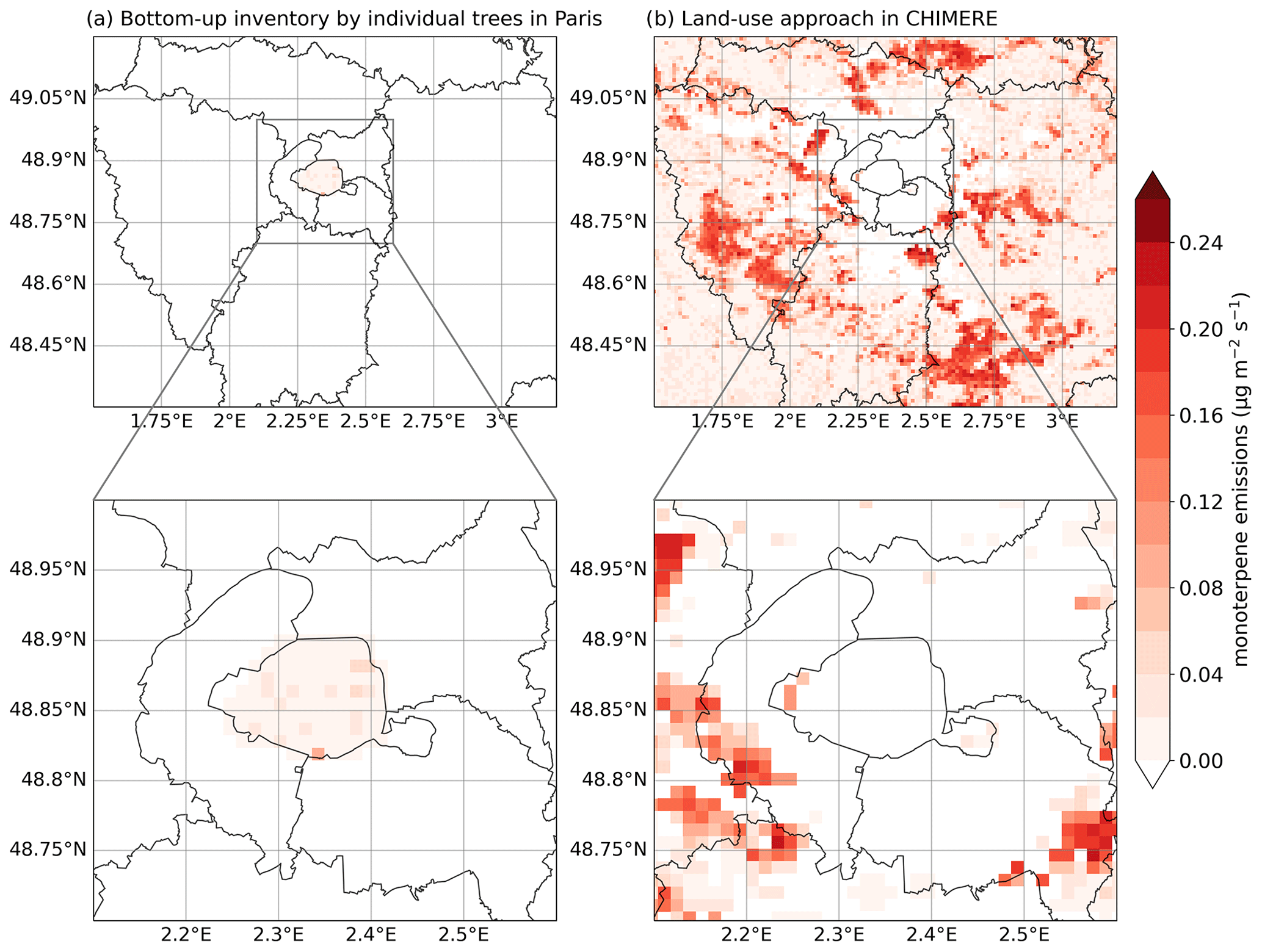
Figure D2 Comparison of the 2-month-averaged monoterpene emissions computed with (a) the bottom-up inventory and (b) with the land cover approach in CHIMERE over Île-de-France and greater Paris.

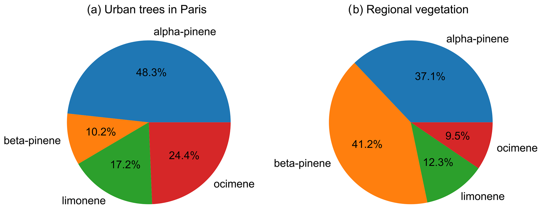
Figure D3 Distribution of monoterpene species emitted and summed over the 2 months (a) for the urban trees in Paris computed with the bottom-up inventory and (b) for the vegetation over Île-de-France region computed with the land use approach.

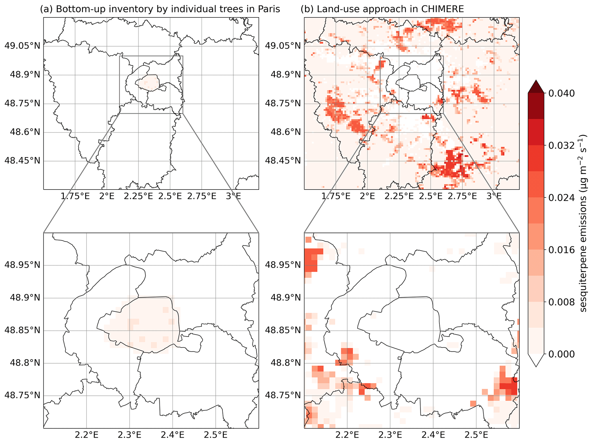
Figure D4 Comparison of the 2-month sesquiterpene emissions computed with (a) the bottom-up inventory and (b) with the land cover approach in CHIMERE over Île-de-France and greater Paris.

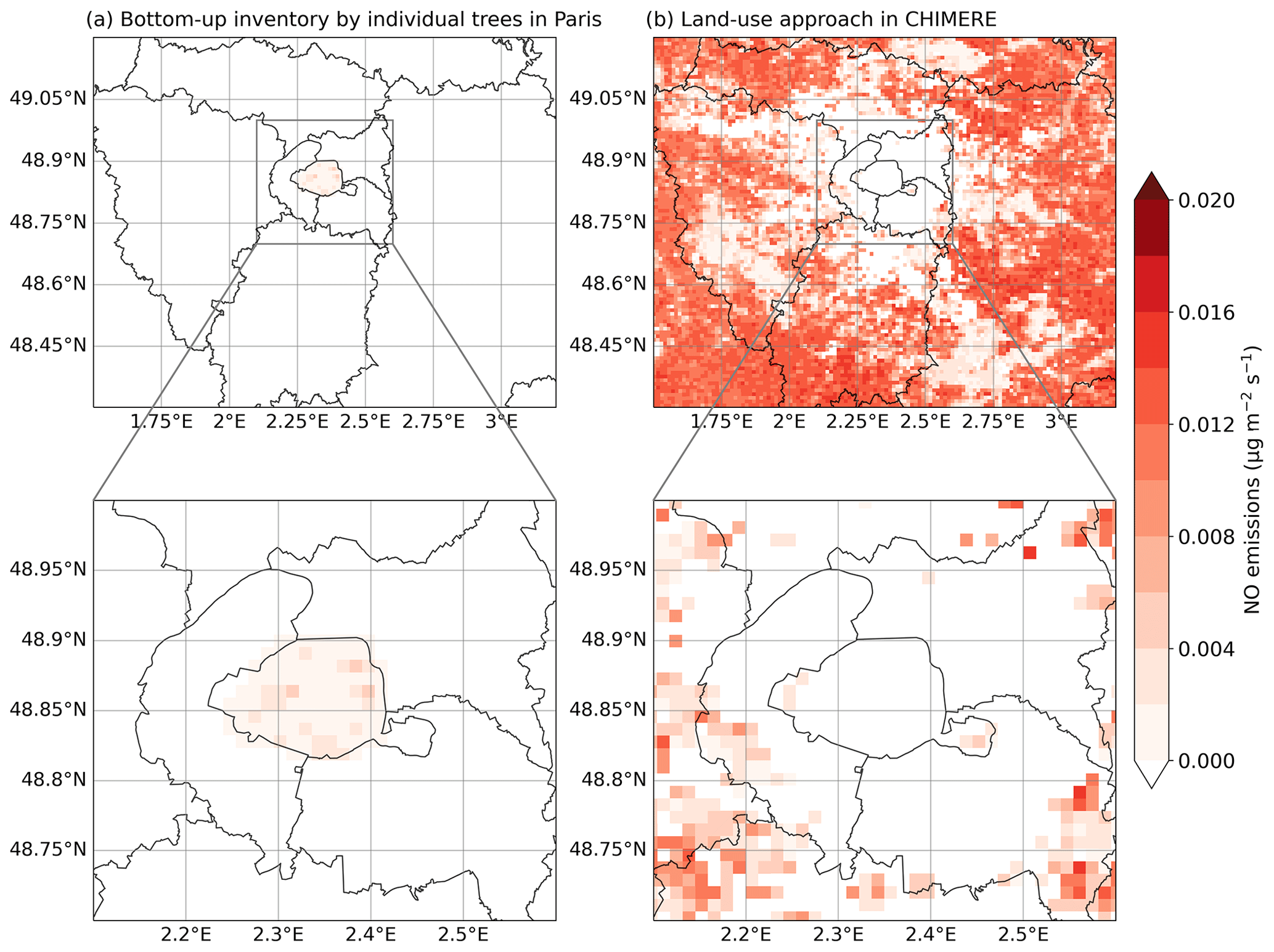
Figure D5 Comparison of the 2-month nitrite oxide (NO) emissions computed with (a) the bottom-up inventory and (b) with the land cover approach in CHIMERE over Île-de-France and greater Paris.

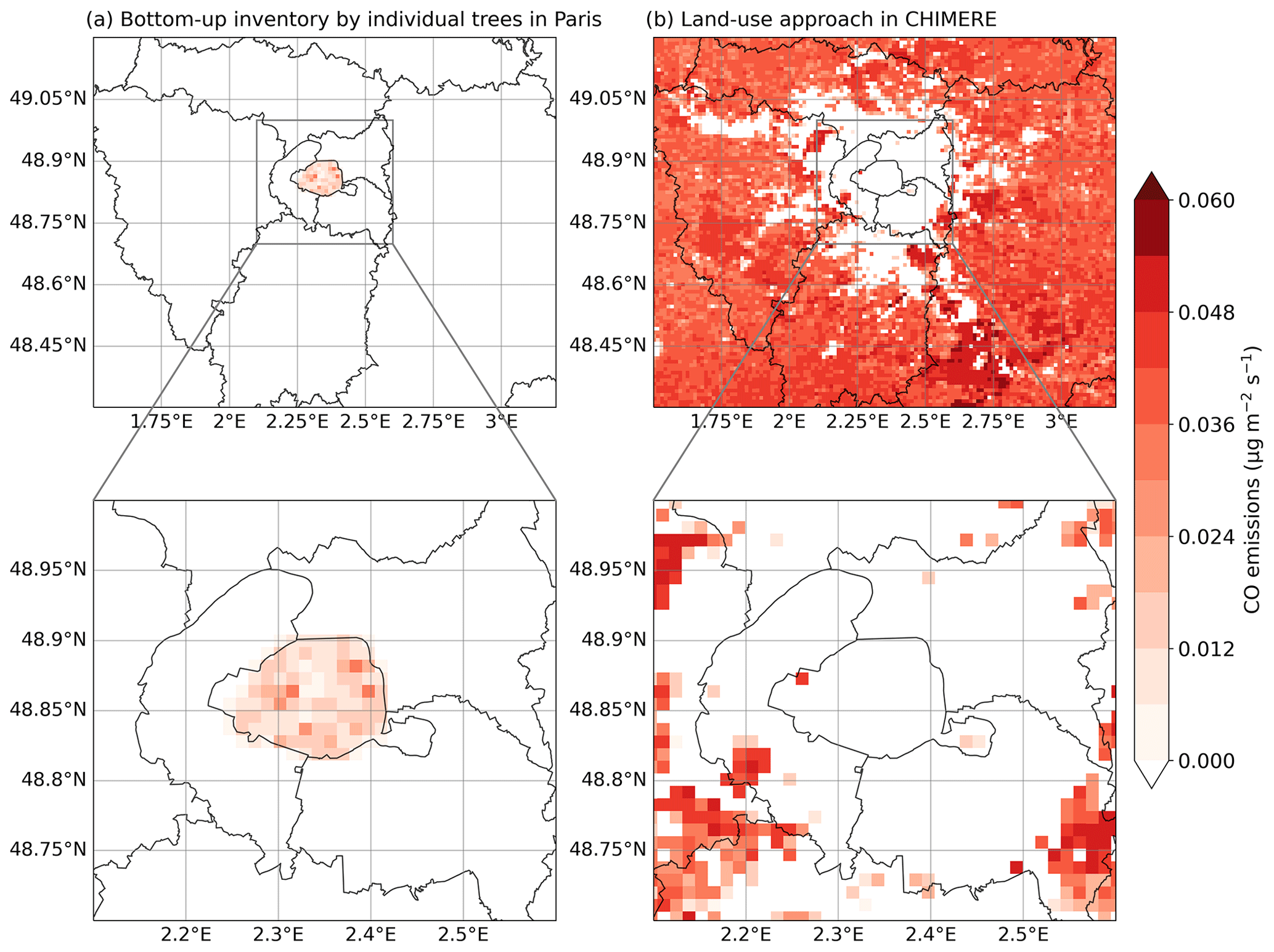
Figure D6 Comparison of the 2-month carbon monoxide (CO) emissions computed with (a) the bottom-up inventory and (b) with the land cover approach in CHIMERE over Île-de-France and greater Paris.

Figure D7 Comparison of the 2-month other VOC (OVOC) emissions computed with (a) the bottom-up inventory and (b) with the land cover approach in CHIMERE over Île-de-France and greater Paris.

Appendix E: Validation of the reference simulations: meteorology

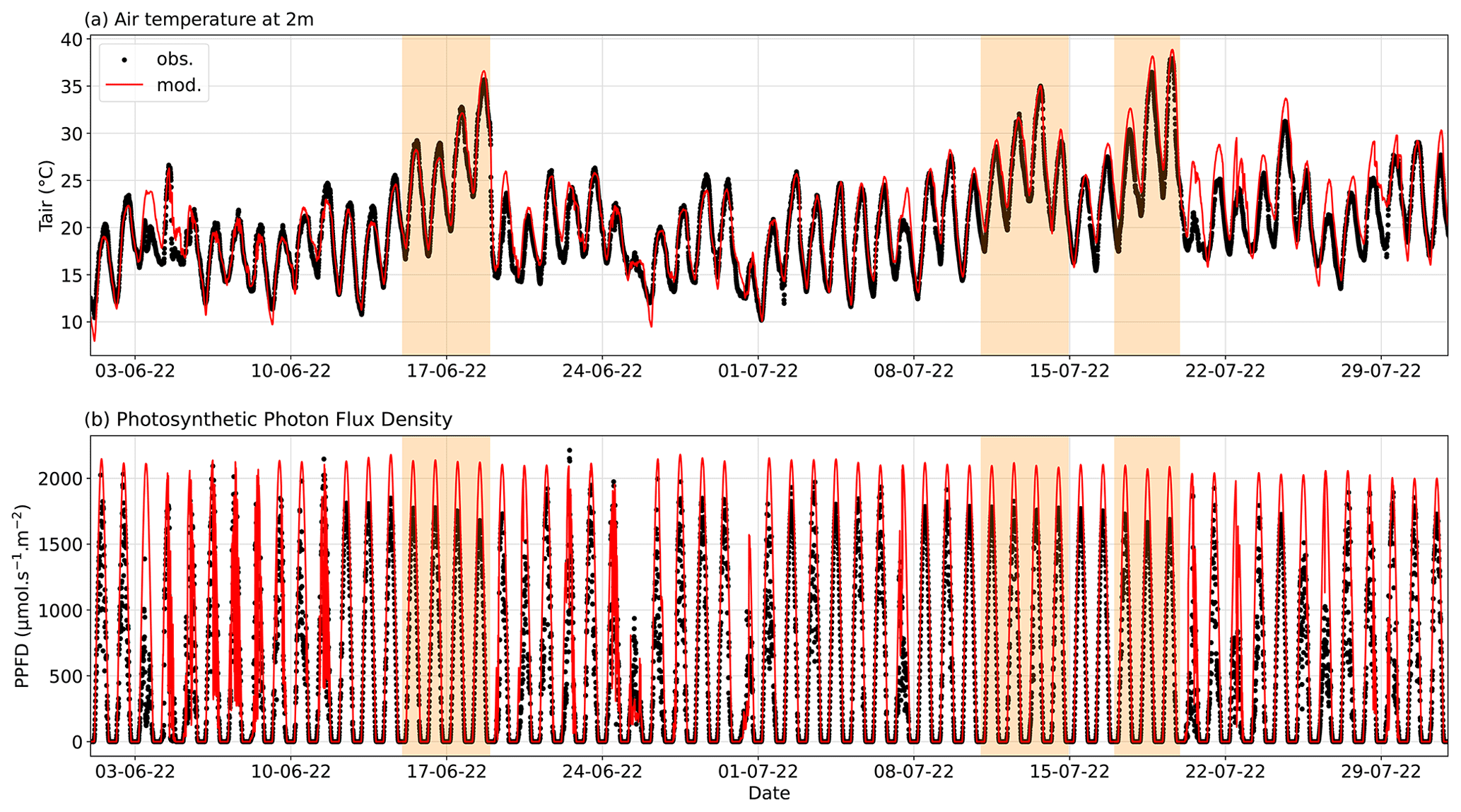
Figure E1 Comparison of the temporal variation in the (a) air temperature at 2 m height and (b) photosynthetic photon flux density modeled by WRF (mod) and observed (obs) at the SIRTA observatory site (48.717347° N, 2.208868° E). Heatwave periods are indicated by shaded orange areas.

This section presents a validation of the surface meteorological fields simulated by WRF-CHIMERE by comparing with measurements performed at SIRTA (Fig. E1 and Table E1) and at seven weather stations operated by Météo-France (Table E2). The meteorological measurements of air temperature (T), relative humidity (RH), pressure (P), precipitation at 2 m, and wind speed and direction at 10 m above ground level, as well as longwave (LW), global shortwave (SW), and PPFD incident radiations at the surface are compared.

The wind speed and direction observed at 10 m are approximated by the value simulated in the grid cell from 0.15 to 24 m that is supposed to represent the field at the mid-cell altitude (i.e., ≈ 12 m). The meteorological fields are extracted from the horizontal cell of the IDF1 domain which includes the station. Figure E1 shows the comparison of modeled and observed air temperature at 2 m height and PPFD, which are the two meteorological variables used to calculate BVOC emissions, from June to July 2022. They are also compared with statistical indicators (defined in Appendix G) in Table E1, along with the other simulated and observed meteorological variables.

Table E1 Statistical indicators for the comparison of the meteorological variables simulated by WRF and observed at the SIRTA observatory site (48.7° N, 2.2° E) at a 10 min time step. RMSE is for root mean square error, NAD is for normalized absolute difference, Bias is for fractional mean bias, R is for Pearson correlation coefficient (Appendix G), a.g.l. is for above ground level, and su is for the same unit as the meteorological variable.

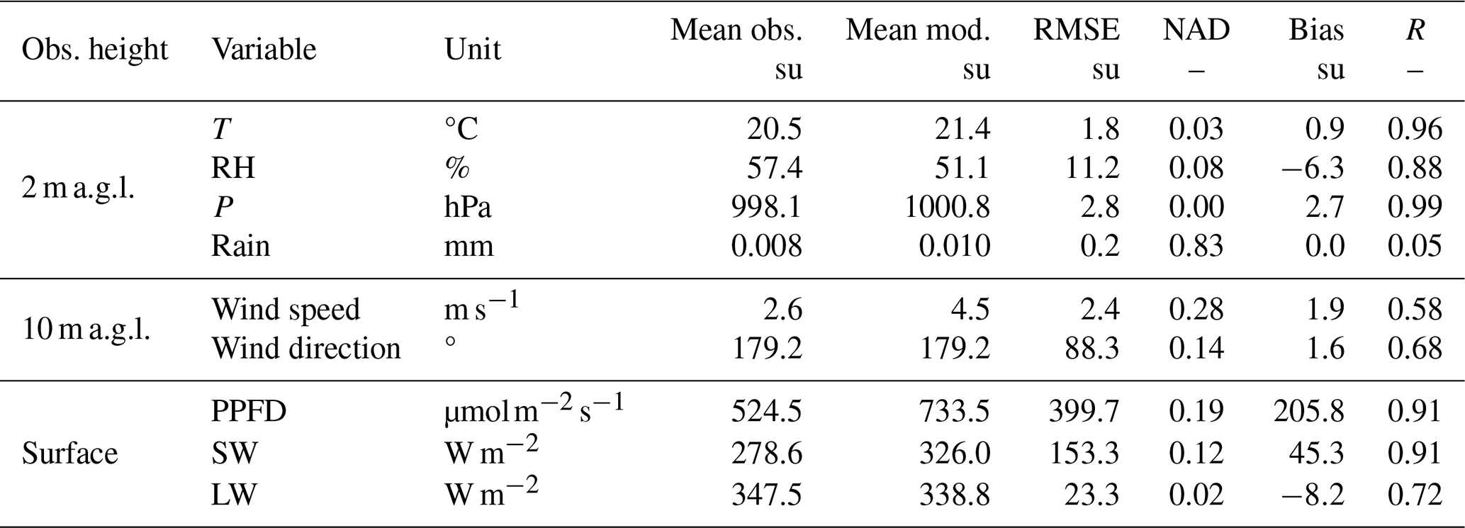
Figure E1 and Table E1 show that the variations in the air temperature at 2 m and PPFD are well modeled, with high correlations and low errors. The temperature is slightly overestimated by the model, especially after 16 July, resulting in an average positive bias of about 1 °C. For PPFD, the daily maximum is overestimated on some days, resulting in a positive bias. As PPFD is computed from the global solar radiation (SW), and the bias on this global solar radiation is lower, this overestimation may also come from the conversion coefficient between PPFD and solar radiation. Some tests have been performed to compare the BVOC emission of the bottom-up inventory calculated with the PPFD $/$ SW ratio measured at SIRTA instead of the ratio used by CHIMERE (2.25) and showed that the impact on BVOC emissions was not significant. Other meteorological variables such as air relative humidity, pressure, wind direction, and incident longwave radiation are also well modeled (Table E1). The wind speed is slightly overestimated, but this may be due to a difference in the representativity between a punctual wind speed measurement and an average value in the 24 m thick vertical cell. The low rainfall intensity limits the significance of statistical indicator calculations, but the temporal comparison (not shown) demonstrates that the rainy days are well represented by the model, but the intensity of heavy rains is underestimated.

Table E2 shows that the comparison of meteorological variables (T, RH, P, SW, and wind speed and direction) at seven Météo-France stations leads to very similar conclusions to the comparison at SIRTA.

Table E2 Statistical indicators for the comparison of the hourly meteorological variables simulated by WRF and observed at seven Météo-France sites (Montsouris (48.8217° N, 2.3378° E), Longchamp (48.8548° N, 2.2337° E), Melun (48.6103° N, 2.6795° E), Trappes (48.7743° N, 2.0098° E), Versailles (48.8033° N, 2.0900° E), Orly (48.7180° N, 2.3970° E), and Roissy (49.0152° N, 2.5343° E)). RMSE is for root mean square error, NAD is for normalized absolute difference, Bias is for fractional mean bias, R is for Pearson correlation coefficient (Appendix G), a.g.l. is for above ground level, and su is for the same unit as the meteorological variable.

Appendix F: Validation of the reference simulations: model to data comparisons of gas and particle concentrations

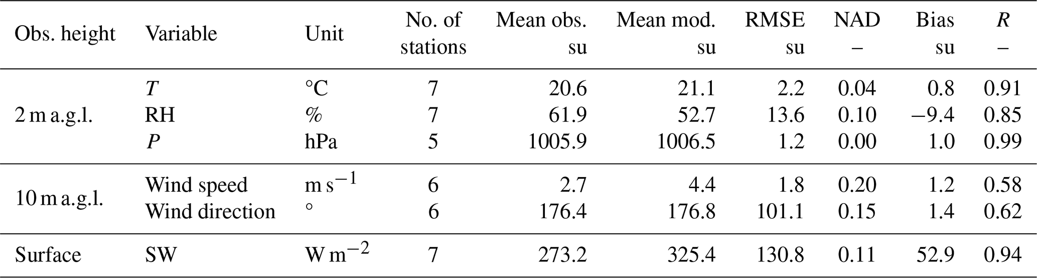
Table F1 Statistical comparison of the observed and simulated concentrations on average over 21 stations in IDF1 (listed in Table A1). Values indicated in bold respect the strictest performance criteria, while those in italics respect the acceptable performance criteria, and those in roman do not respect the performance criteria defined by Hanna and Chang (2012). Correlation coefficients (R) are not included in the performance criteria. FB is for fractional bias, MG is for geometric mean bias, NMSE is for normalized mean square error, VG is for geometric variance, FAC2 is for factor of 2, NAD is for normalized absolute difference, Bias is for fractional mean bias, R is for Pearson correlation coefficient (Appendix G), a.g.l. is for above ground level, and su is for the same unit as the species concentration.

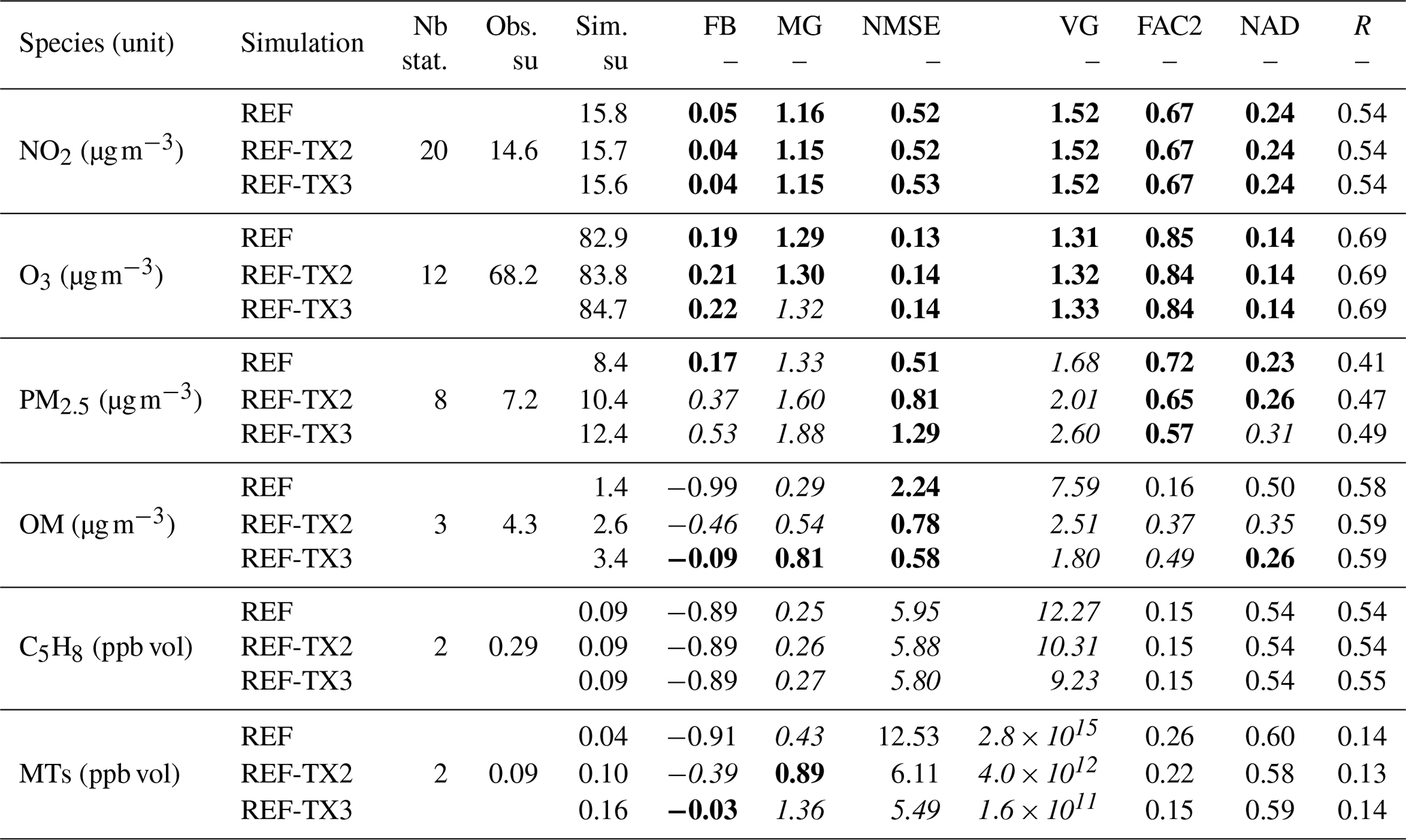
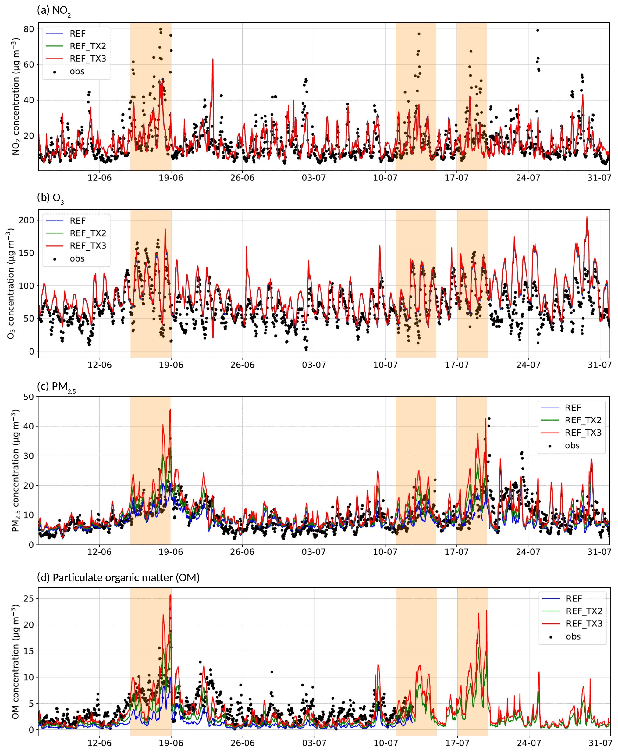
Figure F1 Observed and simulated hourly concentrations of (a) NO₂, (b) O₃, (c) PM_2.5, and (d) OM at the Halles station. Heatwave periods are indicated by shaded orange areas.

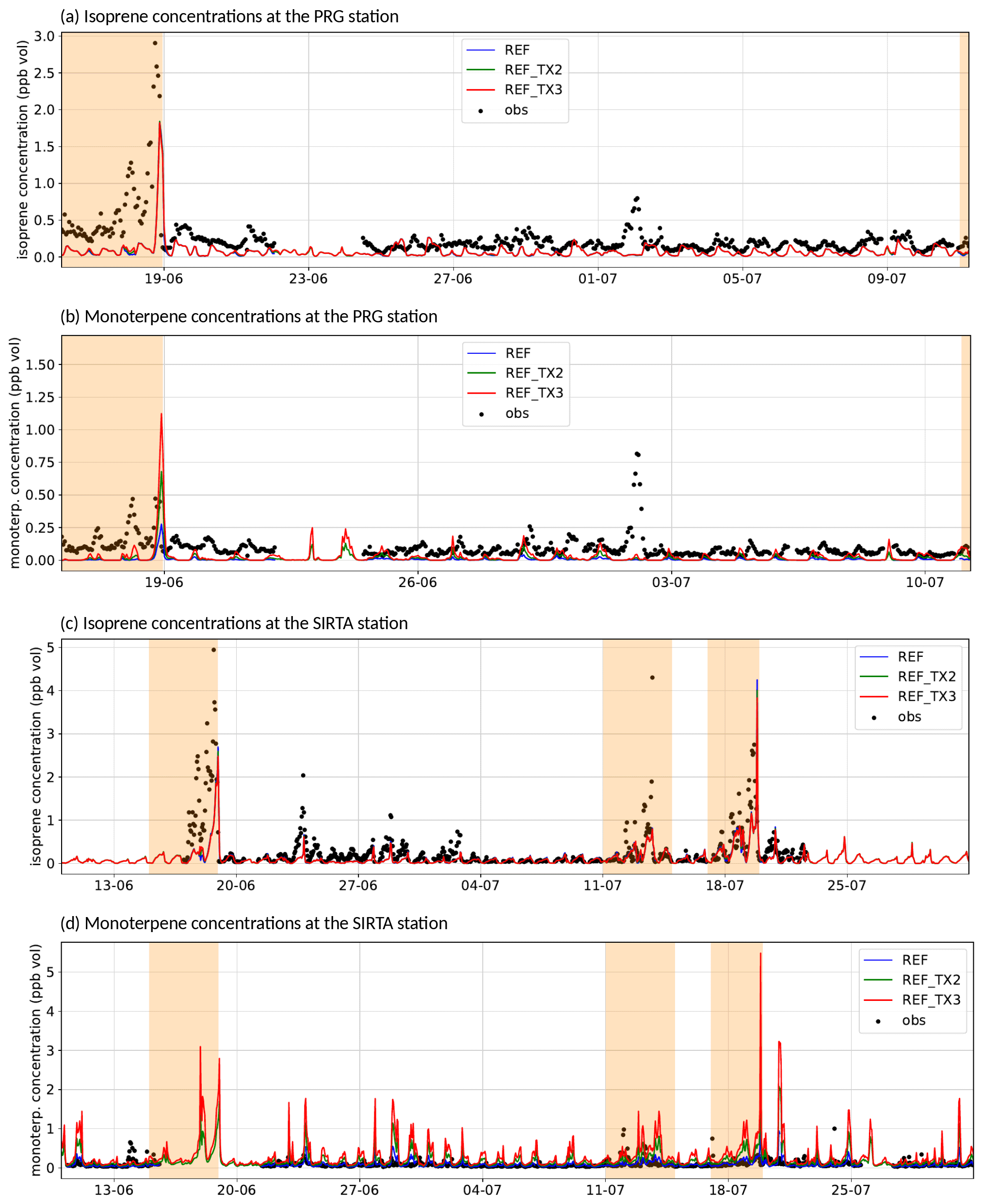
Figure F2 Observed and simulated hourly concentrations of (a) isoprene and (b) monoterpenes at the PRG station and (c) isoprene and (d) monoterpenes at the SIRTA station. Heatwave periods are indicated by shaded orange areas.

In this section, the NO₂, O₃, OM, PM_2.5, and isoprene and monoterpene concentrations simulated by CHIMERE are compared to observations performed at different measurement stations over Île-de-France. The concentrations simulated in the horizontal grid cell containing the station and in the first vertical layer are compared to the observed concentrations in Table F1 for the three emission scenarios REF, REF-TX2, and REF-TX3. Two performance criteria are defined by Hanna and Chang (2012), and they are used here to evaluate the simulations performance. The strictest criteria are accepted when −0.3 < FB < 0.3, 0.7 < MG < 1.3, NMSE < 3, VG < 1.6, FAC2 ≥ 0.5, and NAD < 0.3. The less strict criteria are accepted when −0.67 < FB < 0.67, NMSE < 6, FAC2 ≥ 0.3, and NAD < 0.5 (where FB is for fractional bias, MG is for geometric mean bias, NMSE is for normalized mean square error, VG is for geometric variance, FAC2 is for factor of 2, NAD is for normalized absolute difference, and R is for correlation coefficient; see Appendix G). Values that respect the strictest performance criteria are represented in bold, those that respect the acceptable performance criteria for urban areas are represented in italics, and those that do not respect any criteria are in roman. In order to investigate in more detail the model performance in each simulation, the temporal evolution of simulated and observed concentrations in three different stations (the Halles and PRG urban stations and the SIRTA suburban station) is presented in Figs. F1 and F2.

The different hypotheses regarding terpene biogenic emissions have a low impact on NO₂ and O₃ concentrations, and all simulations present very similar concentrations and statistical indicators (Table F1). Figure F1a shows good correlation between the NO₂ concentrations measured and observed at the Halles site in all simulations, although a few concentration peaks are underestimated. The strictest performance criteria are respected for all statistical indicators for NO₂ and for O₃. The O₃ geometric mean bias is at the limit of the acceptance criteria because of the overestimation of the low O₃ concentrations at night (see Fig. F1b). This overestimation of low O₃ concentrations has previously commonly been observed and might be related to model grid resolution (Jang et al., 1995a, b; Liang and Jacobson, 2000; Arunachalam et al., 2006).

For PM_2.5, the less strict criteria are respected for the three simulations, but the fractional bias (FB) increases with the increase in the biogenic terpene emissions. This increase is observed mostly in rural stations. In other words, PM_2.5 concentrations are overestimated at rural stations when the terpene biogenic emissions are increased, but the increase in the terpene biogenic emissions does not degrade the scores at urban and suburban stations, and it even improves the correlation. A PM_2.5 concentration peak reaching 80 µg m⁻³ is observed on 19 July (not shown in Fig. F1c) and is probably due to forest fires in the southwest of France (Menut et al., 2023). Similar to PM_2.5, the concentrations of the organic fraction of PM₁ (organic matter, OM) are strongly influenced by the terpene biogenic emission hypothesis. While OM concentrations are strongly underestimated in the REF simulation (fractional bias of −0.99), they respect all the less strict criteria in the REF-TX2 and REF-TX3 simulations (fractional bias equal to −0.46 and −0.09, respectively). As the stations where OM is measured are suburban and urban stations, this goes hand in hand with the better estimate of PM_2.5 at urban stations (not shown). As shown in Fig. F1c, the effect of modifying biogenic terpene emissions is quite significant, even at the Halles station, which is located in a very dense urban area. This increase in the PM_2.5 concentrations is due to the increase in OM, as shown in Fig. F1d. OM concentrations are especially high between 18 and 19 June, days with very high temperatures and high biogenic emissions. During this period, the differences between the OM concentrations in the REF, REF-TX2, and REF-TX3 simulations are the largest. The higher the terpene emissions, the better the simulated OM concentration is compared to observation, suggesting that it is essential to represent the terpene emission of suburban areas well to represent the OM concentrations well.

Regarding BVOC concentrations, no differences in the three simulations are observed for isoprene (C₅H₈) concentrations, as expected, and the mean concentration tends to be underestimated. Monoterpene concentrations are highly influenced by the biogenic terpene emissions. The higher the biogenic terpene emissions are, the smaller the fractional biases observed in the simulations will be (−0.91 for REF, −0.39 for REF-TX2, and −0.03 for REF-TX3) (Table F1). Figure F2a and c show the hourly isoprene concentrations simulated and observed at the PRG station (dense urban area) and at the SIRTA station (suburban area), respectively. Isoprene is better represented at SIRTA than at the PRG station because of the absence of biogenic emissions inside Paris in REF, REF-TX2, and REF-TX3 simulations. Figure F2b and d illustrate the hourly concentrations of monoterpenes simulated and observed at the PRG and SIRTA stations, respectively. Similar to what was observed for isoprene, monoterpene concentrations are also strongly underestimated in urban areas (PRG) and are better represented at the SIRTA suburban site. This can be justified by the absence of monoterpene biogenic emissions inside Paris, as analyzed in Sect. 4.2. The observed values in the urban PRG site point out a “regional background” of the monoterpene concentrations around 0.1 ppb.

Appendix G: Definition of the statistical indicators

To compare the simulation results to measured data, classical statistical indicators are computed where obs_i and sim_i are, respectively, the observed and simulated hourly concentrations. n is the total number of concentrations, and $\stackrel{\mathrm{‾}}{\text{obs}}$ and $\stackrel{\mathrm{‾}}{\text{sim}}$ are the average observed and simulated concentrations.

• -

  Root mean square error (same unit as the concentration):

  $$\begin{array}{}\text{(G1)}& \text{RMSE}=\sqrt{{\displaystyle \frac{\mathrm{1}}{n}}\sum _{i=\mathrm{1}}^n{\left({\text{obs}}_i-{\text{sim}}_i\right)}^{\mathrm{2}}}.\end{array}$$
• -

  Normalized mean square error (dimensionless):

  $$\begin{array}{}\text{(G2)}& \text{NMSE}={\displaystyle \frac{\sum _{i=\mathrm{1}}^n{\left({\text{obs}}_i-{\text{sim}}_i\right)}^{\mathrm{2}}}{\sum _{i=\mathrm{1}}^n{\text{obs}}_i\times \sum _{i=\mathrm{1}}^n{\text{sim}}_i}}.\end{array}$$
• -

  Normalized absolute difference (dimensionless):

  $$\begin{array}{}\text{(G3)}& \text{NAD}={\displaystyle \frac{\sum _{i=\mathrm{1}}^n|{\text{obs}}_i-{\text{sim}}_i|}{\sum _{i=\mathrm{1}}^n{\text{obs}}_i+\sum _{i=\mathrm{1}}^n{\text{sim}}_i}}.\end{array}$$
• -

  Mean fractional error (dimensionless):

  $$\begin{array}{}\text{(G4)}& \text{MFE}={\displaystyle \frac{\mathrm{1}}{n}}\sum _{i=\mathrm{1}}^n{\displaystyle \frac{|{\text{sim}}_i-{\text{obs}}_i|}{{\text{obs}}_i}}.\end{array}$$
• -

  Mean fractional bias (same unit as the concentration):

  $$\begin{array}{}\text{(G5)}& \text{MFB}={\displaystyle \frac{\mathrm{1}}{n}}\sum _{i=\mathrm{1}}^n|{\text{sim}}_i-{\text{obs}}_i|.\end{array}$$
• -

  Bias (same unit as the concentration):

  $$\begin{array}{}\text{(G6)}& \text{Bias}={\displaystyle \frac{\mathrm{1}}{n}}\sum _{i=\mathrm{1}}^n\left({\text{sim}}_i-{\text{obs}}_i\right).\end{array}$$
• -

  Fractional bias (dimensionless):

  $$\begin{array}{}\text{(G7)}& \text{FB}=\mathrm{2}\times {\displaystyle \frac{\sum _{i=\mathrm{1}}^n{\text{sim}}_i-\sum _{i=\mathrm{1}}^n{\text{obs}}_i}{\sum _{i=\mathrm{1}}^n{\text{obs}}_i+\sum _{i=\mathrm{1}}^n{\text{sim}}_i}}.\end{array}$$
• -

  Geometric mean bias (dimensionless):

  $$\begin{array}{}\text{(G8)}& \text{MG}=\exp \left[{\displaystyle \frac{\mathrm{1}}{n}}\sum _{i=\mathrm{1}}^n\ln \left({\text{sim}}_i\right)-{\displaystyle \frac{\mathrm{1}}{n}}\sum _{i=\mathrm{1}}^n\ln \left({\text{obs}}_i\right)\right].\end{array}$$
• -

  Correlation coefficient (dimensionless):

  $$\begin{array}{}\text{(G9)}& R={\displaystyle \frac{\sum _{i=\mathrm{1}}^n\left[\left({\text{sim}}_i-\stackrel{\mathrm{‾}}{\text{sim}}\right)\left({\text{obs}}_i-\stackrel{\mathrm{‾}}{\text{obs}}\right)\right]}{\sqrt{\sum _{i=\mathrm{1}}^n{\left({\text{sim}}_i-\stackrel{\mathrm{‾}}{\text{sim}}\right)}^{\mathrm{2}}\sum _{i=\mathrm{1}}^n{\left({\text{obs}}_i-\stackrel{\mathrm{‾}}{\text{obs}}\right)}^{\mathrm{2}}}}}.\end{array}$$
• -

  Geometric variance (dimensionless):

  $$\begin{array}{}\text{(G10)}& \text{VG}=\exp \left[{\displaystyle \frac{\mathrm{1}}{n}}\sum _{i=\mathrm{1}}^n{\left(\ln \left({\text{obs}}_i\right)-\ln \left({\text{sim}}_i\right)\right)}^{\mathrm{2}}\right].\end{array}$$
• -

  Factor of 2 (dimensionless):

  $$\begin{array}{}\text{(G11)}& \text{FAC2}=\text{total fraction where}\mathrm{0.5}<{\displaystyle \frac{{\text{sim}}_i}{{\text{obs}}_i}}<\mathrm{2.0}.\end{array}$$