Cloud response to co-condensation of water and organic vapors over the boreal forest

Accounting for the condensation of organic vapors along with water vapor (co-condensation) has been shown in adiabatic cloud parcel model (CPM) simulations to enhance the number of aerosol particles that activate to form cloud droplets. The boreal forest is an important source of biogenic organic vapors, but the role of these vapors in co-condensation has not been systematically investigated. In this work, the environmental conditions under which strong co-condensation-driven cloud droplet number enhancements would be expected over the boreal biome are identified. Recent measurement technology, specifically the Filter Inlet for Gases and AEROsols (FIGAERO) coupled to an iodide-adduct chemical ionization mass spectrometer (I-CIMS), is utilized to construct volatility distributions of the boreal atmospheric organics. Then, a suite of CPM simulations initialized with a comprehensive set of concurrent aerosol observations collected in the boreal forest of Finland during spring 2014 is performed. The degree to which co-condensation impacts droplet formation in the model is shown to be dependent on the initialization of temperature, relative humidity, updraft velocity, aerosol size distribution, organic vapor concentration, and the volatility distribution. The predicted median enhancements in cloud droplet number concentration (CDNC) due to accounting for the co-condensation of water and organics fall on average between 16 % and 22 %. This corresponds to activating particles 10–16 nm smaller in dry diameter that would otherwise remain as interstitial aerosol. The highest CDNC enhancements (ΔCDNC) are predicted in the presence of a nascent ultrafine aerosol mode with a geometric mean diameter of ∼ 40 nm and no clear Hoppel minimum, indicative of pristine environments with a source of ultrafine particles (e.g., via new particle formation processes). Such aerosol size distributions are observed 30 %–40 % of the time in the studied boreal forest environment in spring and fall when new particle formation frequency is the highest. To evaluate the frequencies with which such distributions are experienced by an Earth system model over the whole boreal biome, 5 years of UK Earth System Model (UKESM1) simulations are further used. The frequencies are substantially lower than those observed at the boreal forest measurement site (< 6 % of the time), and the positive values, peaking in spring, are modeled only over Fennoscandia and the western parts of Siberia. Overall, the similarities in the size distributions between observed and modeled (UKESM1) are limited, which would limit the ability of this model, or any model with a similar aerosol representation, to project the climate relevance of co-condensation over the boreal forest. For the critical aerosol size distribution regime, ΔCDNC is shown to be sensitive to the concentrations of semi-volatile and some intermediate-volatility organic compounds (SVOCs and IVOCs), especially when the overall particle surface area is low. The magnitudes of ΔCDNC remain less affected by the more volatile vapors such as formic acid and extremely low- and low-volatility organic compounds (ELVOCs and LVOCs). The reasons for this are that most volatile organic vapors condense inefficiently due to their high volatility below the cloud base, and the concentrations of LVOCs and ELVOCs are too low to gain significant concentrations of soluble mass to reduce the critical supersaturations enough for droplet activation to occur. A reduction in the critical supersaturation caused by organic condensation emerges as the main driver of the modeled ΔCDNC. The results highlight the potential significance of co-condensation in pristine boreal environments close to sources of fresh ultrafine particles. For accurate predictions of co-condensation effects on CDNC, also in larger-scale models, an accurate representation of the aerosol size distribution is critical. Further studies targeted at finding observational evidence and constraints for co-condensation in the field are encouraged.

1 Introduction

Boreal forests emit significant quantities of volatile organic compounds (VOCs; Guenther et al., 1995; Artaxo et al., 2022), such as monoterpenes that undergo oxidation in the atmosphere. The condensable oxidation products contribute considerably to the secondary organic aerosol (SOA) mass concentrations in the boreal forest air (e.g., Tunved et al., 2006; Artaxo et al., 2022). The emissions of monoterpenes are strongly temperature-dependent, which leads – together with the higher oxidative potential in the sunlit months – to the highest biogenic SOA concentrations in summer (Paasonen et al., 2013; Heikkinen et al., 2020; Mikhailov et al., 2017). This has recently been shown to have implications for cloud properties above the boreal forest through the availability of more cloud condensation nuclei (CCN; Yli-Juuti et al., 2021; Petäjä et al., 2022; Paasonen et al., 2013). Under constant meteorological conditions in the boreal forest, an increase in aerosol concentration typically results in an increase in cloud droplet number concentration (CDNC) and smaller average droplet size for a given liquid water content (Yli-Juuti et al., 2021). These effects alter the cloud brightness, making clouds scatter incoming solar radiation more efficiently (Twomey effect; Twomey, 1974, 1977). The relationships between the number of aerosol particles, CDNC, and their effects on climate are, however, non-linear and complex, which makes aerosol–cloud interactions the largest source of uncertainty in radiative forcing estimates from climate models (e.g., Lohmann and Feichter, 2005; Carslaw et al., 2013; Bellouin et al., 2020). The development of “bottom-up” predictive models is needed for providing accurate, yet robust, simplifications of key processes involved in aerosol–cloud interactions – eventually for inclusion in climate models in computationally efficient parameterizations.

Numerous studies have been carried out to understand the role of condensable organic vapors in SOA formation (e.g., Hallquist et al., 2009; Shrivastava et al., 2017) and hence the concentrations of CCN (i.e., particles of at least 50–100 nm in diameter for the water vapor supersaturations typical of the boreal environments; Cerully et al., 2011; Sihto et al., 2011; Paramonov et al., 2013; Hong et al., 2014; Paramonov et al., 2015). The yields of volatile, intermediate-volatility, or semi-volatile organic compounds (VOCs, IVOCs, or SVOCs) from monoterpene oxidation, such as those of pinonaldehyde, formic acid, or acetic acid, are generally much higher than those of the readily condensable lower-volatility vapors (low-volatility organic compounds, LVOCs, and extremely low-volatility organic compounds, ELVOCs), but they are typically not considered directly important for SOA or CCN formation. The abovementioned volatility classes are determined based on the volatilities of individual compounds binned into a volatility basis set (VBS; Donahue et al., 2006). VOCs have a saturation vapor concentration (C^∗; given in units of µg m⁻³ throughout the paper) of at least 10⁷ µg m⁻³, IVOCs are distributed in the C^∗ range of [10³,10⁶] µg m⁻³, SVOCs of [1,100], LVOCs of $[{\mathrm{10}}^{-\mathrm{3}},{\mathrm{10}}^{-\mathrm{1}}]$, and ELVOCs have a C^∗ below 10⁻⁴ µg m⁻³ (e.g., Donahue et al., 2011). While VOCs, IVOCs, and some SVOCs are unlikely to produce significant concentrations of SOA at ground level without additional oxidation steps or multiphase chemistry, some of them can condense at higher altitudes if transported aloft (e.g., Murphy et al., 2015). In addition, aerosol liquid water plays a key role in determining the number of SVOCs and IVOCs in the condensed phase. Liquid water acts as an absorptive medium, and a higher liquid water content can enable a higher quantity of organic vapors to partition into the condensed phase. However, the role of water in determining partitioning coefficients is often neglected when absorptive partitioning theory (Pankow et al., 2001) is applied. Barley et al. (2009) demonstrated that the inclusion of water, when predicting absorptive partitioning using Raoult's law, could lead to evident increases in organic aerosol (OA) mass concentrations under atmospherically relevant OA loadings. Later work by Topping and McFiggans (2012) showed how, under a decreasing temperature trend, the concentration of aerosol liquid water increases, making the solution particle more dilute and enabling enhanced dynamic partitioning of organic vapors (together with water vapor).

This work focuses on the dynamic SVOC and IVOC condensation, together with water vapor (co-condensation) in rising and cooling air motions, and the effects co-condensation poses on cloud microphysics.

Warm (liquid) clouds can form when air rises and cools, eventually leading to the air being supersaturated with water vapor. The excess water vapor condenses onto aerosol particles, rapidly growing them into cloud droplets. While water represents the most abundant vapor in the atmosphere, other trace species can also influence the cloud droplet activation process as the cooling of the rising air triggers also their condensation. The partitioning of these other vapors into the condensed phase is partially driven by the decrease in temperature itself, which makes the species less volatile, but more important is the increase in aerosol liquid water and the dilution of the aerosol solution that enables them to partition to the liquid phase (Topping and McFiggans, 2012). As the trace vapors condense in the rising air under sub-saturated conditions, the molar fraction of water in the swelling aerosol particles increases slower than in the absence of this co-condensation process, which in turn leads to the condensation of additional water by the time the air parcel reaches the lifting condensation level. The co-condensation of water with other trace vapors eventually leads to a reduction in the critical supersaturation (s^∗) required for droplet activation of the particles due to an increased amount of organic solute (Topping and McFiggans, 2012), as described by Köhler theory (Köhler, 1936). Topping et al. (2013) studied the impact of organic co-condensation on CDNC using a cloud parcel model (CPM) initialized with a suite of realistic conditions describing the aerosol particle number size distribution (PNSD), composition, and OA volatility distribution. They modeled significant enhancements in CDNC (ΔCDNC up to roughly 50 %) when comparing simulations with organic condensation (CC) to simulations without it (noCC). In addition to co-condensing organics and water, co-condensation of nitric acid and ammonia with water has also been suggested to enhance CDNC in earlier process modeling studies (e.g., Kulmala et al., 1993; Korhonen et al., 1996; Hegg, 2000; Romakkaniemi et al., 2005). Direct experimental studies of co-condensation remain challenging, however, as aerosol particles are typically dried during the sampling process, and the loss of liquid water may lead to evaporation of co-condensed organics too. While direct observational evidence of co-condensation is scarce, recent laboratory studies show significant water uptake due to co-condensation of propylene glycol and water onto ammonium sulfate particles (Hu et al., 2018). In addition, ambient observations from Delhi and Beijing suggest the co-condensation of hydrochloric acid (HCl) or nitric acid (HNO₃) with water vapor, respectively, to be essential for reproducing particle hygroscopicities corresponding to the visibility measurements during haze events (Gunthe et al., 2021; Wang et al., 2020).

The cloud response to co-condensation in the form of ΔCDNC has been previously shown to result from the complex interplay between updraft velocity, PNSD, and organic compound volatility distribution (Topping et al., 2013). For the same amount of organic vapor, Topping et al. (2013) found a non-linear response of ΔCDNC to changing updraft velocity. The highest ΔCDNC were obtained when updrafts were below 1 m s⁻¹, but the peak ΔCDNC was dependent on the initial PNSD characteristics. Under higher updrafts, the modeled ΔCDNC was found to decrease exponentially as a function of updraft, but the plateau of the curve depended on the initial PNSD – although the dependence on the exact parameters describing multimodal PNSD were not extensively explored. If assumed representative of the global continents, ΔCDNC values of tens of percent could impose a significant impact on predictions of cloud albedo and the Earth's radiative budget. In fact, Topping et al. (2013) suggest accounting for co-condensation could result in up to 2.5 % increase in cloud albedo (corresponding to global ΔCDNC = 40 %). This albedo increase would translate into a −1.8 W m⁻² change in the global cloud radiative effect over land. Topping et al. (2013) stress, however, that the impacts of co-condensation will be spatially heterogeneous because of variable surface albedo and variation in VOC sources. For comparison, one should note that the net radiative effect of clouds is approximately −20 W m⁻² (Boucher et al., 2013). The recent best estimate of the effective radiative forcing from aerosol–cloud interactions is, on the other hand, −1.0 [−1.7 to −0.3] W m⁻² (Forster et al., 2021). The potential contribution of co-condensation to estimates of radiative forcing due to aerosol–cloud–climate feedbacks remains unclear.

Boreal forests make up about one-third of the Earth's forested area, which makes the boreal biome an important source of biogenic organic vapors that could affect droplet activation in warm clouds through co-condensation. ΔCDNC due to co-condensation over the boreal forest could reduce the albedo over the dark boreal forest canopy. In a warming climate, temperature-dependent biogenic terpene emissions (Guenther et al., 1993) are expected to rise (e.g., Turnock et al., 2020). These increasing emissions enrich the ambient pool of organics available for condensation in rising air. As suggested in Topping et al. (2013), through the effects organic co-condensation pose on CDNC, organic co-condensation could enhance the proposed negative climate feedback mechanism associated with the biogenic SOA (Kulmala et al., 2004; Spracklen et al., 2008; Kulmala et al., 2014; Yli-Juuti et al., 2021), the magnitude of which is currently highly uncertain (Thornhill et al., 2021; Sporre et al., 2019; Scott et al., 2018; Paasonen et al., 2013; Sporre et al., 2020).

Since the publication of the Topping et al. (2013) study, improved constraints of the effective volatilities of organic aerosol (e.g., Thornton et al., 2020) are available through the application of chemical ionization mass spectrometers (CIMS), providing molecular level information on gas- and particle-phase composition in near-real time. With the up-to-date volatility parameterizations using the molecular formulae retrieved from CIMS data, volatility distributions can be calculated along a volatility scale ranging from ELVOCs to VOCs, while previous techniques could not enable constraints on volatilities exceeding $C^{\ast }=$ 1000 µg m⁻³ (Cappa and Jimenez, 2010). This means that a notable amount of semi- and intermediate-volatility vapors with high co-condensation potential were not included in the early organic co-condensation work (Topping et al., 2013; Crooks et al., 2018). The recent methodological developments motivate revisiting work of Topping et al. (2013), as potentially large concentrations of condensable organic vapors have been neglected so far.

In this study, the cloud response to the co-condensation of organic vapors over the boreal forest of Finland is investigated using a CPM. Measurements and parameterization techniques involving Filter Inlet for Gases and AEROsols (FIGAERO)-I-CIMS data are utilized to constrain the volatility distribution of organics for these simulations. In addition, to ensure realistic modeling scenarios, simultaneously recorded measurements of PNSD and chemical composition from the aerosol chemical speciation monitor (ACSM) are used for the CPM initialization. In total, 97 unique CPM simulations are performed, initialized with conditions from boreal spring and early summer, following measurement time series recorded during the Biogenic Aerosols – Effects on Clouds and Climate (BAECC) campaign at the Station for Measuring Atmosphere–Ecosystem Relations (SMEAR) II (Hari and Kulmala, 2005) in Finland (Petäjä et al., 2016), and the sensitivity to meteorological conditions is studied. These simulations are then used to characterize the environmental conditions (with respect to the size distribution and organic aerosol volatility distribution characteristics) that promote co-condensation-driven CDNC enhancements in the boreal atmosphere. The frequencies to which a strong cloud response to co-condensation could be expected, and its potential spatiotemporal variability over the boreal biome is further investigated using long-term measurements from SMEAR II station and UK Earth System Model (UKESM1) simulations.

2 Methods and data

This section covers the description of the main modeling tools and measurement data used in this work involving the description of the CPM utilized (Sect. 2.1), the CPM initialization and simulation setup (Sect. 2.2.), and CPM input data measurements and data processing, with independent sections dedicated to the retrievals of volatility distributions for atmospheric organics (Sect. 2.3 and sections therein). The final section is dedicated for describing the UKESM1 simulations (Sect. 2.4).

2.1 The adiabatic cloud parcel model (PARSEC–UFO)

The base of the CPM chosen for this study is the Pseudo-Adiabatic bin-micRophySics university of Exeter Cloud parcel model (PARSEC). It was developed based on the Institute for Marine and Atmospheric research Utrecht (IMAU) pseudo-adiabatic CPM (ICPM, Roelofs and Jongen, 2004; Roelofs, 1992a, b) to allow for simulation of both pseudo-adiabatic and adiabatic ascents of air parcels (Partridge et al., 2011, 2012), as well as numerous optimizations to reduce simulation computational costs, such as a variable time-stepping scheme option for the dynamics and microphysics. PARSEC simulates the condensation and evaporation of water vapor on aerosol particles, particle activation to cloud droplet, unstable growth, collision and coalescence between droplets, and entrainment. In all simulations performed in this study, PARSEC is used in adiabatic ascent configuration, and the fixed time-stepping option in PARSEC is employed.

The model can be initialized with aerosol populations consisting of one or more internal or external mixtures of sulfuric acid, ammonium bisulfate, ammonium sulfate, OA, black carbon, mineral dust, and sea salt. The PNSD are presented in a moving-center binned microphysics scheme comprising 400 size bins between 2 nm and 5 µm in dry radii, which are constructed at model initialization from the three parameters describing log-normal size distributions for the i number of modes – the geometric mean diameter (D_i), the total mode number concentration (N_i), and the geometric standard deviation (σ_i). The model can be initialized with up to four log-normal aerosol modes. PARSEC further provides time evolutions of key thermodynamic and microphysical parameters (e.g., the air parcel temperature (T), pressure (p), supersaturation (s), altitude (z), and the aerosol particle and hydrometeor size distributions).

The dynamical equations used in PARSEC to simulate the adiabatically ascending air parcel equations are the same as those presented by Lee and Pruppacher (1977), where the vertical parcel displacements are determined by the updraft velocity (w, set to a fixed positive constant value in the PARSEC simulations):

$$\begin{array}{}\text{(1)}& {\displaystyle \frac{\mathrm{d}z}{\mathrm{d}t}}=w.\end{array}$$

The changes in pressure are calculated assuming hydrostatic balance, and the temperature decrease along the ascent follows the dry adiabatic lapse rate while also accounting for the latent heat release due to condensation:

$$\begin{array}{}\text{(2)}& {\displaystyle \frac{\mathrm{d}T}{\mathrm{d}t}}={\displaystyle \frac{gw}{c_{\mathrm{p},\mathrm{a}}}}+{\displaystyle \frac{L_{\mathrm{e}}}{c_{\mathrm{p},\mathrm{a}}}}{\displaystyle \frac{\mathrm{d}{x}_{\mathrm{v}}}{\mathrm{d}t}}+{\mathit{\mu }}_J\left[{\displaystyle \frac{L_{\mathrm{e}}}{c_{\mathrm{p},\mathrm{a}}}}\left(x_{\mathrm{v}}-x_{\mathrm{v}}^{\prime }\right)+\left(T+T^{\prime }\right)\right]w,\end{array}$$

where g is the acceleration of gravity, L_e is the latent heat of evaporation, c_p,a is the specific heat capacity of air, and x_v is the water vapor mixing ratio of the air parcel. μ_J is the entrainment rate describing the mixing of the parcel air with environmental air characterized with $x_{\mathrm{v}}^{\prime }$ and T^′. The water vapor mixing ratio in the air parcel changes with the evolving ambient supersaturation:

$$\begin{array}{}\text{(3)}& {\displaystyle \frac{\mathrm{d}s}{\mathrm{d}t}}={\displaystyle \frac{p}{\mathit{\epsilon }{e}_{\mathrm{s}}}}{\displaystyle \frac{\mathrm{d}{x}_{\mathrm{v}}}{\mathrm{d}t}}-\left(\mathrm{1}+s\right)\left[{\displaystyle \frac{\mathit{\epsilon }{L}_{\mathrm{e}}}{R_{\mathrm{a}}{T}^{\mathrm{2}}}}{\displaystyle \frac{\mathrm{d}T}{\mathrm{d}t}}+{\displaystyle \frac{g}{R_{\mathrm{a}}T}}w\right],\end{array}$$

where $\mathit{\epsilon }=R_{\mathrm{a}}/R_{\mathrm{v}}=M_{\mathrm{w}}/M_{\mathrm{a}}=$ 0.622; i.e., the ratio between the specific gas constants for air and water vapor, respectively, or alternatively the molecular weight of water and air, respectively. e_s is the saturation vapor pressure of water. To solve the ordinary differential equations (Eqs. 2–3), the time derivative of the water vapor mixing is approximated as

$$\begin{array}{}\text{(4)}& {\displaystyle \frac{\mathrm{d}{x}_{\mathrm{v}}}{\mathrm{d}t}}\approx -{\displaystyle \frac{\mathrm{\Delta }{x}_{\mathrm{L}}}{\mathrm{\Delta }t}}-{\mathit{\mu }}_J\left(x_{\mathrm{v}}-x_{\mathrm{v}}^{\prime }+x_{\mathrm{L}}\right)w,\end{array}$$

where Δt is the model time step (0.1 s), and the liquid water mixing ratio (x_L) is calculated as a sum of the liquid water mixing ratio across all 400 size bins (index i) for each assigned mode composition (index j):

$$\begin{array}{}\text{(5)}& \mathrm{\Delta }{x}_{\mathrm{L}}={\displaystyle \frac{\mathrm{4}\mathit{\pi }{\mathit{\rho }}_{\mathrm{w}}}{\mathrm{3}{\mathit{\rho }}_{\mathrm{a}}}}\sum _{i=\mathrm{1}}^{n_{\mathrm{a}}}\sum _{j=\mathrm{1}}^{n_{\mathrm{b}}}{n}_{ij}\left(r_{ij}^{\mathrm{3}}-r_{ij,\mathrm{dry}}^{\mathrm{3}}\right),\end{array}$$

where ρ_w is the density of water, ρ_a is the density of dry air, n_ij is the number of particles within size bin i and composition j, and, finally, r_ij and r_ij,dry are the wet and dry radii of the particles, respectively. The wet radii and hence also the particle masses (m) change as water condenses onto the particle (indices dropped for simplicity):

$$\begin{array}{}\text{(6)}& {\displaystyle \frac{\mathrm{d}m}{\mathrm{d}t}}=\mathrm{4}\mathit{\pi }{\mathit{\rho }}_{\mathrm{w}}{r}^{\mathrm{2}}{\displaystyle \frac{\mathrm{d}r}{\mathrm{d}t}}={\displaystyle \frac{\mathrm{4}\mathit{\pi }{\mathit{\rho }}_{\mathrm{w}}r\left(S-S_{\mathrm{eq}}\right)}{\frac{{\mathit{\rho }}_{\mathrm{w}}RT}{{\text{DIFF}}_{\mathrm{v}}^{\ast }{e}_{\mathrm{s}}}+\frac{L_{\mathrm{e}}{\mathit{\rho }}_{\mathrm{w}}}{kT}\left(\frac{L_{\mathrm{e}}}{RT}-\mathrm{1}\right)}},\end{array}$$

where k is the thermal conductivity of air, and DIFF${}_{\mathrm{v}}^{\ast }$ is size-dependent water vapor diffusivity (from Pruppacher and Klett, 1997). Equation (6) is approximated within PARSEC using a linearized form of the condensation equation (Hänel, 1987). Finally, S is the ambient saturation ratio ($S=s+\mathrm{1}$), and S_eq ($S_{\mathrm{eq}}=\text{RH}/\mathrm{100}\mathit{\%}$) is the equilibrium saturation ratio over the (spherical) wet particle surface, the difference of which determines the quantity of excess vapor for the diffusional growth of the particle. While S depends on the updraft source and condensation sink (Eq. 3), S_eq depends on the particle wet radius and composition, and it can be calculated using the Köhler equation (Köhler, 1936), traditionally expressed as

$$\begin{array}{}\text{(7)}& S_{\mathrm{eq}}={\displaystyle \frac{e}{e_{\mathrm{s}}}}=a_{\mathrm{w}}\exp \left({\displaystyle \frac{\mathrm{2}{M}_{\mathrm{w}}\mathit{\gamma }}{RT{\mathit{\rho }}_{\mathrm{w}}r}}\right),\end{array}$$

where e is the partial vapor pressure of water in equilibrium, a_w is the water activity, γ is the droplet surface tension (assumed to be that of water; see Table 1), R is the universal gas constant, T is the droplet temperature, and r is the droplet radius. Assuming dilute droplets, Eq. (7) is approximated in PARSEC for the equilibrium supersaturation ratio as follows (Hänel, 1987):

$$\begin{array}{}\text{(8)}& S_{\mathrm{eq}}\approx \exp \left({\displaystyle \frac{A}{r}}-{\displaystyle \frac{B}{{\left(\frac{r}{r_{\mathrm{dry}}}\right)}^{\mathrm{3}}-\mathrm{1}}}\right),\end{array}$$

where

$$\begin{array}{}\text{(9)}& A={\displaystyle \frac{\mathrm{2}{M}_{\mathrm{w}}\mathit{\gamma }}{RT{\mathit{\rho }}_{\mathrm{w}}}},\end{array}$$

and

$$\begin{array}{}\text{(10)}& B={\displaystyle \frac{{\mathit{\varphi }}_{\mathrm{s}}{M}_{\mathrm{w}}{\mathit{\epsilon }}_{\mathrm{v}}{\mathit{\rho }}_{\mathrm{s}}\mathit{\nu }}{M_{\mathrm{s}}{\mathit{\rho }}_{\mathrm{w}}}}.\end{array}$$

A and B in Eqs. (9) and (10) are the Köhler coefficients, where M_w is the molecular weight of water (g mol⁻¹), M_s refers to the molar mass of the soluble fraction, ρ_w is the density of water (g m⁻³), ϕ_s is the osmotic coefficient of salt in the solution (ϕ_s≈ 1 in ideal solutions), ν is the dissociation constant, and ρ_s and ε_v are the density and the volume fraction of the soluble mass in the aerosol particle, respectively. The dissociation constant is calculated as $\mathit{\nu }=\left({\sum }_i{c}_i^{+}+{\sum }_j{c}_j^{-}\right)/{\sum }_{ij}{c}_{ij}$, where $c_i^{+}$ and $c_j^{-}$ are the concentrations of positive and negative ions, and c_ij is the concentration (mol L⁻¹) of the electrolytes in solution. For detailed descriptions of the B term, the reader is directed to Roelofs (1992a).

Table 1 Overview of the PARSEC–UFO simulation input parameters that remain unchanged in all of the simulation sets conducted with or without co-condensation. The updraft velocities, organic volatility distributions, and organic vapor concentrations that change between simulation sets are reported in Table 2, together with the median model outputs. The time series of these model input data are shown in Fig. 1. All the modeling scenarios are initiated at 90 % relative humidity.

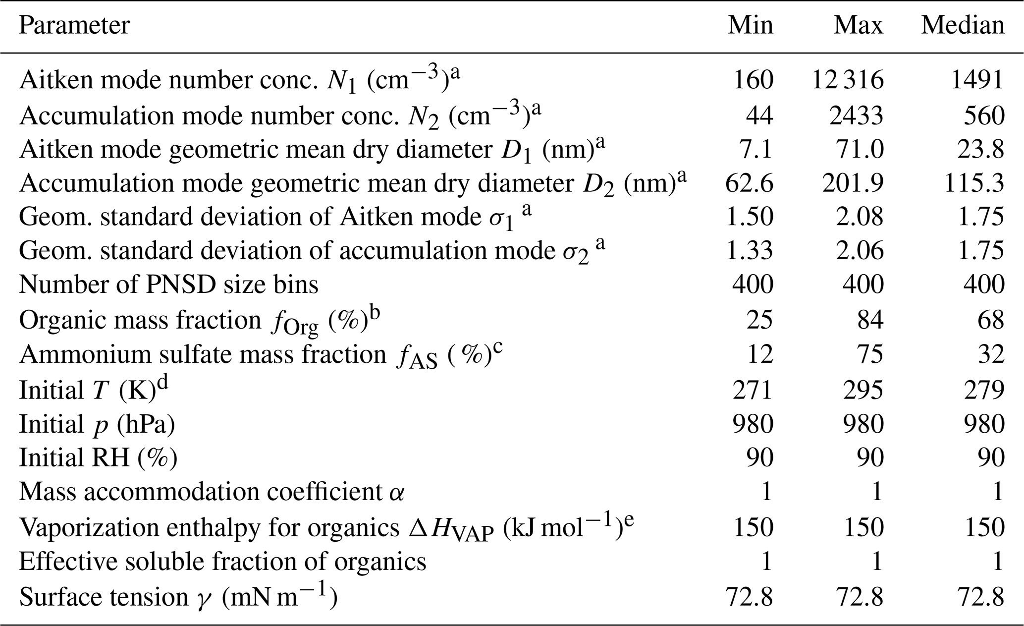
^a Retrieved from fits assigned onto the measured aerosol size distributions (Aalto et al., 2001) using a fitting algorithm by Hussein et al. (2005).
^b Retrieved from aerosol chemical composition measurements (Heikkinen et al., 2020).
^c $f_{\mathrm{AS}}=\mathrm{1}-f_{\mathrm{Org}}$
^d Retrieved from radio soundings (ARM Data Center, 2014). The temperatures shown were recorded when the relative humidity (RH) measured by the radiosonde reached 90 %, i.e., the initial relative humidity used for the adiabatic ascents.
^e Note that in the volatility distribution construction (offline from PARSEC), the ΔH_VAP is temperature-adjusted, following Epstein et al. (2010).

Table 2 Overview of the PARSEC–UFO simulation output for the no co-condensation (noCC) and co-condensation (CC with F volatility distribution) simulations performed using varying updraft velocities provided in the first row of the table.

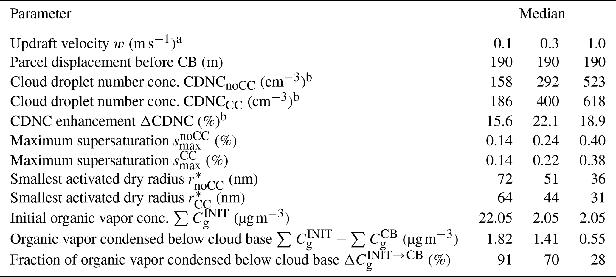
^a Model input parameters crucial for understanding the differences between the co-condensation simulation model outputs.
^b The CDNC represents the integrated number concentration in size bins exceeding the critical radius in wet size at 50 m above cloud base (CB).

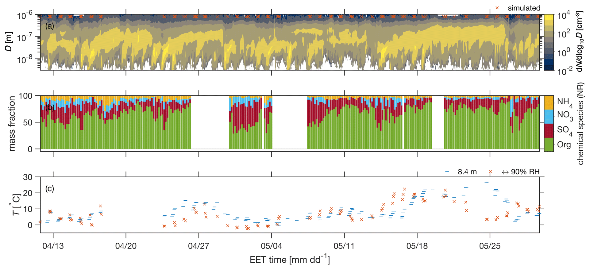
Figure 1 (a) Time series of the particle number size distribution in the time period of interest during BAECC. The time points used for the PARSEC–UFO initialization are shown as red/orange crosses. (b) The non-refractory (NR) chemical composition of sub-micrometer aerosol particles for the same time period. (c) The time series of ambient temperature above ground level (8.4 m a.g.l.) is shown in blue, and the PARSEC–UFO initialization temperature corresponding to RH = 90 % from the interpolated radiosonde data product is shown in orange. The sub-panels have a common x axis representing eastern European winter time (UTC+2).

PARSEC has been further extended to include Köhler and condensation/evaporation equations for organic species of varying volatilities (Lowe, 2020). This extension of the model is referred to as PARSEC with the Unified Framework for Organics (PARSEC–UFO), and it is the CPM version used throughout the presented study. Within PARSEC–UFO, the volatility distributions are given using the VBS framework (Donahue et al., 2006) with q volatility bins – each assigned with a different saturation vapor concentration, C^∗. The condensation$/$evaporation equation for organic species is described in the same manner as in Topping et al. (2013) and as shown for water vapor in Eq. (6):

$$\begin{array}{}\text{(11)}& {\displaystyle \frac{\mathrm{d}{m}_q}{\mathrm{d}t}}={\displaystyle \frac{\mathrm{4}\mathit{\pi }{\mathit{\rho }}_{\mathrm{w}}r{\text{DIFF}}_{\mathrm{g}}^{\ast }\left(S_q-S_{\mathrm{eq},q}\right)e_{\mathrm{s},q}}{\frac{{\text{DIFF}}_{\mathrm{g}}^{\ast }\mathrm{\Delta }{H}_{\mathrm{VAP},q}{S}_{\mathrm{eq},q}{e}_{\mathrm{s},q}{\mathit{\rho }}_q}{\mathit{\lambda }T}\left(\frac{\mathrm{\Delta }{H}_{\mathrm{VAP},q}}{R_{\mathrm{v},\mathrm{q}}T}-\mathrm{1}\right)+{\mathit{\rho }}_q{R}_{\mathrm{v},q}T}},\end{array}$$

where DIFF${}_{\mathrm{g}}^{\ast }$ is the gas-phase diffusivity (see details in Topping et al., 2013, their Supplement), and λ is the heat conductivity of air. Both DIFF${}_{\mathrm{g}}^{\ast }$ and λ are corrected for the transition regime of condensation. ΔH_VAP,q is the enthalpy of vaporization, e_s,q is the saturation vapor pressure, S_eq,q is the equilibrium saturation ratio, and ρ_q is the density of organic species in the qth volatility bin. S_eq,q is calculated analogous to the Köhler equation (Eq. 8):

$$\begin{array}{}\text{(12)}& S_{\mathrm{eq},q}=a_q\exp \left({\displaystyle \frac{\mathrm{2}{\mathit{\upsilon }}_q\mathit{\gamma }}{RTr}}\right),\end{array}$$

where a_q is the activity of qth volatility bin in the bulk condensed phase, which equals the molar fraction of q due to the ideal solution approach of the study, and υ_q is the molar volume of q. Following the organic condensation, the Köhler B term (Eq. 10) is updated along the adiabatic ascent, which impacts S_eq for water and thereby its condensation. Finally, as temperature decreases along the parcel's adiabatic ascent, the reductions in C^∗ are accounted for using an Arrhenius-type Clausius–Clapeyron relation:

$$\begin{array}{}\text{(13)}& C^{\ast }=C^{\ast }\left(T_{\mathrm{ref}}\right)\exp \left({\displaystyle \frac{\mathrm{\Delta }{H}_{\mathrm{VAP}}}{R}}\left({\displaystyle \frac{\mathrm{1}}{T_{\mathrm{ref}}}}-{\displaystyle \frac{\mathrm{1}}{T}}\right)\right),\end{array}$$

where R is the universal gas constant, T is the air parcel's ambient temperature in kelvin, and T_ref is 298.15 K. The C^∗(T_ref) are calculated within PARSEC–UFO using the initial conditions as reference. ΔH_VAP remain constant throughout the simulations in this study and are not C^∗-dependent for simplicity. It should be noted that the time step of 0.1 s can be too high for solving Eq. (11) for the highest-volatility bins. For instance, during condensation, the model may encounter $m_q+\frac{\mathrm{d}{m}_q}{\mathrm{d}t}<\mathrm{0}$.

If this happens, then the condensation step is rejected, and instead condensation happens with a temporary time step of $\mathrm{d}t/\mathrm{2}$ across two iterations. This ensures non-negative m_q. We should stress that this sub-time step is a new feature unique to PARSEC–UFO which is different to the updraft-dependent variable time-stepping scheme option available in PARSEC.

2.2 PARSEC–UFO initialization and simulation setup

The simulations shown within this work are performed with PARSEC–UFO with or without co-condensation. Initially, before the start of the adiabatic ascent, an initialization takes place in PARSEC–UFO. This involves the calculation of the binned wet particle number size distribution and, in the case where co-condensation is enabled, the initialization of the volatility distribution of organics. The binned wet PNSD is calculated using the parameters describing a dry log-normal PNSD (N_i, D_i, σ_i), information on aerosol chemical composition (mass fractions of chemical species), initial RH, and temperature – all given as inputs for the model. When co-condensation is turned on, PARSEC–UFO takes in the summed volatility distributions (gas + particle phase; i.e., $C_{\mathrm{g}+\mathrm{p},q}=C_{\mathrm{g},q}+C_{\mathrm{p},q}$) – corrected for the PARSEC–UFO initialization temperature offline (Sect. 2.3) – as input. It is then assumed upon PARSEC–UFO initialization that the gas and particle phases are in equilibrium under the initialization RH. Finally, PARSEC–UFO solves partitioning coefficients for each volatility bin (ξ_q) i.e., the distribution of organic mass between gas and particle phases:

$$\begin{array}{}\text{(14)}& {\mathit{\xi }}_q\equiv {\displaystyle \frac{C_{\mathrm{p},q}}{C_{\mathrm{p},q}+C_{\mathrm{g},q}}},\end{array}$$

where the total particle-phase organic mass concentration across all volatility bins is

$$\begin{array}{}\text{(15)}& C_{\mathrm{p}}=\sum _q{C}_{\mathrm{p},q}=\sum _q{C}_{\mathrm{g}+\mathrm{p},q}{\mathit{\xi }}_q,\end{array}$$

and the partitioning coefficients depend on C^∗ as follows:

$$\begin{array}{}\text{(16)}& {\mathit{\xi }}_q={\displaystyle \frac{C_{\mathrm{p}}}{C_{\mathrm{p}}+C_q^{\ast }}}.\end{array}$$

Each ξ_q is solved iteratively from Eqs. (15)–(16), following the absorptive partitioning theory including water (Barley et al., 2009), as done by Topping et al. (2013), and assuming equilibrium conditions. The iterative method is possible, as C_p is constrained by the initial PNSD and the organic mass fraction, and the relative proportions of the volatility bins (volatility distribution shape) are preserved. As assuming equilibrium conditions limits the amount of organic vapor available for co-condensation, it may also reduce the cloud response to co-condensation. Therefore, the initial organic vapor concentrations provided here can be taken as a lower limit.

Overall, 97 daytime scenarios (local time between 10:00 and 19:00) are simulated adiabatically with PARSEC–UFO. The initialization data originate from the Biogenic Aerosols – Effects on Clouds and Climate (BAECC) campaign, which took place in 2014 at the Station for Measuring Atmosphere–Ecosystem Relations (SMEAR) II in Hyytiälä, Finland (Petäjä et al., 2016). The measurements and data processing relevant to this study are described in Sect. 2.3. The configuration of PARSEC–UFO used in this study only considers the adiabatic ascent of an air parcel without the treatment of variable vertical updraft during ascent, droplet collision, and coalescence or entrainment. The simulations are performed for fixed updraft velocities of 0.1, 0.3, and 1.0 m s⁻¹ with and without co-condensation. During the CPM simulation period, SMEAR II was under daytime clouds roughly 50 %–60 % of the time (Ylivinkka et al., 2020); these were most often low-level clouds motivating the selection of updraft velocities. The initial atmospheric pressure and relative humidity are set to 980 hPa and 90 %, respectively, in all simulation scenarios, unless otherwise stated. The PARSEC–UFO initialization temperature varies between the individual 97 simulations and is taken from interpolated radiosonde data that represent the 90 % initialization RH (Sect. 2.3). The selection of the 90 % RH was motivated by the previous study of Crooks et al. (2018). However, we acknowledge that more work is needed to better harmonize this parameter, along with the initialization pressure, to in situ aerosol measurements. Each modeled scenario has log-normal parameters describing a bimodal aerosol size distribution from BAECC measurements and the organic mass fraction from ACSM measurements (Sect. 2.3). The rest of the mass is assumed to be ammonium sulfate, although an ion-pairing method (Äijälä et al., 2017) would suggest significant contributions also from ammonium bisulfate (Table S2 in the Supplement). For the simulations performed here, black carbon (BC) is not included, given its small (about < 5 %) contribution to aerosol mass from late spring to summer (Luoma, 2021).

While PARSEC–UFO does not utilize κ-Köhler theory (Petters and Kreidenweis, 2008), it might be useful to know that the assumed hygroscopicity, if translated to the hygroscopicity parameter κ, would be 0.14 and 0.72 for organics and ammonium sulfate, respectively (ideal solution; median κ_tot≈ 0.32). The assumed overall hygroscopicity is therefore likely to be overestimated, and it would exceed κ determined for SMEAR II experimentally in previous studies (e.g., Sihto et al., 2011, suggest κ_tot= 0.18). Due to the likely overestimation of aerosol liquid water at initial conditions, it is also likely that the amount of organic vapor available for co-condensation after PARSEC–UFO initialization is underestimated.

Table 1 contains a summary of the simulation input data, along with the values used for mass accommodation coefficient, surface tension, the vaporization enthalpy, and effective soluble fraction of organics, as well as the number of PNSD size bins. A more comprehensive look into the input data can be found in Table S1. The simulation output at 50 m above cloud base, discussed later in Sect. 3, is summarized in Table 2. Particles exceeding the critical radius (calculated by the Köhler theory) in their wet radii are considered cloud droplets in this work. The output data are averaged to a fixed-height output grid spaced with a 2 m resolution until 200 m above cloud base.

2.3 PARSEC–UFO input data measurements and processing

The observational data used as PARSEC–UFO input (Fig. 1) were collected during the BAECC campaign which took place in 2014 at SMEAR II station in Hyytiälä, Finland (Petäjä et al., 2016). SMEAR II is a well-characterized atmospheric measurement supersite located within a boreal forest in southern Finland (61°51^′ N, 24°17^′ E; Hari and Kulmala, 2005). The surroundings of the measurement site are mostly forested (80 % within a 5 km radius and 65 % within a 50 km radius; Williams et al., 2011). The atmospheric composition measured at the site suggests strong influence of biogenic emissions on aerosol and aerosol precursor (i.e., biogenic VOCs, BVOCs) concentrations (e.g., Hakola et al., 2012; Yan et al., 2016; Allan et al., 2006; Heikkinen et al., 2021). Anthropogenic influence is pronounced when air masses arrive from heavily industrialized areas such as St. Petersburg, Russia (Kulmala et al., 2000).

As PARSEC–UFO simulations are initialized at 90 % RH, which is most of the time higher than that measured at ground level, an interpolated radiosonde data product from the BAECC campaign (ARM Data Center, 2014) is used to find temperatures matching 90 % RH. Radio soundings are performed four times a day (Petäjä et al., 2016). Both the temperature measured near ground level (8.4 m a.g.l.) and the temperature corresponding to 90 % RH are shown in Fig. 1c. While these temperatures show similar temporal behavior at times, major differences also exist, arising, e.g., from unstable temperature profiles, as well as sudden changes in air masses that the interpolated data product built from sondes sent three times a day fail to capture. A well-mixed boundary layer is assumed, and therefore the dry PNSD and aerosol chemical composition are assumed suitable, as such, for PARSEC–UFO input.

The PNSD values for the PARSEC–UFO initialization are obtained from the differential mobility particle sizer (DMPS) measurements from SMEAR II performed within the forest canopy (Aalto et al., 2001; Petäjä et al., 2016; Fig. 1a). Since PARSEC–UFO takes in the log-normal parameters that the size distribution comprises (N_i, D_i, and σ_i) the fitting of the PNSD is also performed. This is done using the Hussein et al. (2005) algorithm that allows fitting one to four modes into the measured distributions and decides the optimal number of modes. For the BAECC data set, the optimal number would always be between three and four modes, with a higher number of modes generally yielding a better fit to the observational data as expected. Despite the optimal number of three to four modes, the maximum number of modes is restricted to two, as the agreement between the fitted and measured distributions remained good when considering the experimental uncertainties (Fig. S1 in the Supplement). Statistics regarding the log-normal parameters of the fitted data during BAECC are provided in Tables 1 and S1. The bimodal PNSD fits are also calculated for the years 2012–2017. These data are used later to evaluate the frequency of times that size distributions yielding high ΔCDNC appear in long-term in situ data.

The aerosol chemical composition for PARSEC–UFO initialization is obtained from aerosol chemical speciation monitor (ACSM; Ng et al., 2011) measurements performed within the forest canopy (Heikkinen et al., 2020). The ACSM measures the non-refractory (NR) sub-micrometer particulate matter (PM₁) chemical composition, which means that the reported composition is restricted to organics, sulfate, nitrate, chloride, and ammonium. The salts measured by the instrument do not include sea salt because it typically exists in the coarse mode and does not fully evaporate at the ACSM vaporizer temperature of 600 °C. The latter reason also restricts the instrument from detecting BC. The composition from the ACSM measurements is shown in Fig. 1b. Statistics regarding the organic mass fractions (f_Org) are shown in Table 2. The ACSM data are further used to derive volatility distributions similar to those utilized by Topping et al. (2013; see Sect. 2.3.1 for details). The volatility distributions derived from ACSM are termed CJ in the following. The letter combination refers to Cappa and Jimenez (2010) and the source of the volatility distribution shapes determined for different OA types. The construction of CJ distributions suitable for PARSEC–UFO input data is explained in Sect. 2.3.1.

The Filter Inlet for Gases and AEROsols (FIGAERO; Lopez-Hilfiker et al., 2014) coupled with a chemical ionization mass spectrometer (CIMS; the coupling of these instruments hereafter referred to as FIGAERO–I-CIMS), sampling above the forest canopy in a ca. 30 m tower, is used to retrieve molecular composition and volatility distributions of gas- and particle-phase species during BAECC (Mohr et al., 2017, 2019; Schobesberger et al., 2016; Lee et al., 2018, 2020; see Sect. 2.3.2 for details). FIGAERO–I-CIMS stands as one of the very few instruments capable of performing near-simultaneous measurements of both gas and particle phases. The FIGAERO inlet allows the gas phase to be sampled while aerosol particles are collected on a Teflon filter, and after sufficient particle deposition time, the sample is heated and the evaporated molecules are measured similarly to the gas phase. The heating procedure, which typically reaches a maximum temperature of around 200 °C can, however, cause thermal fragmentation of molecules (Lopez-Hilfiker et al., 2015). This leads to the detection of small molecular fragments which are assigned a higher C^∗ than that of the parent molecule, which can be seen in the FIGAERO–I-CIMS thermograms when compounds with high C^∗ vaporize at exceptionally high temperatures. In addition to the indistinguishable isomers from any of the phases from online FIGAERO–I-CIMS measurements (or any other mass spectrometer, for that matter), thermal fragmentations add to the uncertainty in the volatility distributions retrieved from these data. The derivation of the volatility distributions derived from FIGAERO–I-CIMS data (termed F distributions in the following) is explained in Sect. 2.3.2.

2.3.1 Volatility distributions from ACSM data (CJ distributions)

Previous to the development of the FIGAERO–I-CIMS, organic volatility distributions were probed only through particle-phase measurements (e.g., Huffman et al., 2009b), which enabled volatility constraints of relatively low-volatility species (Cappa and Jimenez, 2010). More precisely, these early generation OA volatility distributions were obtained from, e.g., aerosol mass spectrometer (AMS; Canagaratna et al., 2007) measurements coupled with a thermal denuder (TD; e.g., Huffman et al., 2009a, b). The TD–AMS measurements provide thermograms (mass fractions remaining in the particle phase as a function of TD temperature of ca. 25–250 °C) that could be assigned to individual OA components, i.e., low-volatility oxygenated organic aerosol (LV-OOA), semi-volatile oxygenated organic aerosol (SV-OOA), hydrocarbon-like OA (HOA) and biomass burning OA (BBOA). Cappa and Jimenez (2010) then reproduced such thermograms using a kinetic evaporation model (Cappa, 2010) through fitted OA volatility distributions. In this paper, volatility distributions of this kind are referred to as CJ distributions.

To calculate the CJ distributions for the BAECC OA types, LV-OOA, SV-OOA, and primary organic aerosol (POA; taken as a mix of HOA and BBOA) from the SMEAR II ACSM long-term data set are utilized (Heikkinen et al., 2021). During BAECC, the organic aerosol comprised 63 % LV-OOA, 32 % SV-OOA, and only 5 % POA on average. Using the time-dependent mass fractions of each OA type, mass-weighted average CJ volatility distributions for each of the model initialization scenarios (97 of them) are calculated. The CJ distribution shapes are taken from Cappa and Jimenez (2010), and they are provided under 298.15 K.

As the CJ volatility distributions have been reported for 298.15 K (Cappa and Jimenez, 2010), and PARSEC–UFO simulations are generally initialized at lower temperatures (Fig. 1c), accounting for the impact the temperature reduction has on C^∗ is necessary. The relationship between temperature and C^∗ is accounted for using the Arrhenius-type Clausius–Clapeyron relation (Eq. 13), where T is the ambient temperature in kelvins (the PARSEC–UFO initialization temperature), and T_ref is 298.15 K. For the relationship between ΔH_VAP and C^∗ (T_ref), the formulation provided in Epstein et al. (2010) is used:

$$\begin{array}{}\text{(17)}& \mathrm{\Delta }{H}_{\mathrm{VAP}}=-\mathrm{11}{\log }_{\mathrm{10}}{C}^{\ast }\left(T_{\mathrm{ref}}\right)+\mathrm{129},\end{array}$$

where ΔH_VAP is the change in heat (enthalpy) of vaporization (in kJ mol⁻¹). A lower limit of 20 kJ mol⁻¹ is set to the ΔH_VAP, which is close to the ΔH_VAP determined for formic acid (NIST Chemistry WebBook, 2022). Equation (17) would otherwise provide too low, unphysical, and even negative values (especially later, when F distributions are derived; Sect. 2.3.2). The temperature adjustments (Eq. 13) do not change the shape of the volatility distribution, but the volatility distribution x axis shifts to the left. See the example in Fig. S2. After the temperature adjustments, the volatility distributions are binned to ranges between ${\log }_{\mathrm{10}}{C}^{\ast }=[-\mathrm{8},\mathrm{3}]$ spaced by 1 decade in C^∗. The lower limit is reduced by 2 orders of magnitude ($C^{\ast }\left(T_{\mathrm{ref}}\right)=[-\mathrm{6},\mathrm{3}]$), but the upper limit remains, as the initialization temperatures did not exceed T_ref. The campaign average CJ volatility distribution is shown with black bars in Fig. 2a. However, each simulation utilizes a unique distribution constructed using the LV-OOA, SV-OOA, and POA time series.

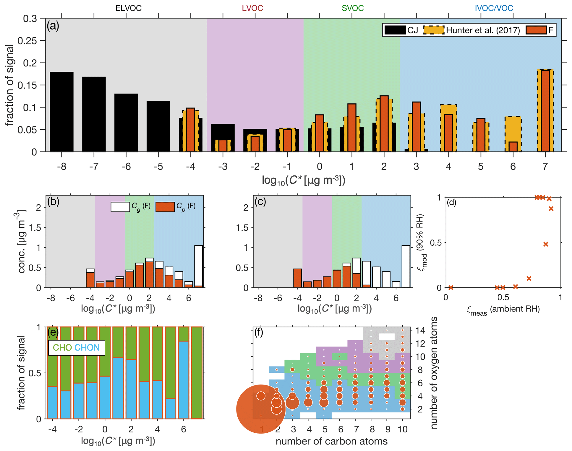
Figure 2 (a) The normalized volatility distributions (C_g+C_p) from Cappa and Jimenez (2010; CJ) and the BAECC FIGAERO–I-CIMS measurements (F) using the modified Li et al. (2016) molecular-formulae-based parameterizations. A volatility distribution from Hunter et al. (2017) constructed from the BEACHON-RoMBAS measurement campaign is shown by the dashed bars. The volatility ranges for ELVOC, LVOC, SVOC, and IVOC/VOC are shown in color scales. These C^∗ limits apply throughout the paper. (b–c) The partitioning predicted based on the FIGAERO–I-CIMS gas- and particle-phase measurements and the PARSEC–UFO, respectively. The PARSEC–UFO partitioning corresponds to 90 % RH, while the ambient observation is under ambient RH. (d) A scatterplot drawn between the FIGAERO–I-CIMS-derived partitioning coefficients (ξ_meas) and PARSEC–UFO-derived coefficients (ξ_mod) for the 12 different volatility bins. Panels (e)–(f) represent the gas-phase molecular composition from the FIGAERO–I-CIMS. Panel (e) shows the distribution between organic nitrates and non-nitrates, and panel (f) shows the degree of oxygenation in the form of oxygen and carbon numbers. The marker size in panel (f) corresponds to the concentration of signal for the given n_C and n_O combination.

2.3.2 Volatility distributions from FIGAERO–I-CIMS data (F distributions)

Organic aerosol volatility distributions from FIGAERO–I-CIMS measurements conducted during BAECC (Mohr et al., 2017, 2019; Schobesberger et al., 2016; Lee et al., 2018, 2020) are also derived. It can be assumed that the FIGAERO–I-CIMS detected most of the OA measured with the ACSM because FIGAERO–I-CIMS is sensitive to oxidized organic species, such as organic acids (Lutz et al., 2019), and most of the observed OA mass (∼ 95 %) measured by the ACSM can be attributed to oxygenated organic aerosol, which is thought to represent organic acids (Yatavelli et al., 2015). The agreement between the two measurements is supported by the comparison between the daytime FIGAERO–I-CIMS particle-phase signal (of identified ions) and the OA mass concentration retrieved from ACSM measurements (provided in Fig. S3). While the quantification of the FIGAERO–I-CIMS measurements remains challenging, and therefore while a quantitative comparison between the concentrations is uncertain, the high correlation between measurement data (Pearson R= 0.79) proves that the instruments generally sample the same aerosol population. Notably, the PARSEC–UFO simulations use OA mass fraction (f_Org) only from the ACSM measurements. The volatility distributions are derived from FIGAERO–I-CIMS data using molecular formula parameterizations derived under 300 K in Li et al. (2016):

$$\begin{array}{}\text{(18)}& \begin{array}{rl}{\log }_{\mathrm{10}}{C}^{\ast }\left(T_{\mathrm{ref}}\right)& =\left(n_{\mathrm{C}}^{\mathrm{0}}-n_{\mathrm{C}}\right)b_{\mathrm{C}}-n_{\mathrm{O}}{b}_{\mathrm{O}}\\ & -\mathrm{2}{\displaystyle \frac{n_{\mathrm{C}}{n}_{\mathrm{O}}}{\left(n_{\mathrm{C}}+n_{\mathrm{O}}\right)}}{b}_{\mathrm{CO}}-n_{\mathrm{N}}{b}_{\mathrm{N}},\end{array}\end{array}$$

where $n_{\mathrm{C}}^{\mathrm{0}}$ is a reference carbon number; b_C, b_O, and b_N are the contributions of each carbon, oxygen, and nitrogen atom to the log ₁₀C^∗, respectively; b_CO is a so-called carbon-oxygen non-ideality parameter (Donahue et al., 2011); and n_C, n_O, and n_N are the numbers of carbon, oxygen, and nitrogen atoms in the molecular formulae assigned for the FIGAERO–I-CIMS data during high-resolution peak fitting of the measured mass spectra. The b values utilized are listed in Li et al. (2016). In their recent work, Huang et al. (2021) derived volatility distributions from various organic vapor measurements from SMEAR II. They adjusted the Li et al. (2016) parameterization for organic nitrates. As shown in Isaacman-VanWertz and Aumont (2021), the utilization of the Li et al. (2016) parameterization for OA rich in organic nitrates leads to biased vapor pressure estimates. Organic nitrates are known to form in the boreal air as a result of nitrate radical chemistry, which is pronounced during the night, along with daytime oxidation of monoterpenes in the presence of nitric oxide (e.g., Yan et al., 2016; Zhang et al., 2020). To account for these nitrates, Huang et al. (2021) followed the suggestions presented in Daumit et al. (2013) and treated all the nitrate functional groups as hydroxyl (−OH) groups. Given that the focus of this study is on the same measurement site as Huang et al. (2021), their methodology for deriving a volatility distribution from the FIGAERO–I-CIMS is followed here. Once the volatility distributions are constructed using Eq. (18) for 300 K (reference temperature), their adjustments to the parcel model simulation initial temperatures using Eq. (13) is performed.

The volatilities are calculated for the 1596 ions identified by the FIGAERO–I-CIMS measurements. Afterwards the signals are binned with a decadal spacing so that all the ELVOC and LVOC are summed into one bin at $C^{\ast }={\mathrm{10}}^{-\mathrm{4}}$ µg m⁻³. The highest volatilities reached $C^{\ast }={\mathrm{10}}^{\mathrm{7}}$ µg m⁻³, which is therefore set as the upper limit of the volatility distribution. Following from this, the volatility span is ${\log }_{\mathrm{10}}{C}^{\ast }=[-\mathrm{4},\mathrm{7}]$. The campaign average volatility distribution is shown in red bars in Fig. 2a. The average CJ distribution exhibits generally higher fractions in the ELVOC region compared to the F distribution (Fig. 2a). This mostly results from the low/non-existent SVOC and IVOC concentrations in the CJ distribution. As the ELVOCs and LVOCs contain little or no gas-phase signals post-initialization, the F distribution used as input for PARSEC–UFO simulations uses the volatility span of ${\log }_{\mathrm{10}}{C}^{\ast }=[\mathrm{0},\mathrm{7}]$ to speed up the simulations.

The average F distribution shows a remarkable agreement with the organic volatility distributions from the BEACHON-RoMBAS field campaign conducted at the Manitou Experimental Forest Observatory in the Colorado Rocky Mountains in summer 2011 (Hunter et al., 2017; see Fig. 2a). Initially, Hunter et al. (2017) derived a volatility distribution for the total atmospheric reactive carbon (other than CH₄, CO₂, and CO) using six different types of measurements and assuming minimal overlap among the measured species. Here, the Hunter et al. (2017) distribution is displayed in Fig. 2a after shifting it to the mean PARSEC–UFO initialization temperature (280 K) using Eq. (13) and subtracting non-oxygenated VOC signals from it for comparison. The Hunter et al. (2017) distribution is not used in PARSEC–UFO simulations; it is only shown for comparative purposes due to its similarity with the F distributions.

In Fig. 2b and c, the partitioning coefficients ξ_q from the PARSEC–UFO initialization (see Sect. 2.2) are compared against the partitioning suggested by the FIGAERO–I-CIMS measurements, where the C^∗ correspond to the mean PARSEC–UFO initialization temperature and range from ${\log }_{\mathrm{10}}{C}^{\ast }=[-\mathrm{4},\mathrm{7}]$. The concentrations in volatility bins with ${\log }_{\mathrm{10}}{C}^{\ast }\le$ 1 agree, suggesting that the majority of the organics in these bins are in the particle phase. Similarly, the agreement in the highest-volatility bin (${\log }_{\mathrm{10}}{C}^{\ast }=$ 7) suggests the presence of gas-phase compounds only in both distributions. The estimations of the gas phase vary between ${\log }_{\mathrm{10}}{C}^{\ast }=[\mathrm{1},\mathrm{7}]$, showing a higher gas-phase fraction for the modeled partitioning coefficients (Fig. 2b–d). This variability can result from numerous reasons which, apart from uncertainties related to measurements and parameterizations, include viscous particle coatings inhibiting equilibration between gas and particle phases and therefore show high particle-phase concentrations of high-volatility compounds in the observations. Alternatively, these concentrations can also result from the thermal decomposition of lower-volatility products during the FIGAERO–I-CIMS heating process (Lopez-Hilfiker et al., 2015) or from the tendency of the Eq. (18) parameterization to underestimate the volatility of organic nitrates (Graham et al., 2023; despite treating the −NO₃ groups as −OH groups) shown to be abundant in the BAECC FIGAERO–I-CIMS data set (Fig. 2e). Understanding these differences is important and requires further analysis.

The molecular composition of the gas-phase compounds detected by the I-CIMS during BAECC is analyzed and presented in detail in Lee et al. (2018). In the following, the average composition of each volatility bin during daytime is briefly described. Except for the highest-volatility bin, nitrogen-containing species (CHON), which are prominently organic nitrates at SMEAR II (Huang et al., 2021), make up significant mass fractions of each bin in the gas phase (Fig. 2e). Figure 2f shows the concentration of the gas-phase compounds as a function of the compound carbon and oxygen atom numbers. The figure shows how ELVOCs and LVOCs have the highest numbers of both carbon and oxygen atoms. IVOCs and SVOCs comprise compounds with highly variable carbon skeleton lengths, but the number of oxygen atoms per compound remains low and is notably always lowest for IVOCs and VOCs. Formic acid (HCOOH) makes up most of the gas-phase signal. It is distributed in the most volatile volatility bin ($C^{\ast }={\mathrm{10}}^{\mathrm{7}}$ µg m⁻³). HCOOH is one of the most abundant carboxylic acids in the atmosphere and rainwater (e.g., Galloway et al., 1982; Millet et al., 2015, and references therein) and is known to have various sources and precursors (Millet et al., 2015). The I-CIMS measurements discussed here were also performed as part of an eddy covariance flux measurement setup during BAECC (Schobesberger et al., 2016). These flux measurements provided insight into the high HCOOH concentrations possibly due to high emissions from the boreal forest ecosystem. More details from these results can be found in Schobesberger et al. (2016).

2.4 UK Earth System Model (UKESM1) simulations

To evaluate the frequency of times size distributions yielding high ΔCDNC (which is the percent change in CDNC due to co-condensation) during BAECC would become evident over the boreal biome in an Earth system model (ESM) if a parameterization of co-condensation were implemented, the United Kingdom Earth System Model (UKESM1, Sellar et al., 2019; Mulcahy et al., 2020) is utilized. The simulations performed with UKESM1 are configured for Atmospheric Model Intercomparison Project (AMIP)-style simulations, where UKESM1 is run in its atmosphere-only configuration with time-evolving sea surface temperature and sea ice, as well as prescribed marine biogenic emissions from fully coupled model simulations. In addition to the HadGEM3-GC3.1 core physical dynamical model of the atmosphere, land, ocean, and sea ice systems (Ridley et al., 2018; Storkey et al., 2018; Walters et al., 2017), UKESM1 also contains additional component models for atmospheric chemistry and ocean and terrestrial biogeochemistry for carbon and nitrogen cycle representation. The version of UKESM1 used includes developments to the droplet activation scheme from Mulcahy et al. (2020) to facilitate more consistent comparisons against PARSEC–UFO. In the standard configuration of UKESM1, aerosol particles are activated into cloud droplets using the droplet activation parameterization of Abdul-Razzak and Ghan (2000). An alternative optional configuration of UKESM1 was employed that uses the Barahona et al. (2010) droplet activation parameterization, which has been shown to be more consistent when compared against an adiabatic cloud parcel model over a range of conditions (Simpson et al., 2014; Partridge et al., 2015). Furthermore, in the standard configuration of UKESM1, the droplet activation scheme uses the distribution of sub-grid variability in the updraft velocities, according to West et al. (2014), with updates as described in Mulcahy et al. (2018). To facilitate more consistent comparisons against PARSEC–UFO simulations that calculate droplet number using a single average updraft velocity, the single characteristic updraft velocity (Peng et al., 2005) was used to initialize the droplet activation scheme in UKESM1.

A N96L85 horizontal resolution structure (1.875° × 1.25° longitude–latitude, which corresponds roughly a horizontal resolution of 135 km) is chosen for the simulations, and the vertical space is split to 85 levels (50 levels between 0 and 18 km and 35 levels between 18 and 85 km). In this study, the model is run in a nudged configuration (horizontal wind nudging (but not temperature) between model levels 12 and 80, with a constant 6 h relaxation time) for the years 2009–2013 inclusively. External forcing and emission data sets are consistent with the Coupled Model Intercomparison Project Phase 6 (CMIP6) implementation as described in Sellar et al. (2020). The simulation setup is same as in the Aerosol Comparisons between Observations and Models (AeroCom) Phase III GCM (global circulation model) Trajectory experiment (AeroCom, 2022; Kim et al., 2020).

The UKESM1 aerosol scheme represents the particle size distributions with the following five log-normal modes: the nucleation soluble mode, Aitken soluble and insoluble modes, accumulation soluble mode, and coarse soluble mode (Mulcahy et al., 2020). The aerosol microphysical processes of new particle formation (NPF), condensation, coagulation, wet scavenging, dry deposition, and cloud processing are handled with GLOMAP (Global Model of Aerosol Processes; Mann et al., 2010; Mulcahy et al., 2020). The UKESM1 NPF mechanism follows the parameterization derived in Vehkamäki et al. (2002) for binary homogeneous nucleation of H₂SO₄ and water. A separate boundary layer NPF is not included in the simulations (Mulcahy et al., 2020). The soluble aerosol size distribution log-normal aerosol modal parameters (nucleation mode, soluble Aitken mode, and soluble accumulation mode) and sub-grid-scale updraft velocities with a 3 h time resolution at the cloud base of stratiform clouds are used. These diagnostics are subsequently masked to include only data in which activated aerosol particles exceeds zero and the temperature exceeds 237.15 K, in keeping with criteria used by the droplet activation scheme. The PNSD modal parameters are used to construct aerosol size distributions. In UKESM1 the geometric standard deviations are fixed parameters. The same values are used for consistency for the modes that are accounted for in this work. The geometric standard deviation for UKESM1 nucleation soluble mode and the Aitken soluble mode is 1.59, and for the accumulation soluble mode it is 1.40. UKESM1 outputs for the Aitken insoluble mode and soluble coarse mode are not used in analysis performed in this study. UKESM1 uses a 26 % SOA yield from monoterpenes, the emissions of which are from the Model of Emissions of Gases and Aerosols from Nature (MEGAN) version 2.1 (Guenther et al., 1995).

3 Results and discussion

3.1 Organic condensation: time and volatility dependencies

The first PARSEC–UFO simulation results (Fig. 3) correspond to initializing the model with data collected on 11 May 2014 at 13:37 EET (eastern European winter time). This simulation is identified from the full data set as one that represents a median cloud response to co-condensation of organics and water. Figure 3a shows the vertical evolution of total SVOC and IVOC concentrations in the gas phase for the three different updraft scenarios (w= 0.1, 0.3, or 1 m s⁻¹, respectively). Both SVOC and IVOC concentrations decrease significantly along the adiabatic ascent in sub-saturated conditions below cloud base (CB). Given that the PARSEC–UFO simulation output is saved with 2 m vertical resolution, “below CB” contains all the simulation output under sub-saturated conditions, and the RH at CB is defined as $min(\text{RH}\ge$ 100 %). When moving to saturated conditions, SVOCs and IVOCs are scavenged. This result is in line with Bardakov et al. (2020), who modeled complete gas removal of volatility bins up to roughly ${\log }_{\mathrm{10}}{C}^{\ast }=$ 9 within convective clouds.

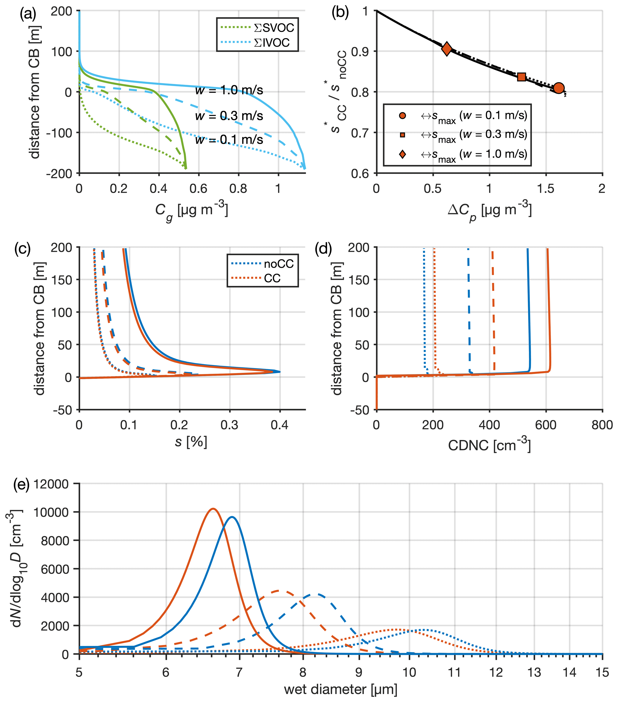
Figure 3 A summary of simulated cloud microphysics on 11 May at 13:37 EET during the BAECC campaign. Simulations are performed both with and without organic condensation (red and blue lines, respectively) for three different updraft velocities (see line styles in panel a). The initial temperature is 279 K, pressure 980 hPa, and RH is 90 %. (a) The concentration of SVOCs and IVOCs in the gas phase as a function of distance from cloud base (CB). SVOCs have ${\log }_{\mathrm{10}}{C}^{*}=[\mathrm{0},\mathrm{2}]$ and IVOCs ${\log }_{\mathrm{10}}{C}^{*}=[\mathrm{3},\mathrm{7}]$ under 279 K. (b) The relative change in critical supersaturation (s^∗) between noCC and CC simulations, as a function of soluble mass added along the ascent by condensing organics in the simulations, where co-condensation is enabled. The data are shown for a particle with a dry diameter of 147 nm at PARSEC–UFO initialization. The markers represent the reductions at the time when maximum supersaturation (s_max) was reached. (c–d) The evolution of the s_max and CDNC with altitude, respectively. (e) The droplet spectra 50 m above CB. Size bins exceeding the critical diameter as predicted by Köhler theory are calculated as cloud droplets. The red lines are obtained with F volatility distributions (Fig. 2a). The line type specifications in panels (d)–(e) follow those shown in panel (a), and the colors used in panels (d)–(e) are documented in the panel (c) legend.

When considering all 97 simulations, the net mass fractions of organics condensed below CB are on average 91 %, 70 %, and 28 % for the 0.1, 0.3, and 1.0 m s⁻¹ updraft, respectively, which in absolute concentrations means additions of 1.8, 1.4, and 0.7 µg m⁻³ to the aerosol particle soluble mass (Table 2). The yielded mass concentrations are in the same order of magnitude as the PM₁ mass concentrations measured during BAECC (interquartile range, IQR: 0.95, 1.95, and 3.22 µg m⁻³ from ACSM data), which means that such organic condensation along the adiabatic ascents as simulated here would yield roughly a doubling of the soluble mass due to SVOC and IVOC condensation below CB. Figure 4d–f show the simulated organic condensate concentrations for each volatility bin. While the condensed fraction for the highest-volatility bin is smallest (Fig. 4a–c), the absolute concentrations of condensate are amongst the largest due to the high availability of organic vapor in the highest-volatility bin (mostly HCOOH; Sect. 2.3.2). The condensation efficiency of the highest-volatility bin correlates with the number of large particles serving as condensation sink for vapors (Fig. S4). This suggests that these organic vapors are likely to condense onto larger particles, which are susceptible to be activated into cloud droplets regardless of co-condensation. Similar correlations are observed to a lesser extent with the ${\log }_{\mathrm{10}}{C}^{\ast }=$ 6 volatility bin (not shown). In this work, the information of the size ranges of particles which the high-volatility IVOCs condense onto is lacking. Therefore, more systematic studies should be conducted to better understand whether the condensation of the high-volatility IVOCs onto ultrafine particles is sufficient enough to lead to increased droplet activation.

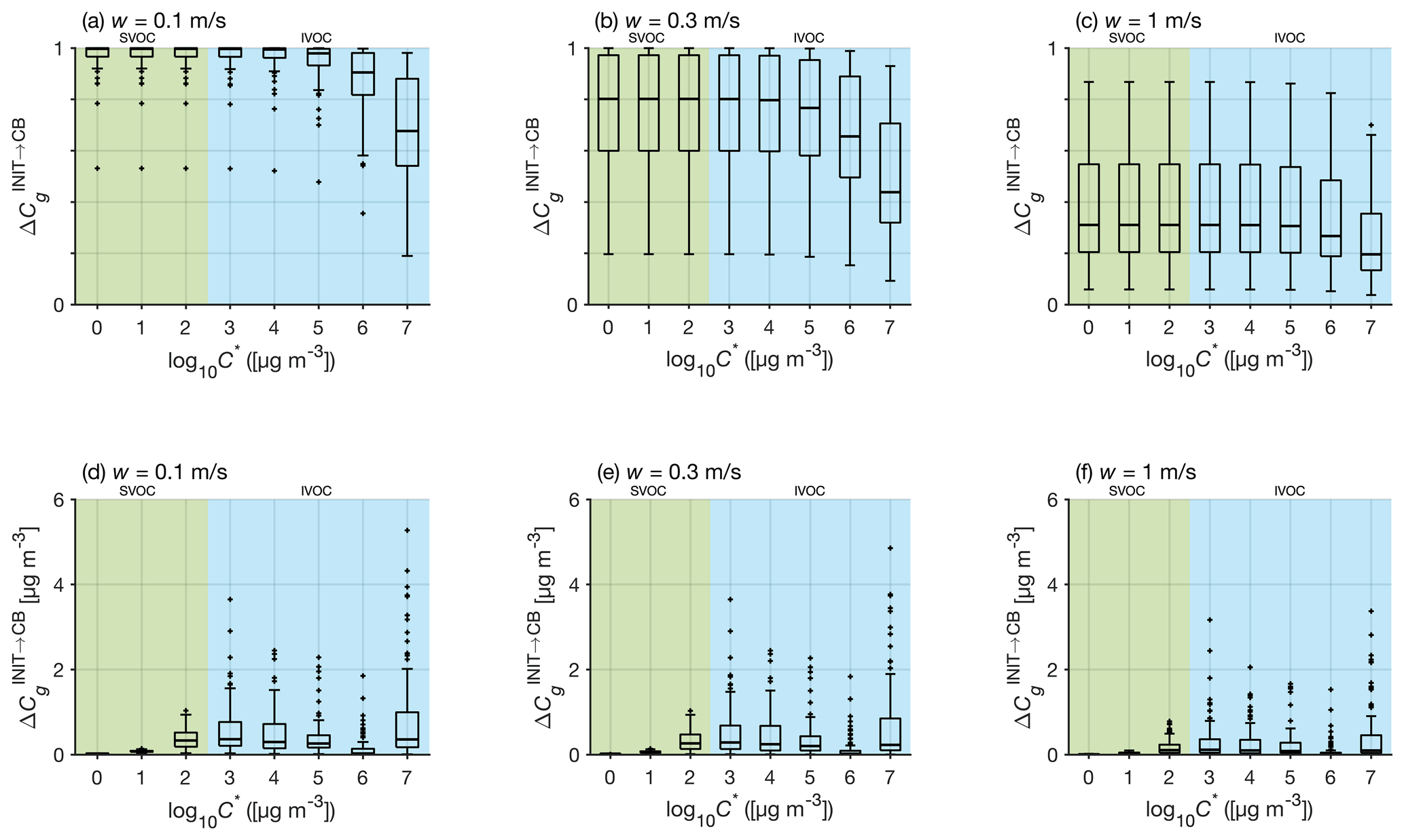
Figure 4 Box plots showing the fractions (a–c) and absolute concentrations (d–f) of organic vapor condensed below cloud base per volatility bin for the 0.1, 0.3, and 1.0 m s⁻¹ updraft scenarios, respectively. The shaded backgrounds reflect SVOC (green) and IVOC/VOC (blue) volatility ranges under the PARSEC–UFO initialization temperature.

The exact numbers presented here should, however, be assessed with caution, as an ideal liquid phase and the partitioning being determined by mole fractions of water-soluble organics are assumed (Sect. 2.1.1). Topping et al. (2013) looked into the assumption of ideality in their Supplement. They found it to enhance the amount of modeled organic condensate compared to a non-ideal case. However, their simulations exploring non-ideality with organic activity coefficients predicted with the UNIFAC method (UNIQUAC Functional-group Activity Coefficients; Fredenslund et al., 1975) still led to significant amounts of condensed organic mass. The impact of the ideality assumption was shown to be most significant in their highest-volatility bin ($C^{\ast }=$ 1000 µg m⁻³). Activity coefficients (and solubilities) of organics should be better constrained in the future to assess the impact on volatility bins of ${\log }_{\mathrm{10}}{C}^{\ast }>$ 3, which was not explored in Topping et al. (2013). As discussed in the Topping et al. (2013) Supplement, it is likely that solubility decreases towards the higher-volatility bins. Here, a simple assessment of the assumption of ideality (Appendix A; Fig. A2b) suggests that the gained organic soluble mass reduces only when the overall mass accommodation coefficient for organics is less than 0.4. This would mean that the organic condensation shown here could be taken as the upper limit.

Further investigation on how efficiently different volatility bins condensed along the adiabatic ascents across all the 97 simulation scenarios repeated with the three fixed updraft velocities is also performed (Fig. 4a–c). In the 0.1 m s⁻¹ updraft scenario, almost all organic vapor condenses up to ${\log }_{\mathrm{10}}{C}^{\ast }=$ 5, and the condensation capability of the highest-volatility bin (${\log }_{\mathrm{10}}{C}^{\ast }=$ 7) shows the highest variability (∼ 20 %–91 % condensed below CB; Fig. 4a). The same features can be observed with the 0.3 and 1.0 m s⁻¹ updraft simulations, although the fraction of organic vapor condensed per volatility bin is reduced (in the w= 1 m s⁻¹ scenarios only ca. 30 % of the vapor condenses below CB; Fig. 4b–c). The results from these simulations reveal that there is only enough time under slow adiabatic ascents for most of the organic vapor to condense.

3.2 Impact of meteorological conditions on the sensitivity of cloud microphysics to organic vapor condensation

As explained previously in Topping et al. (2013), the CDNC enhancements associated with co-condensation arise from the increase in organic solute concentration, which decreases the critical supersaturation (s^∗) needed for a given particle to activate. The s^∗ is reduced about 10 %–20 % for the case on 11 May 2014 at 13:37 EET presented in Fig. 3b when co-condensation is enabled. This reduction is calculated for a particle with a dry radius of 71.9 nm (i.e., the smallest activated dry radius when co-condensation is disabled, $r_{\mathrm{noCC}}^{\ast }$). Figure S5 shows the development of the wet particle size as a function of altitude in the PARSEC–UFO simulation summarized in Fig. 3. It clearly demonstrates the differences introduced by co-condensation through the activation of new size bins (four size bins in total when w= 0.1 m s⁻¹) that would have remained as interstitial aerosol particles in the simulations where co-condensation is turned off. The enhanced growth of more particles due to co-condensation enhances the water vapor condensation sink, which leads to a reduction in the achieved maximum ambient supersaturations (s_max; see Fig. 3c for the 11 May case and Table 2 summarizing all 97 simulations). As the meteorological conditions are the same in simulations performed with and without co-condensation, the condensation sink dictates the changes in s_max (Eq. 3). A reduced s_max would typically lower the number of aerosol particles activating into cloud droplets, but here the reductions in s^∗ are greater than the reductions in s_max, which therefore lead to an enhanced CDNC (see Fig. 3b–c for the 11 May case). This can be interpreted as a competition effect between the s_max and s^∗ reductions, respectively, which the s^∗ reduction wins. When examining the 0.1 m s⁻¹ updraft case in the 11 May simulation shown in Fig. 3, the s_max is reduced ∼ 7 %, which is less significant than the s^∗ reduction of ∼ 20 %. This leads to a 22 % enhancement in CDNC (Fig. 3d), as r^∗ reduces from 72 to 66 nm ($\mathrm{\Delta }{r}^{\ast }\approx$ 6 nm). Figure 3e shows the droplet spectrum for the 11 May case, which highlights the consistent shift in droplet sizes to smaller diameters due to organic co-condensation (see also Fig. S5, which displays the same 11 May simulation with w= 0.1 m s⁻¹). The impact such a shift could have on cloud lifetime and precipitation should be studied further.

The modeled BAECC campaign median CDNC values (over the 97 simulations) without co-condensation are on average 161, 300, and 530 cm⁻³ in modeling scenarios utilizing 0.1, 0.3, and 1.0 m s⁻¹ updrafts, respectively (Table 2). CDNC is shown to correlate well with the accumulation mode number concentration (N₂) and at times with the Aitken mode number concentration (N₁) if the Aitken mode particles are large enough in size and accompanied with strong enough updrafts and a low N₂ (Fig. S6). The reductions in the smallest activated dry radii due to co-condensation ($r_{\mathrm{noCC}}^{\ast }-r_{\mathrm{CC}}^{\ast }$) are on average ∼ 8, ∼ 7, and ∼ 5 nm for the modeling scenarios utilizing 0.1, 0.3, and 1.0 m s⁻¹ updrafts, respectively, and the corresponding median ΔCDNC values are ∼ 16, ∼ 23, and ∼ 19 %, respectively (Table 2 and Fig. 5a). The swarm plot in Fig. 5a shows that ΔCDNC and CDNC do not correlate; i.e., low CDNC in the noCC runs does not favor high ΔCDNC.

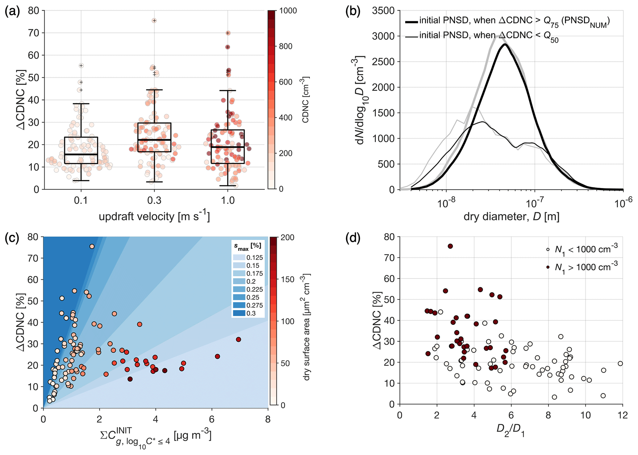
Figure 5 (a) Box plots showing the predicted ΔCDNC (using F volatility distributions) due to co-condensation in the three different modeling scenarios (0.1, 0.3, and 1.0 m s⁻¹ updrafts). The colorful markers represent CDNC (without accounting for co-condensation) in form of a swarm plot. The median (Q₅₀) ΔCDNC values yielded using the CJ distribution are shown in Fig. S7. (b) The median initial dry size distributions calculated from the simulations exceeding the 75th percentile in ΔCDNC (>Q₇₅; thick lines) and remaining below the ΔCDNC median (<Q₅₀; thin lines), respectively. The PNSD medians are calculated by taking a median of the PNSD calculated using the log-normal parameters from both sets of simulations (in black) and from the measurement data (in gray). The data are shown for the simulation performed with a 0.3 m s⁻¹ updraft. (c) The relationship between the modeled ΔCDNC and the initial organic vapor concentration within the log ₁₀C^∗ ranges from −4 to 4 ($C_{\mathrm{g},-\mathrm{4}:\mathrm{4}}^{\mathrm{INIT}}$). The marker color-coding represents the initial dry size distribution surface area (S). The plot background is colored with the modeled maximum supersaturations (s_max). These are calculated from s_max binned ΔCDNC vs. $C_{\mathrm{g},-\mathrm{4}:\mathrm{4}}^{\mathrm{INIT}}$ linear fit 90 % confidence intervals (CI; area between CI is colored). The figure shows that S anticorrelates with s_max (see Eq. 3). The data are shown for the simulations performed with a 0.3 m s⁻¹ updraft only. (d) The figure evaluates how well the simple criteria ($D_{\mathrm{2}}/D_{\mathrm{1}}<$ 6 and N₁> 1000 cm⁻³) works on the PARSEC–UFO simulations.

On average during the BAECC simulation period (97 simulations), the highest ΔCDNC are found when initializing the model with a 0.3 m s⁻¹ updraft velocity (also visible in Fig. 3d for the 11 May case), followed by ΔCDNC predictions for the 1 m s⁻¹ case. In the latter case, high supersaturations are achieved, leading to the formation of many cloud droplets, yet the effects of co-condensation remained less pronounced as the high ascent speed poses kinetic limitations for organic condensation (see Sect. 3.1 and Fig. 4). Despite the highest organic uptake in the 0.1 m s⁻¹ updraft simulations (Fig. 4a, d), the ΔCDNC value remains the lowest. This can be explained by the low s_max, which remains insufficient to activate small particles to cloud droplets ($r_{\mathrm{noCC}}^{\ast }\sim$ 64 nm; Table 2). As the Aitken mode possesses most particles in terms of number (Table 1), the few nanometer reductions in r^∗ affect ΔCDNC the most when the r^∗ reduction takes place on the steep PNSD slopes (strongly negative $\mathrm{d}/\mathrm{d}{\log }_{\mathrm{10}}D$ ($\mathrm{d}N/\mathrm{d}{\log }_{\mathrm{10}}D)$) between the Aitken and accumulation mode. When the updraft velocity is low (0.1 m s⁻¹), the r^∗ are too large to overlap with the parts of the PNSD with a high slope, even if r^∗ reduces greatly due to co-condensation. Due to the high-updraft dependency of the modeled ΔCDNC, future process modeling work should consider performing simulations following updraft probability density functions (PDFs), as used in some GCMs, and calculating PDF-weighted CDNC values (West et al., 2014). In this way, more weight will be given to lower updrafts, and the model outputs will be more robust since in reality the sub-grid scale updraft velocity at cloud base is highly variable.

Besides updraft velocity, the modeled ΔCDNC are also affected by PARSEC–UFO initialization temperatures. This can be seen when the effect of the volatility distribution upgrade (from CJ to F) on the modeled ΔCDNC is investigated. For this purpose, an additional set of PARSEC–UFO simulations using the CJ volatility distribution is performed. The CDNC enhancements due to co-condensation attained with the CJ volatility distribution are negligible (median ΔCDNC is 0; Fig. S7) and therefore strikingly different from those presented in Topping et al. (2013). The large difference in the modeled ΔCDNC between the F and CJ simulations arises from the low amount of organic vapor available for condensation ($\sum C_{\mathrm{g}}^{\mathrm{INIT}}$ is only 0.10 µg m⁻³ in CJ simulations, while in the F simulations it is 2.05 µg m⁻³), which in turn results from the low PARSEC–UFO initialization temperature attained from the radio soundings (Sect. 2.3). If the initialization temperatures were higher, more organic vapor would remain in the gas phase after PARSEC–UFO initialization and a larger ΔCDNC could be modeled. The simulations performed in Topping et al. (2013) were initialized at 298 K, which explains why they report significant CDNC enhancements due to co-condensation using a similar CJ volatility distribution to the one used here. We can reproduce the Topping et al. (2013) findings when increasing the initialization temperature with PARSEC–UFO (see Fig. S8) and also demonstrate that by decreasing the initialization temperature from 298 to 280 K (the BAECC median temperature), the ΔCDNC modeled by Topping et al. (2013) should also be negligible (Fig. S8). These findings emphasize the critical role of the initialization temperature (and assumptions made on equilibrium upon model initialization) as this impacts the amount of organic vapor present in the gas phase prior to the air parcel's ascent.

Additionally, the result suggests high importance of organic vapors with saturation vapor concentrations exceeding ${\log }_{\mathrm{10}}{C}^{*}=$ 3 (under 298 K) for co-condensation. If one were to utilize CJ distributions in future co-condensation work, one could consider multiplying the highest-volatility bins, e.g., with a carefully selected constant. Similar approaches have been used previously when modeling SOA formation from IVOCs (Lu et al., 2020).

As the results from Fig. 4 underline the time-dependence of co-condensation (Sect. 3.1), it is worth remembering that the PARSEC–UFO initialization RH is set to 90 % where equilibrium conditions are assumed (see Sect. 2.4 and 2.2). Therefore, the kinetic effects play a role only from 90 % to 100 % RH. Importantly, if the initial RH was set to a lower value, more time would be available for co-condensation before reaching CB, and if the initial RH was set to a higher value, less time would be available. On the other hand, due to the assumption of initial equilibrium conditions, a lower initial RH also ensures a higher organic vapor concentration available for co-condensation, and a higher initial RH reduces the organic vapor availability. Together with initial temperature, the initial RH strongly controls the amount of organic vapor available for co-condensation (Appendix A; Figs. A1 and S3) and thereby the amount of soluble organic mass yielded by the time the air parcel reaches cloud base. While the decision to maintain a fixed initial RH for the different simulations has proven useful for this study as it eases the data interpretation process, it should be acknowledged that the initial RH could be better constrained in future simulations. Naturally, the organic vapor condensation depends on the initial RH, and as a result ΔCDNC is also sensitive to the selection of the initial RH (Fig. A1). If the initial RH is set to 60 %, CDNC enhancements as high as ∼ 100 % could be expected, while if the initial RH is set to 99 %, the enhancements are expected to range between 0 and ∼ 20 %. This variation is greater than the impact the ideality assumption (or the selection of vaporization enthalpy) has on ΔCDNC (Sect. 3.1; Appendix A).

3.3 Impact of initial aerosol size distribution and organic vapor concentration on the sensitivity of CDNC to organic vapor condensation

As briefly mentioned in the previous section, PNSD affects ΔCDNC along with the initial meteorological conditions. The importance of Aitken mode in ΔCDNC associated with turning co-condensation on in PARSEC–UFO is exemplified in Fig. 5b for the 0.3 m s⁻¹ updraft simulations. In this figure, the initial dry PNSD are averaged from the simulations with the highest 25 % and lowest 50 % modeled ΔCDNC, respectively. The PNSD corresponding to the highest 25 % of the modeled ΔCDNC has a very minor accumulation mode and a large Aitken mode (with respect to the mode total number concentrations; i.e., N₂ and N₁, respectively) with a diameter (D₁) of ∼ 40 nm (D₂ is ∼ 110 nm). It is named PNSD_NUM, where NUM refers to a strong nascent ultrafine mode characteristic of the shown size distribution. The PNSD_NUM values gain the highest ΔCDNC despite a relatively small change in the smallest activated dry radii because of the steep PNSD slope in the size range where the smallest activated dry radii reduce (Fig. S9). The slope compensates for a comparatively small reduction in the smallest activated dry radii by sharply increasing the number of particles that activate when co-condensation is enabled. The PNSD corresponding to the lowest 50 % of the modeled ΔCDNC is strongly bimodal, where the Aitken and accumulation modes are almost equal in terms of N. Moreover, the two modes are separated by a clear Hoppel minimum (Hoppel and Frick, 1990). The Hoppel minimum is characteristic for aerosol populations which have undergone cloud processing. The PNSD associated with the lowest ΔCDNC values tend to have the smallest activated dry radii close to the Hoppel minimum, which is where the PNSD slope is negligible (Fig. S10). Therefore, the integral through this range provides fewer particles to be activated to cloud droplets, and the ΔCDNC values remain low. It should be noted, however, that the reductions in the smallest activated dry radii are on average higher in the simulations initialized with PNSD_NUM (Fig. S11a) due to higher availability of organic vapors (Fig. S11b) and their condensation to a more critical size range. Nonetheless, it is evident that the shape of the PNSD dictates the magnitude of the ΔCDNC, as a ∼ 4 nm reduction in the smallest activated dry radius can lead to a CDNC enhancement of ∼ 45 % in the case of a PNSD_NUM, while in the case of a PNSD with a Hoppel minimum, ΔCDNC would be only ∼ 10 % (Fig. S11). These results underline that environments rich in particles from a local source would be more susceptible to high ΔCDNC due to co-condensation, while regions with aged and cloud-processed size distributions are affected less (here ΔCDNC < 20 %; Fig. 5a).

Interestingly, a PNSD_NUM was found to be important when looking into suitable conditions for large increase in CDNC caused by surface active organics (Ovadnevaite et al., 2017; Lowe et al., 2019). Lowe et al. (2019) utilized a similar CPM (ICPM; Sect. 2.1) to the one used in this study (notably without co-condensation) but enabled a fraction of the particulate organics to form a thin, max 0.2 nm thick, film around the particle. The film was characterized by a surface tension of 40 mN m⁻¹ as opposed to the surface tension of pure water (72.8 mN m⁻¹). The idea of this compressed film (CF) approach was to simulate the surface tension reductions caused by organic species leading to the activation of smaller particles to cloud droplets at the coastal Mace Head site (Ovadnevaite et al., 2017). Through sensitivity studies, Lowe et al. (2019) found that the largest percent change in CDNC due to surface active organics (> 10 %) took place in Mace Head when $N_{\mathrm{2}}<a{N}_{\mathrm{1}}^b+c$ (a= 602, b= 0.0884, and c= −766). The increase in CDNC in the Lowe et al. (2019) study was also attributed to the reduction in s^∗ when comparing against simulations where the surface tension was that of water. Moreover, the same competition effect between s_max and s^∗ reductions – as described in Sect. 3.2 – was demonstrated in their study but just triggered by different chemical parameters. The sensitivity of the CDNC enhancements to PNSD_NUM in this study, as well as in Lowe et al. (2019), demonstrates that the activation of fresh and non-cloud-processed aerosol particles is susceptible to small reductions in s^∗ that can be triggered, e.g., by organic surfactants or co-condensation. Importantly, potential surface activity also affects the CCN activation behavior of atmospheric organics (Ruehl et al., 2012, 2016; Lowe et al., 2019), correlating with volatility and solubility. The combined effect of all these three properties needs to be thoroughly investigated in the future.

In conjunction with the ΔCDNC susceptibility to PNSD_NUM, this study most critically highlights the importance of incorporating multimodal and representative size distributions in process modeling studies examining the cloud response to co-condensation (or surface-active organics, as demonstrated in Lowe et al., 2019). Topping et al. (2013), for example, used monomodal distributions (with varying log-normal parameters) in their study which could lead to overestimation of ΔCDNC, as size distributions with Hoppel minima are not explored. Multimodal distributions were used later by Crooks et al. (2018), but further explanation of the cloud response to increasing the number of modes remained lacking. In summary, our results together with the Lowe et al. (2019) results suggest that in clean environments with a local source of ultrafine particles, such as the boreal forest or marine environments, organic species in the presence of a NUM-featured PNSD can have significant impact on cloud properties either via co-condensation or through surface tension reductions.

Subsequently, a dry PNSD-based criterion for identifying regimes (conditions) in which co-condensation has the highest impact on CDNC is defined. It is found that restricting the ratio between the accumulation and Aitken mode geometric mean diameters in the initial dry PNSD to below 6 (i.e., $D_{\mathrm{2}}/D_{\mathrm{1}}<$ 6) and the Aitken mode number concentration to exceed 1000 cm⁻³ (i.e., N₁> 1000 cm⁻³) would yield ΔCDNC > 20 % in our simulations (Fig. 5d). Using the diameter ratio criterion, size distributions without a distinguishable Hoppel minimum are selected, which is characteristic in the simulations yielding the highest ΔCDNC (Fig. 5b), and the high N₁ ensures a high concentration of aerosol particles potentially activating into cloud droplets.

In addition to the PNSD_NUM features, the initial organic vapor concentration ($C_{\mathrm{g}}^{\mathrm{INIT}}$) also influences the modeled ΔCDNC. The extent to which the modeled ΔCDNC values are sensitive to $C_{\mathrm{g}}^{\mathrm{INIT}}$ is depicted in Fig. 5c, using the PARSEC–UFO simulations performed with 0.3 m s⁻¹ updrafts. The y axis represents the modeled ΔCDNC and the x axis the organic vapor concentration distributed in log ₁₀C^∗ bins within $[-\mathrm{4},\mathrm{4}]$ (denoted as $C_{\mathrm{g},-\mathrm{4}:\mathrm{4}}^{\mathrm{INIT}}$); i.e., in bins that do not show high dependency on the available surface area (see Sect. 3.2 and Fig. S4 for details). The relationship is not straightforward, but linear increases in ΔCDNC as a function of $C_{\mathrm{g},-\mathrm{4}:\mathrm{4}}^{\mathrm{INIT}}$ can be seen under constant, yet sufficiently high, s_max (here > 0.2 %). Under the modeled scenarios, where $s_{max}>$ 0.2 %, the $C_{\mathrm{g},-\mathrm{4}:\mathrm{4}}^{\mathrm{INIT}}$ is generally low (< 2 µg m⁻³). Still, the highest CDNC enhancements during the BAECC simulation period are achieved under these conditions. The high CDNC enhancements can be achieved – despite the low organic vapor abundance – simply because the soluble organic mass is distributed to more smaller particles. The markers in Fig. 5c are color-coded by the initial PNSD surface area, which under a constant updraft anticorrelates with s_max (see Eq. 3). ΔCDNC shows high sensitivity to $C_{\mathrm{g},-\mathrm{4}:\mathrm{4}}^{\mathrm{INIT}}$ when the dry PNSD surface area stays below a 100 µm² cm⁻³ threshold. Based on this analysis, it can be concluded that in the presence of a NUM-featured PNSD enabling the formation of high supersaturations (the dry PNSD surface area stays below 100 µm² cm⁻³), an adiabatic ascent with an updraft of 0.1 or 0.3 m s⁻¹ can yield ΔCDNC of > 40 % if 1 µg m⁻³ of co-condensable organic vapor is present in the rising air. This is a likely occurrence in the spring and summertime boreal forest (Huang et al., 2021). However, it should be noted that under such scenarios the modeled ΔCDNC values are highly sensitive to organic vapor concentration (Fig. 5c), and a reduction of ∼ 0.5 µg m⁻³ in organic vapor concentration can halve the modeled CDNC when the PNSD surface area is low. The simulations performed with the highest updraft velocity (w= 1.0 m s⁻¹) yield lower ΔCDNC under these clean conditions (ΔCDNC does not exceed 40 %), even though the simulated s_max values increase as opposed to the results obtained with lower updrafts (e.g., Table 2) because of the kinetic limitations hindering co-condensation (see Sect. 3.1).

3.4 Expected seasonality in the impact of co-condensation on CDNC at SMEAR II

In the following, the seasonality of the dry PNSD surface area at SMEAR II (6-year-long time series, 2012–2017) is investigated to estimate how often it stays below the previously mentioned threshold of 100 µm² cm⁻³; i.e., times when only 1 µg m⁻³ of co-condensable organic vapor present in the rising air could yield significant ΔCDNC. This is followed by an investigation of the frequency of the PNSD criteria ($D_{\mathrm{2}}/D_{\mathrm{1}}<$ 6 and N₁> 1000 cm⁻³) fulfillments in the long-term size distribution measurements at SMEAR II.

Figure 6a shows the seasonality of the dry surface area at SMEAR II. During daytime (09:00–19:00 EET), the surface area stays below the previously mentioned threshold 86 % of the time during the 2012–2017 measurement period (Fig. S12), which suggests that under 0.3 m s⁻¹ updraft velocities, generation of $s_{max}>$ 0.2 % at this site is likely. During summer months, the likelihood of surpassing the dry PNSD surface area threshold of 100 µm² cm⁻³ increases from 10 % to 22 % (Fig. S12) due to biogenic SOA formation (e.g., Tunved et al., 2006; Heikkinen et al., 2020), which grows the accumulation mode in the PNSD. Biogenic SOA formation depends on the SOA precursor, i.e., BVOC emissions and concentrations. Monoterpene concentrations are highest at SMEAR II in summer (Kontkanen et al., 2016; Hakola et al., 2012), as their emissions are strongly temperature-driven (Guenther et al., 1993). The organic vapor concentration available for co-condensation is therefore also highest in summer, but due to the enhanced surface area, the soluble organic mass is distributed to larger particles that dampen the cloud response to co-condensation. However, the monoterpene emission period is longer than just summer, and elevated monoterpene concentrations can be observed throughout the thermal growing season (when the daily average temperature is above 5 °C; Kontkanen et al., 2016; Hakola et al., 2012). Therefore, monoterpene emissions also take place at times when the dry PNSD surface area stays below the 100 µm² cm⁻³ threshold.

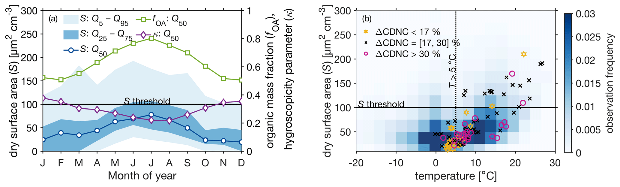
Figure 6 (a) The seasonal cycle of the dry aerosol size distribution surface area (S) calculated from the long-term aerosol size distribution observations (2012–2017; left y axis), where the markers represent the median values, the darkest shading represents the interquartile range, and the lighter shading represents the area between the 5th and 95th percentiles. Panel (a) also contains the median seasonal cycles of organic mass fraction and the κ hygroscopicity parameter compiled from the same long-term period (right y axis). The horizontal green line refers to the dry surface area threshold of 100 µm² cm⁻³ from Fig. 5, under which the greatest ΔCDNC are modeled using the BAECC data. (b) A density plot showing the observations of S under different ambient temperatures during the 2012–2017 long-term period. The S threshold of 100 µm² cm⁻³ is again shown with the horizontal green line. The vertical dashed green line is a rough estimate for the start of the thermal growing season, which also refers to the starting point of the majority of the BVOC emissions. The markers show the PARSEC–UFO simulation data color-coded with the associated ΔCDNC (simulations yielding the ΔCDNC below the 25th percentile are shown in blue, simulations yielding ΔCDNC above the 75th percentile are shown in red, and the simulations between those limits are shown in white).

Figure 6b shows the dry PNSD surface area derived from the long-term PNSD measurements at SMEAR II as a function of temperature. When the ambient temperature exceeds 5 °C, the dry PNSD surface area starts to increase with increasing temperature. The dry PNSD surface areas and ambient temperatures (from 8.4 m height; Fig. 1c) from the BAECC simulation period are also shown to highlight the fact that the BAECC sample represents well the long-term statistics of the thermal growing season, providing confidence in the representativity of the BAECC sampling period for this boreal environment. The BAECC samples are color-coded by the modeled ΔCDNC. The highest ΔCDNC values (i.e., ΔCDNC > 40 %) are modeled when the dry PNSD surface areas are below the 100 µm² cm⁻³ threshold. Importantly, most of these model scenarios yielding ΔCDNC > 40 % coincide with ambient temperatures between 5 and 8 °C; i.e., at times when the monoterpene concentrations are not at their highest yet sufficient concentrations of organic vapor are still present to cause a large cloud response. Therefore, it can be concluded that the highest ΔCDNC due to co-condensation can be expected in thermal spring and fall. However, due to the seasonality in hygroscopicity and the slightly higher κ in spring and autumn (as opposed to summer; Fig. 6a) the likelihoods of obtaining s_max exceeding 0.2 % to yield significant ΔCDNC can be somewhat buffered due to hygroscopic growth.

Next, the frequency with which the PNSD criteria ($D_{\mathrm{2}}/D_{\mathrm{1}}<$ 6 and N₁> 1000 cm⁻³) are fulfilled in the long-term size distribution measurements is examined. For this purpose, the same 6-year PNSD data set collected at SMEAR II fitted with two log-normal size distributions (Hussein et al., 2005) is utilized. The percentage of times the criteria are met is shown in Fig. 7a. The highest frequencies (30 %–40 % of the time) are observed in April, May, and September, which correlates with a high new particle formation (NPF) frequency at the site (Nieminen et al., 2014; Dada et al., 2017). The monthly median size distributions fulfilling the criteria are shown in Fig. 7c. They all clearly exhibit the lack of a Hoppel minimum, similarly to PNSD_NUM, and suggest a potentially high impact of newly formed particles on cloud properties through co-condensation. However, future work should focus on understanding how frequently the measured PNSD_NUM are actually exposed to droplet activation, which would help us assess the likelihood of large CDNC enhancements taking place in reality. This is particularly important because NPF typically takes place in sunny, non-cloudy days, which provides time for the PNSD_NUM to evolve before exposed to cloud base and subsequent droplet activation. The results again clearly emphasize the need for accurate representation of aerosol size distributions and lifecycle in models (such as GCMs and ESMs) to account for the impacts of co-condensation and the strong seasonality to be expected in the magnitudes in ΔCDNC.

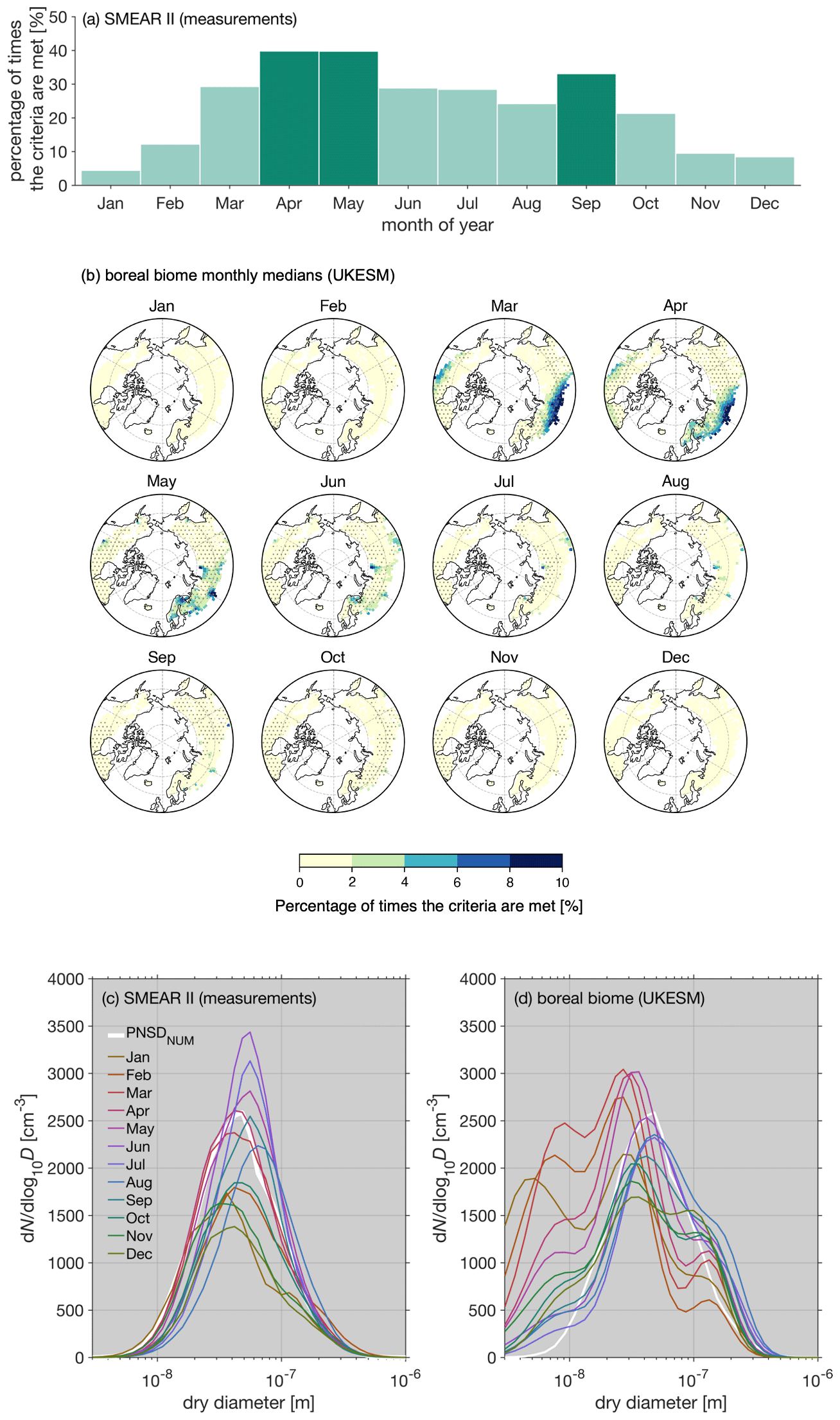
Figure 7 (a) Percentage of times the criteria ($D_{\mathrm{2}}/D_{\mathrm{1}}<$ 6 and N₁> 1000 cm⁻³) are met at SMEAR II between the 2012–2017 measurement period. D₂, D₁, and N₁ are attained from bimodal fits calculated for the measured PNSD using the Hussein et al. (2005) algorithm. (b) The percentage of times the criteria are met in a 2009–2013 UKESM1 simulation. D₂, D₁, and N₁ are the log-normal parameters representing the soluble accumulation mode and soluble Aitken modes. The gray markers refer to boreal grid cells, where the median updraft velocity at cloud base is between 0.2 and 0.5 m s⁻¹. (c–d) Monthly median size distributions from the long-term PNSD measurements at SMEAR II and UKESM1 simulation, respectively. The UKESM1 size distributions are calculated from the log-normal PNSD parameters for nucleation, soluble Aitken, and soluble accumulation modes, assuming geometric standard deviations of σ= 1.59 for nucleation and soluble Aitken modes and σ= 1.4 for the soluble accumulation mode. The soluble coarse mode is not included in the analysis.

3.5 Expected spatiotemporal variability in the impact of co-condensation on CDNC over the boreal biome

In this section, the SMEAR II results are compared against a 5-year UKESM1 simulation (see Sect. 2.4; analysis restricted to the boreal biome). While the SMEAR II PNSD data are retrieved at ground level, utilization of the UKESM1 modal parameters (only soluble modes considered) from CB is chosen because these PNSD log-normal parameters would actually meet the cloud droplet activation scheme in the model. Previous co-condensation parameterization schemes have also been developed to treat the CB PNSD to account for co-condensation (Connolly et al., 2014; Crooks et al., 2018). The monthly averages of the percentage of times the criteria ($D_{\mathrm{2}}/D_{\mathrm{1}}<$ 6 and N₁> 1000 cm⁻³) are fulfilled in the boreal grids are shown in Fig. 7b. Here, the Aitken mode geometric mean diameter and total number concentration (D₁, N₁) and accumulation mode geometric mean diameter (D₂) are obtained from the soluble Aitken and accumulation modal parameters (see Sect. 2.4 for more details regarding the UKESM1 modes). The frequencies, which remain roughly well below 6 %, are in general much lower than observed at SMEAR II. This can be explained by the lack of a boundary layer NPF process in the UKESM1 simulations (Sect. 2.4). Therefore, the UKESM1 results can be taken as the lower estimate. Figure 7d displays the monthly median PNSD in the boreal grid cells fulfilling the criteria ($D_{\mathrm{2}}/D_{\mathrm{1}}<$ 6 and N₁> 1000 cm⁻³), which are constructed from the soluble nucleation, soluble Aitken, and soluble accumulation mode modal parameters from the UKESM1 simulations when the criteria are fulfilled (criteria only uses soluble Aitken and soluble accumulation modes). The size distributions calculated using these UKESM1 modal parameters are in general less similar to the PNSD_NUM than the monthly median SMEAR II size distributions are (Fig. 7c) because they have more distinguished multimodal shapes, which arise from the modal representation of the PNSD. However, they still feature a minor accumulation mode in the presence of a large Aitken mode (with respect to N₁).

The UKESM1 results suggest that a strong spatiotemporal variability in the co-condensation-driven ΔCDNC should be expected if this process were to be represented in GCMs. Consistent with the SMEAR II observations (Fig. 7a), spring months stand out as the times when the criteria are most likely to be met, but the other peak in the frequency, expected in September at SMEAR II, cannot be seen. Another interesting feature is the large spatial variability in the frequency. In March and April, a very evident hotspot can be seen in the southern parts of the boreal forest, more precisely in the north of Kazakhstan. When the whole Northern Hemisphere is displayed, it is clear that the hotspot region extends over Europe during spring (Fig. S13) when the conditions favor the formation, growth, and survival of small particles (Kerminen et al., 2018), as shown in Fig. S14 in terms of nucleation mode number concentration. The result therefore suggests high co-condensation potential in areas rich in ultrafine particles. The cloud response of co-condensation in an extended domain covering most of Eurasia could be an interesting follow-up study. However, such a study should incorporate also the condensation of nitric acid and ammonia, the concentrations of which are presumably abundant in the regions where the co-condensation PNSD criteria are met (Kakavas et al., 2022). As this “Kazakhstan hotspot” is connected to aerosol phenomenology outside the boreal biome, the analysis is not continued further. Another evident springtime hotspot is located in North America, near the Rocky Mountains, but the updraft velocities at the area are not within the desired range ([0.2,0.5] m s⁻¹) to yield significant cloud response from co-condensation (Fig. 7b).

Aside from these hotspots, it is notable that the overall background of the frequency of the times the criteria are met in the latitude range of [0,75]° E increases from < 2 % to 2 %–6 % when moving from March to April. This background stays elevated until June. Smaller hotspots within this area are visible, and they correspond to regions known for high sulfur dioxide (SO₂) emissions, such as the Kola Peninsula. The Kola Peninsula SO₂ emissions have shown to trigger NPF events measured at SMEAR I in Finnish eastern Lapland (e.g., Kyrö et al., 2014). An interesting next step would be to see how Fig. 7b changes with UKESM1 simulations incorporating boundary layer NPF and whether the percentage of times the criteria are met increases to values comparable with the SMEAR II observations and whether the frequency becomes larger also in fall. Another interesting observation to be made from Fig. 7b is that no significant impact of co-condensation would be expected in UKESM1 in most of Siberia (east and northeastern Siberia), which can be explained by the lack of nucleation mode particles in the UKESM1 simulations over the region (Fig. S15).

4 Conclusions

This study focuses on the role of the co-condensation of organic vapor and water on warm cloud microphysics in a boreal forest environment. Co-condensation has been proposed as a potentially significant process contributing to the feedbacks between VOC emissions, SOA loadings, cloud formation, and climate. Boreal forests account for about a third of the Earth's forested area and are potentially significant sources of such co-condensing species.

First, PARSEC–UFO model is used to perform simulations for the BAECC measurement campaign which took place at the SMEAR II station in southern Finland during 2014 (Petäjä et al., 2016). The measurement setup during BAECC was very advanced, enabling the initialization of PARSEC–UFO with state-of-the art data describing the ambient aerosol physical and chemical properties. The measurements conducted with the FIGAERO–I-CIMS (e.g., Mohr et al., 2017) are of high importance for this study due to the simultaneous measurements of organic particle and vapor species. These data enable the incorporation of organic vapors from a broad volatility range into the PARSEC–UFO simulations. The previous modeling work on this topic used volatility distributions based on particle-phase measurements only, resulting in overall lower volatility and contributions of semi- and intermediate-volatility organic vapor.

The results from the PARSEC–UFO simulations reveal that a competition effect exists between the reductions in maximum supersaturations and critical supersaturations needed for aerosol particle activation into cloud droplets when co-condensation is considered. The reductions in critical supersaturations are greater than the reductions in maximum supersaturation, which results in the simulated CDNC enhancements (simulations with co-condensation are compared against simulations without it under same meteorological conditions). The CDNC enhancements are of the order of 20 % under realistic updraft velocities (0.1, 0.3, and 1 m s⁻¹) and correspond to reductions of 10–16 nm in the smallest activated dry diameters (∼ 144 to ∼ 128, ∼ 102 to ∼ 88, and 72 to ∼ 62 nm for the 0.1, 0.3, and 1 m s⁻¹ updraft scenarios, respectively). The activation of smaller particles into cloud droplets results, as expected, in the formation of more numerous smaller cloud droplets. The critical supersaturation reductions result from the additions of soluble organic mass below cloud base along the simulated air parcels' adiabatic ascents, while the reductions in maximum supersaturation are caused by the increasing condensation sink provided by more cloud droplets (the source of supersaturation is fixed as the meteorological conditions between simulations with and without co-condensation are kept constant).

The predicted CDNC enhancements are highest for the 0.3 m s⁻¹ updraft velocities and depend on several, at least partly, interlinked parameters (see also Lowe et al., 2019). One parameter affecting the modeled CDNC is the availability of the co-condensable organic vapors, which in turn depends on the updraft velocities, the features of the organic volatility distribution, as well as initial temperature and relative humidity. Most organic vapor condenses under the slowest adiabatic ascents and least in the highest due to kinetics. The organic volatility bins spanning from ELVOCs to the lower-volatility IVOCs condense in a similar, updraft-dependent, degree prior reaching the cloud base. Organic vapors of higher volatility involving species such as formic acid condense less efficiently, and their condensation is sensitive to the presence of large particles which are likely to activate regardless of co-condensation. Therefore, small enhancements in particularly SVOC and lower-volatility IVOC concentrations lead to significant enhancements in CDNC, while increases in the most volatile IVOCs and formic acid do not affect CDNC much.

The simulations performed with 0.3 m s⁻¹ updrafts are repeated using volatility distributions from previous co-condensation studies (Cappa and Jimenez, 2010; Topping et al., 2013; Crooks et al., 2018). By doing so, the BAECC campaign median CDNC enhancement decreased from 22 % ∼ to non-significant values. This result is explained by the lower initialization temperature regulating organic vapor availability, as well as lower SVOC and IVOC concentrations in previous studies, highlighting the added value of capturing these higher-volatility bins within the VBS representations of atmospheric organic species. On the other hand, adding information on the LVOC and ELVOC range does not significantly influence the CDNC enhancements due to co-condensation.

The sensitivity of the modeled ΔCDNC to organic vapor concentrations is strongest when high maximum supersaturations ($s_{max}>$ 0.2 % for the 0.3 m s⁻¹ updraft scenarios) are reached. Such conditions are achieved when the dry PNSD surface area (a proxy for the condensation sink) remains below 100 µm² cm⁻³. Under those conditions, CDNC enhancements exceeding 40 % are predicted for conditions in which roughly 1 µg m⁻³ of co-condensable organic vapor is present.

Besides the meteorological conditions and the availability of co-condensable vapors, the CDNC enhancements depend critically on the size distribution of the initial aerosol population. Highest CDNC enhancements are generally achieved when the model is initialized with a relatively small accumulation mode combined with a large nascent ultrafine particle mode with a geometric mean diameter of ca. 40 nm and with no visible Hoppel minimum present in the distribution. Such conditions are observed most frequently in spring and September (about 30 %–40 % of the time in years 2012–2017), when new particle formation events take place at SMEAR II.

Subsequently, UKESM1 simulations (years 2009–2013) are utilized to investigate the potential impact of including the process of co-condensation on droplet formation in this model over the whole boreal biome using the criteria developed from the SMEAR II case to identify most susceptible PNSD conditions. Overall, the UKESM1 PNSD are different from those observed at SMEAR II, even when the strict criteria are used to select the ideal PNSD for co-condensation-driven enhancements in CDNC. This discrepancy can arise from multiple causes such as the lack of critical aerosol processes (boundary layer new particle formation), but it could also be a common ESM feature arising from the modal representation of PNSD. Nonetheless, aside from two hotspots (one near the Rocky Mountains in North America and one over northern Kazakhstan, which are not analyzed further), the presence of suitable PNSD, as experienced by UKESM1, is most frequent over Fennoscandia and western parts of Siberia in spring, yet the frequencies at which those PNSD are modeled remained much lower than those obtained from the long-term SMEAR II PNSD measurements (2 %–6 % in UKESM1). Perhaps surprisingly, suitable PNSD are never modeled over most of Siberia, suggesting that for the model configuration of UKESM1 used in this study, the process of co-condensation would not be expected to have an influence on droplet formation in this area. This is due to the low concentration of ultrafine particle particles modeled in the area.

In summary, these results highlight the potential significance of co-condensation in pristine boreal environments with a nascent ultrafine particle mode present. Such conditions are met over Fennoscandia and the western parts of Siberia in spring, and to a lesser extent in the fall, when NPF takes place. For future modeling purposes, it is vital to stress the importance of the accurate representation of PNSD for capturing the role of the co-condensation of organics in CDNC enhancements, including appropriate descriptions of the boundary layer NPF. Because the modeled CDNC enhancements are so significant, further research focus, especially regarding observations of the co-condensation, should be targeted in the future to motivate future assessments of co-condensation-driven radiative forcing. Perhaps this work inspires aircraft measurements (of the relevant parameters discussed in this paper) over Fennoscandia in the future to finally narrow down the importance of co-condensation for the accurate representation of CDNC in GCMs.

Appendix A

The effect of the initialization relative humidity, organic mass accommodation coefficient (α_Org), and vaporization enthalpy (ΔH_VAP) on the modeled CDNC enhancements due to co-condensation are investigated for three different conditions (simulation ID nos. 13, 55, and 95, respectively; Table S1). The three conditions were selected, as they are representative of low, median, and high ΔCDNC simulated during BAECC. Table A1 describes the simulation setup for this sensitivity study.

Table A1 The simulation setup for studying the sensitivities of initialization RH organic mass accommodation coefficient (α_Org) and vaporization enthalpy (ΔH_VAP) on ΔCDNC is shown. Three simulation IDs are selected from the BAECC campaign (nos. 13, 55, and 95, respectively; Table S1), and three simulation sets (for varying initialization RH, α_Org and ΔH_VAP, respectively) are performed for each ID with and without co-condensation. The initial temperature, aerosol chemical composition, and PNSD vary between the different IDs and are taken from Table S1. A fixed updraft velocity of 0.3 m s⁻¹ is applied for all the different simulations.

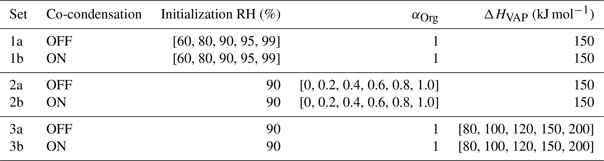
The initialization RH affects the availability of organic vapor for co-condensation; when PARSEC–UFO is initialized under high RH (≳ 95 %), most organic vapor is scavenged at initial conditions, causing negligible enhancements in the CDNC. On the other hand, if the initialization RH is lower (< 90 %), less organic vapor is scavenged at initial conditions, and the modeled ΔCDNC values are greater (Fig. A1). By varying α_Org, the effect that the assumption of ideality has on the projected CDNC enhancements is probed. For simplicity, the mass accommodation coefficient for organics (α_Org) is set to be constant across the volatility bins. By reducing α_Org from 1 to 0.8, the condensation of organics reduces. However, this impacts CDNC only in simulation ID no. 95 (Fig. A2; CDNC reduces from ∼ 62 % to 55 %), i.e., simulation with the highest ΔCDNC. When α_Org< 0.4, simulation ID no. 55 also shows a reduction in the modeled ΔCDNC as it drops from ∼ 22 % to ∼ 15 %. The selection of the enthalpy of vaporization for organics does not affect ΔCDNC (Fig. A3). Over all, the initial relative humidity plays the most critical role out of the three parameters considered here (RH, α_Org, and ΔH_VAP) on the modeled ΔCDNC.

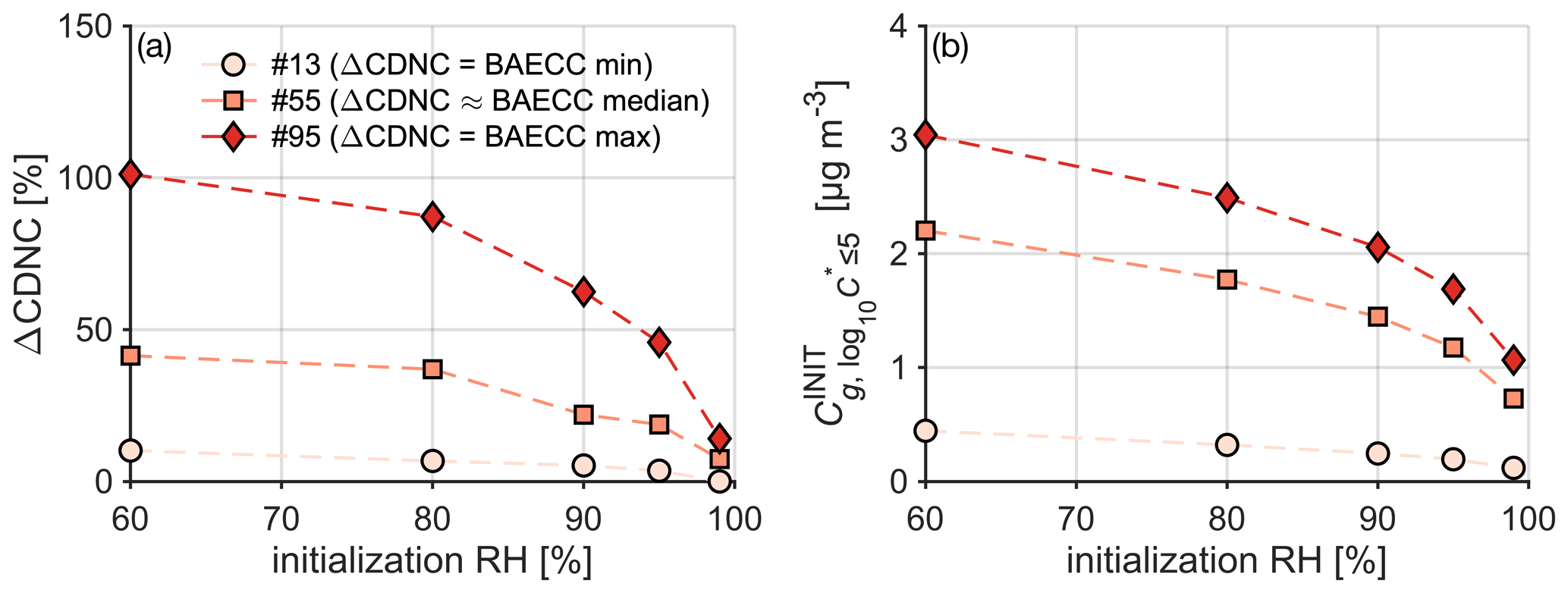
Figure A1 The modeled CDNC enhancements as a function of initialization RH ranging from 60 % to 99 % (indicated with different colors) for each simulation ID are shown, respectively. The initialization temperature and pressure are fixed to values shown in Table S1, and only the volatility bins ${\log }_{\mathrm{10}}{C}^{*}\le$ 5 are included, which is motivated, e.g., by Fig. 4. The simulations are performed with an updraft velocity of 0.3 m s⁻¹. The markers with the lightest color refer to the BAECC simulation, where co-condensation influenced ΔCDNC negligibly (ID no. 13; ΔCDNC = 3 %). The orange markers refer to the BAECC median ΔCDNC (ID no. 55), and the red markers represent a simulation, where the modeled ΔCDNC was greatest (ID no. 95; ΔCDNC = 75 %). ΔCDNC is calculated 50 m above CB based on critical radii, similar to the study.

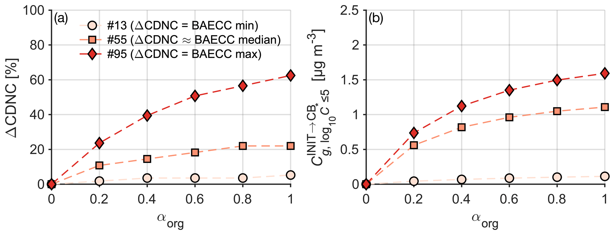
Figure A2 The modeled CDNC enhancements as a function of mass accommodation coefficient for organics (α_Org) ranging from zero to one. The colors and presented simulations are same as in Fig. A1.

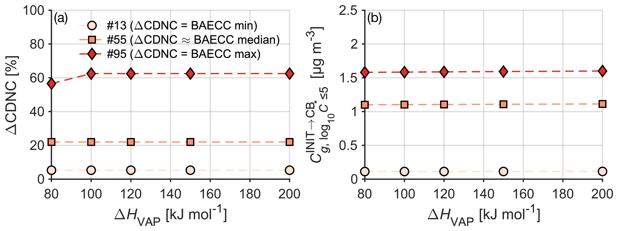
Figure A3 The modeled CDNC enhancements as a function of vaporization enthalpy for organics (ΔH_VAP) ranging from zero to one. The colors and presented simulations are same as in Fig. A1.