Consistency evaluation of tropospheric ozone from ozonesonde and IAGOS (In-service Aircraft for a Global Observing System) observations: vertical distribution, ozonesonde types, and station–airport distance

The vertical distribution of tropospheric O₃ from ozonesondes is compared with that from In-service Aircraft for a Global Observing System (IAGOS) measurements collected at 23 pairs of sites between about 30° S and 55° N from 1995 to 2021. Profiles of tropospheric O₃ from IAGOS are generally in good agreement with ozonesonde observations from electrochemical concentration cells (ECCs), Brewer–Mast sondes, and carbon–iodine sensors, with average biases of 2.58, −0.28, and 0.67 ppb and correlation coefficients (R) of 0.72, 0.82, and 0.66, respectively. Agreement between aircraft and Indian-sonde observations is poor, with an average bias of 15.32 ppb and an R value of 0.44. The O₃ concentration observed by ECC sondes is, on average, 5 %–10 % higher than that observed by IAGOS, and the relative bias increases modestly with altitude. For other sonde types, there are some seasonal and altitudinal variations in the relative bias with respect to the IAGOS measurements, but these appear to be caused by local differences. The distance between the station and airport, when within 4° (latitude and longitude), has little effect on the comparison results. For the ECC ozonesondes, the overall bias with respect to the IAGOS measurements varies from 5.7 to 9.8 ppb when the station pairs are grouped by station–airport distances of <1° (latitude and longitude), 1–2°, and 2–4°. Correlations for these groups correspond to R=0.8, 0.9, and 0.7. These comparison results provide important information for merging ozonesonde and IAGOS measurement datasets. They can also be used to evaluate the relative biases of different sonde types in the troposphere, using the aircraft as a transfer standard.

1 Introduction

Ozone (O₃) is a trace gas with small concentrations in the atmosphere (Ramanathan et al., 1985). It is an important greenhouse gas in the upper troposphere. In the planetary boundary layer, it is a major air pollutant (Lefohn et al., 2018; Monks et al., 2015). It can endanger human health, damage ecosystems, and affect climate change (Fu and Tai, 2015; Lefohn et al., 2018; Percy et al., 2003). Therefore, it is important to study the temporal and spatial variations in tropospheric O₃, including near-surface O₃, and mechanisms affecting the variations (Logan, 1985; Ma et al., 2020; Sharma et al., 2017; Young et al., 2018).

A large number of studies have been carried out on the spatiotemporal distribution, formation mechanisms, and transport characteristics of tropospheric O₃ (Li et al., 2020, 2021; Vingarzan, 2004; Wang et al., 2017, 2023; Xu et al., 2021; Yu et al., 2021). However, due to the limitations of observations, there are many unknowns regarding tropospheric O₃, especially its vertical distribution. Satellites provide an effective platform for measuring O₃ globally. Satellite O₃ instruments, including the Tropospheric Emission Spectrometer (TES), the Global Ozone Monitoring Experiment (GOME), GOME-2, SCIAMACHY, the Ozone Monitoring Instrument (OMI), and the TROPOspheric Monitoring Instrument (TROPOMI), have been in operation for decades (David and Nair, 2013; Ebojie et al., 2016; Hegarty et al., 2009; Hoogen et al., 1999; Hubert et al., 2021; Miles et al., 2015). Although satellite observations can provide detailed temporally and horizontally resolved maps of tropospheric O₃ columns, in general, satellite data lack a sufficient vertical resolution. While tropospheric differential-absorption lidar can also provide vertical-distribution information pertaining to tropospheric O₃ (Keckhut et al., 2004; Yang et al., 2023), there are very few routinely operating stations.

The principal sources of vertically resolved, trend-quality observations of tropospheric O₃ are therefore balloon-borne ozonesondes and In-service Aircraft for a Global Observing System (IAGOS) observations. The World Ozone and Ultraviolet Radiation Data Centre (WOUDC) and IAGOS databases house data from these two observation programmes, which have the longest durations and the most global stations, making them the most widely used programmes for tropospheric O₃ studies (Gaudel et al., 2020; Liao et al., 2021; Tarasick et al., 2019; Wang et al., 2022; Zang et al., 2024). These two datasets are used to study the distribution, variability, and trends of tropospheric O₃, as well as its sources and transport, along with satellite and model validation (Hu et al., 2017; Gaudel et al., 2018; 2020; Wang et al., 2022; Zhang et al., 2008). The first phase of the Tropospheric Ozone Assessment Report (TOAR-I), initiated in 2014, utilized available surface, ozonesonde, aircraft, and satellite observations to assess tropospheric O₃ trends from 1970 to 2014 (Schultz et al., 2017). Hu et al. (2017) found that the largest bias in the chemical transport model GEOS-Chem, with respect to ozonesondes and IAGOS observations, occurs at high northern latitudes in winter–spring, where the simulated O₃ is 10–20 ppb lower. Wang et al. (2022) examined observed tropospheric O₃ trends, their attributions, and radiative impacts from 1995 to 2017 using aircraft observations from IAGOS, ozonesondes, and a multi-decadal GEOS-Chem chemical-model simulation and found that IAGOS observations over 11 regions in the Northern Hemisphere and at 19 of the 27 global ozonesonde sites showed measured increases in tropospheric ozone (950–250 hPa) of 2.7±1.7 and 1.9±1.7 ppbv per decade on average, respectively.

There are also a number of comparative studies on these two datasets (Zbinden et al., 2013; Staufer et al., 2013, 2014; Tanimoto et al., 2015; Tarasick et al., 2019). Staufer et al. (2013, 2014) used trajectory calculations to match air parcels sampled by both sondes and aircraft. Zbinden et al. (2013) compared coincidences (±24 h) at three pairs of sites, while Tanimoto et al. (2015) examined simultaneous observations (±3 h for sondes versus aircraft) at several pairs of sites less than 100 km apart. In general, these studies show small (6 % or less) negative biases in aircraft measurements compared to electrochemical-concentration-cell (ECC) sondes. Tarasick et al. (2019) compared trajectory-mapped averages over ozonesonde and MOZAIC–IAGOS (Measurements of OZone and water vapour by in-service AIrbus airCraft–IAGOS) profiles across 20–70° N and concluded that, over the period from 1994–2012, ozonesonde measurements were about 5±1 % higher in the lower troposphere and 8±1 % higher in the upper troposphere.

As shown above, the global O₃ vertical-distribution datasets observed by the WOUDC and IAGOS have been widely used in various studies. However, long-term and multi-site systematic comparisons of these two datasets are rare, especially for observations from the past 3 decades. In this study, we attempt to provide the most comprehensive evaluation to date of the relative biases in IAGOS and sonde profiles, using as many station pairs as possible. We identify 23 suitable pairs of sites in the WOUDC and IAGOS datasets from 1995 to 2021, compare the average vertical distributions of tropospheric O₃ shown by ozonesonde and aircraft measurements, and analyse their differences based on ozonesonde type and station–airport distance.

2 Data and methods

2.1 MOZAIC–IAGOS observations

The MOZAIC (Measurements of OZone and water vapour by in-service AIrbus airCraft) programme, initiated in 1994 and incorporated into the IAGOS (In-service Aircraft for a Global Observing System) programme (https://www.iagos.org, last access: 27 September 2024) in 2011, takes advantage of commercial aircraft to provide worldwide in situ measurements of several trace gases (e.g. O₃ and CO) and meteorological variables (e.g. water vapour) obtained throughout the troposphere and the lower stratosphere (Marenco et al., 1998; Petzold et al., 2015; Nédélec et al., 2015). O₃ measurements are performed using a dual-beam UV-absorption monitor (time resolution of 4 s) with an instrumental uncertainty of ±2 ppbv +2 % (Thouret et al., 1998; Blot et al., 2021). It should be noted that this is only the instrumental uncertainty and does not include sampling uncertainties (possible losses) caused by the inlet line and the compressor before the UV-photometer measurements are made. Loss of O₃ on the inlet pump was an issue in earlier aircraft-based O₃ sampling programmes (Brunner et al., 2001; Dias-Lalcaca et al., 1998; Schnadt Poberaj et al., 2007; Thouret et al., 2022), but Thouret et al. (1998) found this to be negligible for MOZAIC–IAGOS.

More details on the new IAGOS instrumentation can be found in Nédélec et al. (2015). The continuity of the dataset between the MOZAIC and IAGOS programmes has been demonstrated based on their 2-year overlap (2011–2012) (Nédélec et al., 2015). Blot et al. (2021) evaluated the internal consistency of the O₃ measurements collected since 1994, which confirmed the instrumental uncertainty of ±2 ppb. Moreover, they found no bias drift among the different instrument units (six O₃ MOZAIC–IAGOS instruments, nine IAGOS-CORE Package1 instruments, and the two instruments used on the IAGOS-CARIBIC aircraft).

2.2 WOUDC ozonesonde observations

The World Ozone and Ultraviolet Radiation Data Centre (WOUDC) is part of the Global Atmosphere Watch (GAW) Programme of the World Meteorological Organization (WHO; https://woudc.org/data/explore.php, last access: 27 September 2027). The WOUDC is operated by Environment and Climate Change Canada. WOUDC ozonesonde data have been evaluated in a number of international WMO-sponsored field intercomparisons (Attmannspacher and Dütsch, 1970, 1981; Kerr et al., 1994) and, more recently, in laboratory simulation chamber experiments using a standard reference photometer (Smit et al., 2007, 2024; Thompson et al., 2019). In the global ozonesonde network, while different ozonesonde types were common in the past, more than 95 % of current sounding stations use electrochemical concentration cells (ECCs). ECC ozonesondes have a precision of 3 %–5 % (1σ), while the precision of other sonde types is somewhat poorer (about 5 %–10 %) for Brewer–Mast and Japanese KC (carbon–iodine) sondes and somewhat larger for Indian sondes (Kerr et al., 1994; Smit et al., 2007). Biases with respect to UV reference spectrometers have been estimated as ranging from 1 %–5 % for ECC sondes in the troposphere (Smit et al., 2021; Tarasick et al., 2019, 2021).

Table 1 Summary of the station information, including the name, geolocation, number of profiles, observational period, and station–pair distance corresponding to each station used in this study.

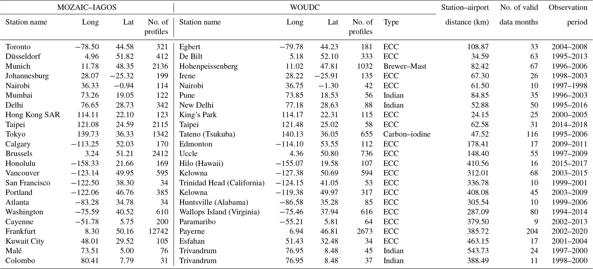
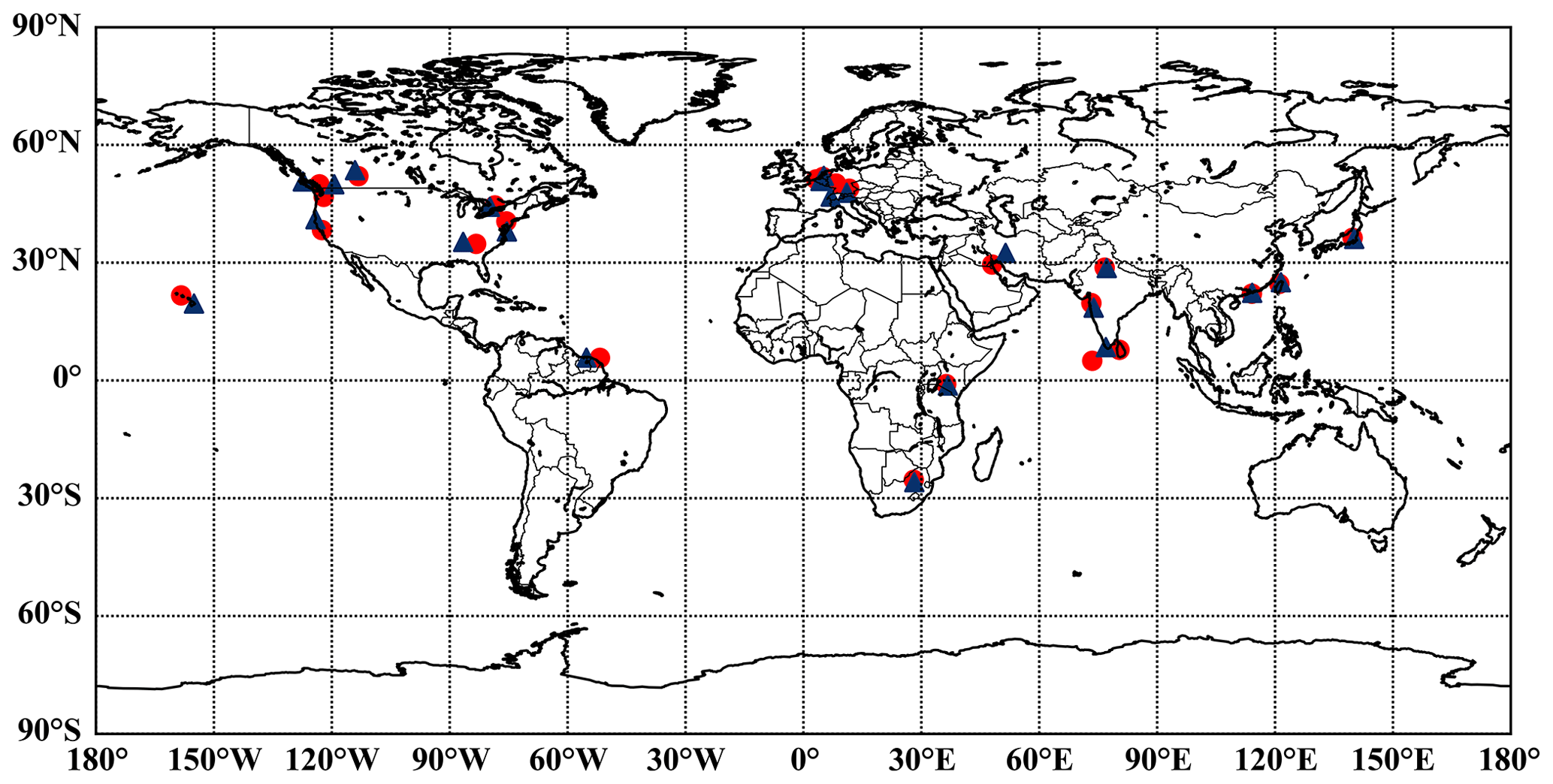
Figure 1 Map of the 23 pairs of sites used in this study. Circular red markers represent the IAGOS sites, while triangular blue markers represent the WOUDC sites.

2.3 Data processing

The two datasets were first screened for airport-sonde station pairs within a latitudinal separation of <4° and a longitudinal separation of <4°. Many sonde stations have observational records that do not overlap with the IAGOS period (1994–present). In addition, the IAGOS dataset has large gaps for many airports because the frequency of visits to airports by aircraft participating in IAGOS depends on the operating constraints of commercial airlines. In total, 23 station pairs (Fig. 1) were identified as having a separation of less than 4° in both latitude and longitude, with coincident observations obtained over at least 9 months. The majority of the 23 ozonesonde site records pertain to ECCs (17), while four correspond to Indian sondes, one corresponds to Brewer–Mast sondes, and one pertains to carbon–iodine sondes (Japanese KC sondes). These stations were divided into three groups according to the distance (D) between the ozonesonde station and the airport: D<1°, $\mathrm{1}\mathit{°}<D<\mathrm{2}\mathit{°}$, and $\mathrm{2}\mathit{°}<D<\mathrm{4}\mathit{°}$. Specific information on the comparison stations is shown in Table 1.

The observation times of the ozonesondes and aircraft are generally not the same. Ozonesondes are typically launched once a week, although a few stations have more frequent launches. The aircraft records generally contain more frequent observations, but the observation times vary. For the 23 selected stations, we calculated the mean O₃ vertical profiles at a 1 km resolution (with the first layer extending from the surface to 1 km above sea level) for each month during the observational period for the two datasets. A minimum of four aircraft profiles were required to estimate the monthly mean profiles; however, because ozonesonde launches typically only occur a few times per month, no minimum was required to estimate the monthly mean profiles. Only data with monthly means in both datasets were included for further analysis. Comparisons between the two datasets were made based on ozonesonde type and station–airport distance.

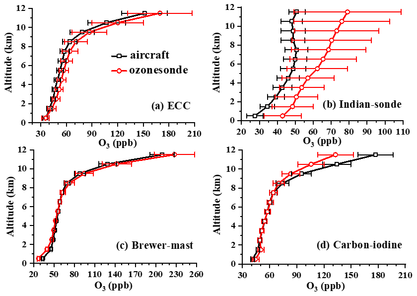
Figure 2 Comparison of the vertical profiles of tropospheric O₃ observed from aircraft measurements and four types of ozonesondes (ECC, Indian, Brewer–Mast, and carbon–iodine sondes). The error bar length is 4 times the standard error (SE) of the mean (equivalent to the 95 % confidence limits for the averages).

3 Results and discussion

3.1 Comparison of the vertical profiles of tropospheric O₃ from four types of ozonesondes and aircraft observations

Previous intercomparisons of sondes launched from the same balloon (Attmannspacher and Dütsch, 1970, 1981; Beekmann et al., 1994, 1995; Deshler et al., 2008; Hilsenrath et al., 1986; Kerr et al., 1994; Smit et al., 2007) have shown that sondes of different types respond somewhat differently to the same O₃ vertical profile; that is, they have relative biases that vary with altitude. Figure 2, therefore, compares the mean vertical profiles of tropospheric O₃ from ozonesonde and aircraft measurements, separated by ozonesonde type. Both O₃ concentrations and absolute differences between ozonesondes and aircraft increase with altitude, especially above 9 km. Average tropospheric O₃ profiles observed by ECCs, Brewer–Mast sondes, and carbon–iodine sondes are in good agreement with aircraft measurements, with biases of 2.58, −0.28, and 0.67 ppb, respectively, while the agreement with Indian sondes is poorer, with a bias of 15.32 ppb. The average of the Indian sondes also shows a linear increase with altitude, while the aircraft measurements indicate an O₃ decrease with altitude above 8 km (Fig. 2b). This behaviour is most clearly related to comparisons made in spring between stations located 2–4° apart (Fig. S9 in the Supplement).

These results are broadly consistent with those from JOSIE 1996 (Smit et al., 1996; Smit and Kley, 1998; Thompson et al., 2019) and with the Northern-Hemisphere-averaged results from Tarasick et al. (2019). (Note that Fig. 20b in Tarasick et al. (2019) is largely based on ECC sondes and that the scale is inverted (IAGOS–sondes) compared to the one we use here.)

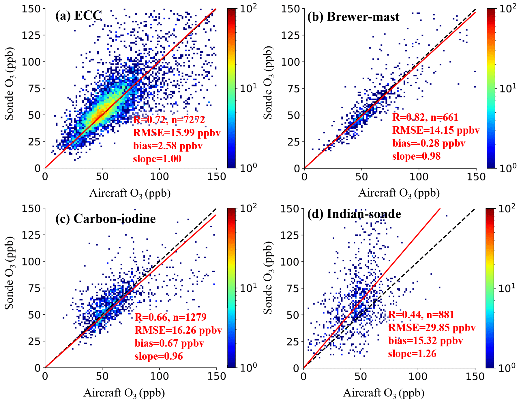
Figure 3 Correlation (R) of monthly mean ozone mixing ratios between ozonesonde and aircraft measurements. While IAGOS does record measurements in the lower stratosphere, these values are usually obtained far from the airport, meaning the sonde–aircraft distance is large. Therefore, we only plot data below 150 ppb. The dashed black line shows the 1:1 axis, the red line shows the linear fit (with the intercept set to 0), and the colour bar shows the data counts. Correlations are significant at the 99 % confidence level (p<0.01). N denotes the number of data points, R is the correlation coefficient, bias corresponds to the overall average difference in monthly mean values (ozonesonde ozone minus aircraft ozone (measured in ppb)), RMSE is the root mean square error, and the slope is the slope of the linear fit line. All data points are based on the monthly mean.

Figure 3 shows correlation plots of monthly mean O₃ at 1 km vertical intervals for months when both IAGOS and ozonesonde data were available at the same location. While these monthly averages are from data that are not necessarily coincident in time, Fig. 3a–c indicate that the data compare well on this timescale, with correlation coefficients (R) of 0.71, 0.88, and 0.66, respectively. The agreement between Indian-sonde and aircraft observations is poor, however, with an R value of only 0.44 (Fig. 3d). The root mean square errors (RMSEs) of O₃ for the four types of ozonesondes (ECC, Brewer–Mast, carbon–iodine, and Indian sondes) and the aircraft are 15.99, 14.15, 16.26, and 29.85 ppb, respectively. After calculation, we obtained the slopes and offsets for the ECC, Brewer–Mast, carbon–iodine, and Indian sondes without forcing the fitted lines through zero. The slopes are 0.71, 0.88, 0.56, and 0.74, and the offsets are 18.94, 6.89, 27.48, and 27.84 ppb, respectively. When we force the intercept to zero for the regressions, the slope becomes larger than when the fitted lines are not forced through zero (Fig. 3). Generally, when O₃ is zero, both the ozonesondes and the aircraft will record a measurement of zero. However, there is an offset in the fit of the two datasets due to potential causes of systematic differences during the observation measurement process, e.g. a high background current in the sonde data.

Figure 2 shows that the mean differences between ozonesonde and aircraft measurements vary significantly with altitude. This can also be observed clearly from the relative differences (RDs), expressed as (O_3-ozonesonde – O_3-aircraft)/O_3-aircraft×100 % (Fig. 4). O₃ concentrations from ECC measurements are higher than those from aircraft measurements at all altitudes (except at the surface). Mean O₃ concentrations reported by Brewer–Mast sondes are lower than those from IAGOS below 7 km altitude, but they are higher between 7 and 12 km altitude. O₃ concentrations reported by carbon–iodine sondes are higher than those observed by aircraft below 2 km altitude, but they are significantly lower above 8 km altitude. In relative terms, the bias between ECC sonde measurements and aircraft measurements varies little with altitude, except near the ground. The mean relative bias for Brewer–Mast sonde measurements is at an absolute maximum of −19 % near the ground but increases slowly above 3 km altitude and is positive above 7 km altitude, reaching more than +10 % at altitudes of 10–11 km. The relative bias for carbon–iodine measurements is about 8 % below 2 km altitude, becomes quite small from 2–8 km altitude, and becomes large and negative above 8 km altitude.

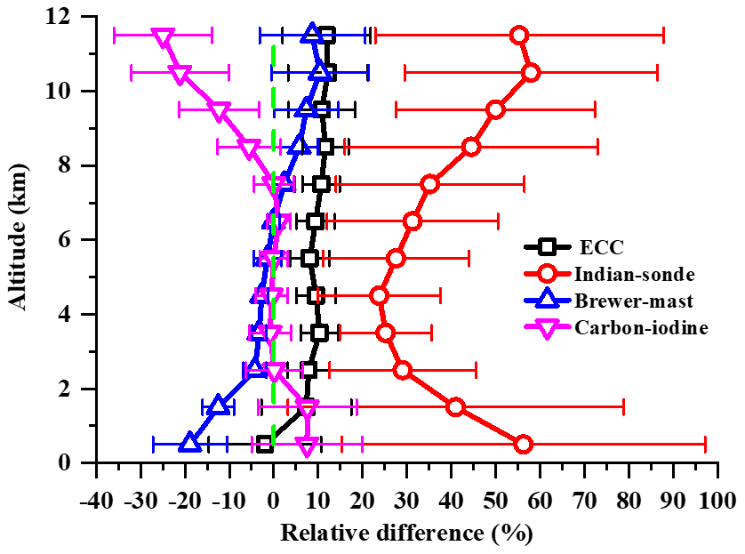
Figure 4 Mean relative difference (RD) between the ozonesonde O₃ and aircraft O₃ data. The RD is calculated using the formula (O_3-ozonesonde – O_3-aircraft)/O_3-aircraft×100 %. The dashed green line represents the zero line.

The Indian-sonde observations show much larger mean differences than the aircraft measurements. The biases are consistently positive, reaching as high as nearly 60 % or 30 ppb, with much higher uncertainty (standard errors) at each altitude as well (Figs. 2b, 4).

The region below 3 km altitude has many local ozone sources and sinks (cities, airports, rural environments, etc.). In comparison, the region above 8 km altitude is significantly influenced by stratosphere–troposphere exchange, jet streams, and tropopause folds. Figure S1 in the Supplement shows that the correlation coefficient (R) between ozonesondes and aircraft observations is higher near the ground (<2 km) and at high altitudes (>10 km). This shows that although the influencing factors of O₃ near the ground and at high altitudes are more complex, their long-term temporal-variation characteristics are similar. The influences of cities, airports, rural environments, stratosphere–troposphere exchange, jet streams, tropopause folds, etc., have a more significant impact on the concentration of O₃ in the short term.

The correlation between the four types of ozonesondes and aircraft observations also varies with altitude (Fig. S1). From 0–8 km, the correlation between ECC and aircraft observations decreases with altitude, with R corresponding to 0.71 at 0–1 km altitude and reaching a minimum of 0.29 at 8–9 km altitude. From 8–12 km, R increases with altitude, reaching 0.49 at altitudes of 11–12 km. The correlation between the other three ozonesondes (i.e. the Brewer–Mast, Indian, and carbon–iodine ozonesondes) and the aircraft observations also varies with altitude, exhibiting different inflection points. The number of stations for these three types of ozonesondes is small (Table 1). Therefore, local variable influences on O₃ are more important, meaning R varies more with altitude.

The bias and RMSE with respect to the aircraft observations of the four types of ozonesondes at 8–12 km altitude are higher than those at other altitudes. In contrast, the bias and RMSE values pertaining to altitudes below 8 km are smaller and vary less with altitude, consistent with the vertical-distribution characteristics of O₃ concentration shown in Fig. 2. This is likely due to the higher concentration of O₃ and the typically larger difference in spatial distance between ozonesonde and aircraft observations at 8–12 km altitude.

In addition, the bias and RMSE relative to the aircraft observations obtained at different altitudes for the ECC, carbon–iodine, and Brewer–Mast sondes are lower than those for the Indian sondes, which is consistent with the results of the previous analysis of O₃ concentration.

It should be noted that these comparisons only provide the average relative bias between the sondes and IAGOS. The true value of the ozone profile remains unknown, as do the absolute biases of the sondes and IAGOS.

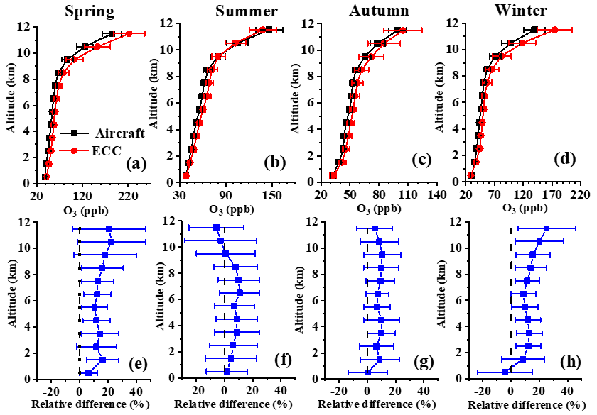
Figure 5 The mean difference in vertical profiles of tropospheric O₃ between ECC ozonesonde and aircraft observations with respect to the four seasons (a–d) and the corresponding mean relative differences. The dashed black line represents the zero line (e–h).

3.2 Seasonal variations in relative biases between ozonesondes and IAGOS

Figure 5 compares the mean profiles observed by the ECC ozonesondes and IAGOS, separated by season. There are modest seasonal differences in the relative-bias profiles, with somewhat larger average biases for winter and spring, but the average biases are all positive (with ECC sondes reporting higher values), and at all levels, the average seasonal biases are not statistically different.

The modest seasonal differences that are apparent in Figs. 5 and S2–S4 are likely due to the modest sample size for ECC sondes and the small sample sizes for the other types. The actual coincidence in time for the profiles can range from less than 1 day to about 1–3 weeks, depending on the number of ozonesonde and aircraft O₃ profiles collected within each month bin. This means the larger the atmospheric variability in O₃, the larger the real differences between ozonesonde and aircraft O₃ can become, particularly when the number of profiles within a month bin is small. In addition, there are errors due to variations in the aircraft take-off and landing trajectories, variations in the balloon rise rate, the geographical locations of the observation stations (and any associated meteorological differences), and any systematic differences in standard observational times.

Table 2 The bias, correlation coefficient (R), and RMSE for four types of ozonesonde and aircraft observations with respect to the four seasons.

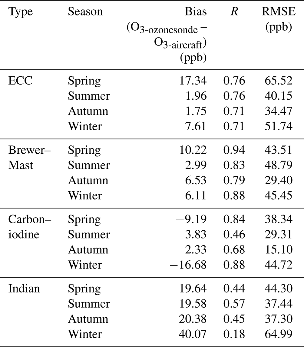
Table 2 indicates that in all four seasons, ECC data correlate well with aircraft observations, with R ranging from 0.71 to 0.76. However, there are larger average biases in winter and spring, as previously noted. It is not clear whether these seasonal-average differences in bias are significant as the uncertainty ranges for the seasonal averages (Fig. 5e–h) overlap.

The vertical distribution of tropospheric O₃ observed by Brewer–Mast sondes and IAGOS in the four seasons is similar (Fig. S2 in the Supplement). The differences are also similar, except above 7 km altitude, where the uncertainties are larger and, in general, the uncertainty ranges for the seasonal-average differences overlap. Since these comparisons come from only one station pair, some of the differences may be attributable to local differences in topography and meteorology. Table 2 shows that correlations for the single Brewer–Mast station are higher than those for ECC stations. Like the ECC sondes, the average biases are all positive, but this is determined by the biases above 7 km altitude (Fig. 4); unlike the ECCs, the biases are negative at the lowest 3 km of altitude.

The vertical distributions of tropospheric O₃ concentrations observed by carbon–iodine sondes and IAGOS in the four seasons are similar, except in summer, when the tropopause is high (Fig. S3 in the Supplement). The difference plots are fairly similar, except at the lowest 3 km of altitude, where differences become quite large in summer. Like the previous comparison for Brewer–Mast sondes, these comparisons come from only one station pair, meaning the large differences in the boundary layer during summer are likely due to local O₃ production sampled by the sonde (but not the aircraft). This is likely the reason why the correlation between carbon–iodine and aircraft observations is poor in summer, with R only reaching 0.46 (Table 2). For the other three seasons, the correlation is fairly good.

The tropospheric O₃ observed by Indian sondes displays a consistently high bias relative to IAGOS in all seasons, and the seasonal difference plots are quite similar, except at the lowest 3 km of altitude in winter (Fig. S4 in the Supplement). This different behaviour in winter is likely due to local ozone production sampled by the aircraft (but not the sonde). Temperature inversions are common in the winter in northern India and trap local pollution. The very low values registered by the aircraft near the surface in summer also suggest local effects – in this case, titration by NO_x.

The tropospheric O₃ observed by the Indian sondes across the four seasons exhibits values of 43.3–79.4, 31.4–80.2, 42.2–69.6, and 51.5–87.5 ppb, respectively, while that observed by aircraft across the four seasons exhibits values of 22.8–60.1, 14.8–47.1, 25.0–44.1, and 35.6–53.3 ppb, respectively (Fig. S4). The tropospheric O₃ observed by the Indian sondes increases with height almost linearly across the four seasons. The tropospheric O₃ observed by aircraft first increases and then decreases with altitude in spring, summer, and autumn, while in winter, it first decreases and then increases with altitude. The tropospheric O₃ levels observed by the Indian sondes and the aircraft are quite different, and the RDs in the four seasons correspond to 6.3 % to 47.5 %, 22.6 % to 52.9 %, 26.4 % to 40.6 %, and 5.13 % to 39.13 %. Table 2 indicates poor consistency between Indian-sonde and aircraft observations in all four seasons, with R only reaching 0.18 in winter. The bias and RMSE are the largest in winter, reaching 40.07 and 64.99 ppb. The bias, R, and the RMSE for the other three seasons are smaller, and the differences across the seasons are slight.

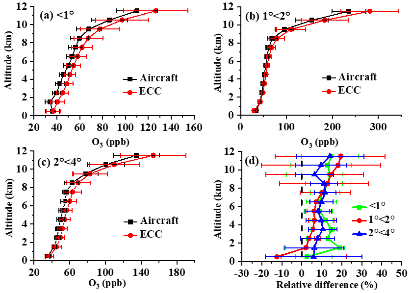
Figure 6 Annual mean vertical profiles of tropospheric O₃ for ECC ozonesonde and aircraft observations at station–pair distances (D) of D<1° (a), $\mathrm{1}\mathit{°}<D<\mathrm{2}\mathit{°}$ (b), and $\mathrm{2}\mathit{°}<D<\mathrm{4}\mathit{°}$ (c). The relative differences for these three categories are shown in panel (d), where the dashed black line represents the zero line.

3.3 Dependence of relative biases on station–airport distances

A major concern when comparing IAGOS and ozonesonde observations is that the stations and airports are not generally co-located, and even when they are close, the flight paths taken by balloons and aircraft are quite different. Figure 6 compares the average vertical distributions of tropospheric O₃ observed at different station–airport distances by ECC sondes and IAGOS. Note that we continue to separate sonde station data by type – only ECC data are used here. Sonde–aircraft pairs have been grouped by station–airport distance (Table 1). The differences in average bias vary only very modestly between the different station–airport distance categories, and these differences are not statistically significant at the 95 % confidence level (Fig. 6d). This, partially owing presumably to the use of mean monthly averages, is encouraging as it provides further evidence that the average bias we have derived is strictly an artefact of instrument differences.

Table 3 The bias, correlation coefficient (R), and RMSE for ECC sonde, Indian-sonde, and aircraft observations at different station–airport distances.

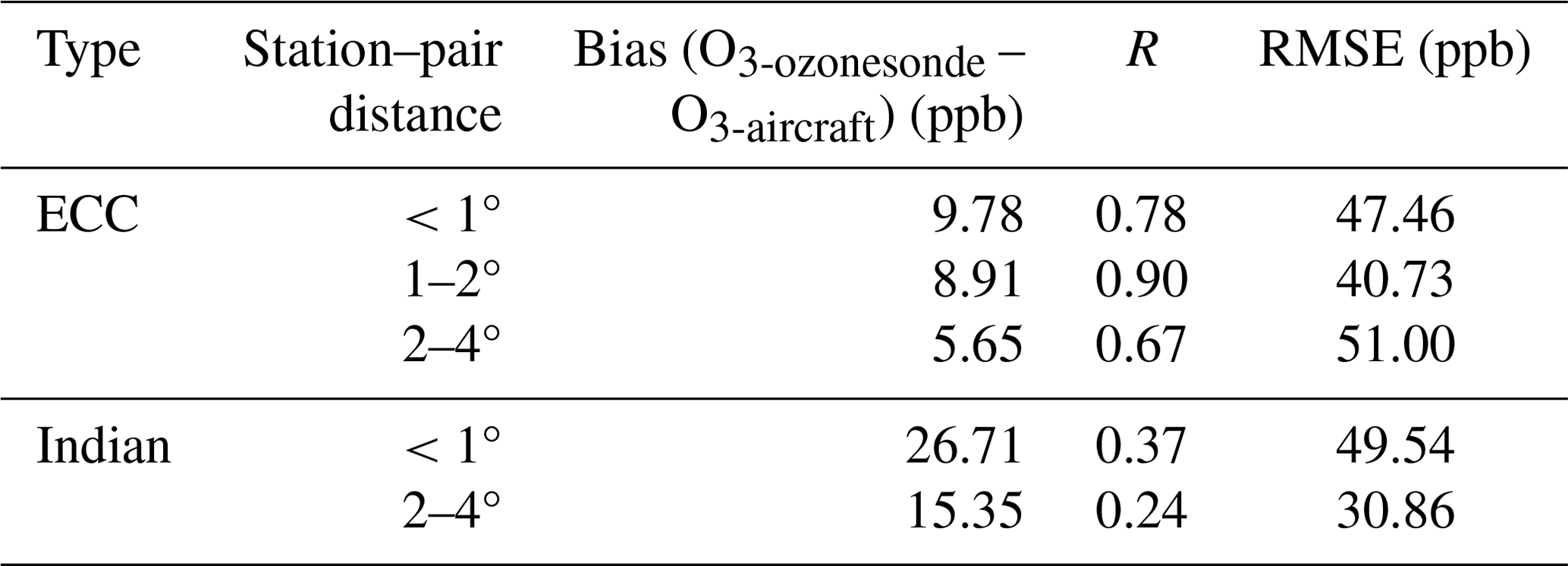
Table 3 indicates that the bias variation between ECC and aircraft observations at different station–airport distances is small, ranging from 5.7 to 9.8 ppb. Correlations for these groupings are also fairly similar, with R values of 0.8, 0.9, and 0.7.

Compared with ECC sondes, the consistency between Indian-sonde and aircraft observations is poor at all station–airport distances, exhibiting much larger biases and poor correlations, with R values ranging from 0.2 to 0.4. Nevertheless, Fig. S5 in the Supplement shows that the profiles of average differences are quite similar for station–airport distances <1° and distances of 2–4° (Fig. S5c).

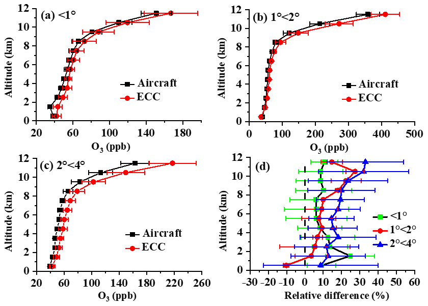
Figure 7 Seasonal mean vertical profiles of tropospheric O₃ in spring for ECC ozonesonde and aircraft observations at station–pair distances (D) of D<1° (a), $\mathrm{1}\mathit{°}<D<\mathrm{2}\mathit{°}$ (b), and $\mathrm{2}\mathit{°}<D<\mathrm{4}\mathit{°}$ (c). The relative differences for these three categories are shown in panel (d), where the dashed black line represents the zero line.

Figures 7 and S6–S8 examine possible seasonal variations in the differences at different station–airport distances for ECC sondes. The mean differences for the different station–airport distance categories are larger than those for the annual averages (Fig. 6), but in general, these differences are not statistically different at the 95 % confidence level (Figs. 7d and S6d–S8d).

3.4 Comparison of ozonesonde relative biases under operational conditions using IAGOS observations as a transfer standard

The foregoing discussion demonstrates that, consistent with previous work, there is a fairly constant relative bias between IAGOS and sondes, with considerable dependence on sonde type, as expected from previous sonde intercomparisons, such as JOSIE 1996. Although uncertainties are sizeable due to the relatively sparse nature of the available data, we find consistent differences at all sites, with little dependence on season or on station–airport separation, as well as little regional dependence (not shown). Notwithstanding this overall sonde–IAGOS bias, we can use these station–airport comparisons to derive relative biases for the different sonde types in use in the global network.

This does not assume that the aircraft data are unbiased. The true value of the O₃ profile (or even its average) remains unknown, as do the absolute biases of the sondes and IAGOS. However, it does assume the following:

1. It assumes that the measurement errors are random and normally distributed.

2. It also assumes that there is one constant bias for each measurement type (i.e. if, for example, the Indian sonde changed over the period of comparison, or if the IAGOS instruments had different biases, there would be additional error not accounted for in our uncertainty estimate).

3. Finally, it assumes that the measurement biases are not dependent on geographic location or variability in the O₃ profile. This does not assume that the average O₃ profile is the same; rather, it indicates that the instruments respond in the same way.

Table 4 Comparison of the different sonde types with IAGOS (average ±2 times the standard error (SE)). “Indian/ECC” refers to (Indian/IAGOS)/(ECC/IAGOS), “Brewer–Mast/ECC” refers to (Brewer–Mast/IAGOS)/(ECC/IAGOS), and “Carbon–iodine/ECC” refers to (Carbon–iodine/IAGOS)/(ECC/IAGOS).

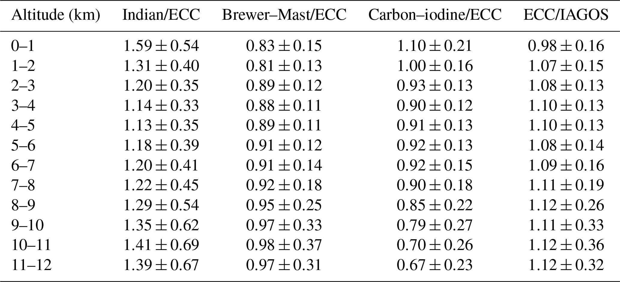
With these assumptions, we can use the results of Fig. 2 to estimate the relative biases of each sonde type in relation to one another. The uncertainty in the comparisons will be the quadratic sum of the uncertainties in the two IAGOS–sonde comparisons. The results are shown in Table 4. This intercomparison of the different sonde types has an important advantage: it compares ozonesonde relative biases under operational conditions as it compares data that are actually in the databases (e.g. the WOUDC database). It also fills a gap as the last international WMO intercomparison involving all four sonde types was JOSIE 1996. These results are broadly consistent with those from JOSIE 1996 (Table 8 and Fig. 11 in Smit and Kley, 1998).

In fact, the types of ozonesondes have changed during long-term observations at some stations (e.g. Uccle and Payerne). De Backer et al. (1998) showed that with the use of an appropriate correction procedure that accounts for the loss of pump efficiency with decreasing pressure and temperature, it is possible to reduce the mean difference between O₃ profiles obtained with both types of sondes to below 3 %, which is statistically insignificant over nearly the entire operational altitude range (from the ground to 32 km altitude). Stübi et al. (2008) also found that the O₃ difference between the Brewer–Mast and ECC ozonesonde data shows good agreement between the two sonde types and that the profile of the O₃ difference is limited to ±5 % (±0.3 mPa) from the ground to 32 km altitude. The results for Brewer–Mast sondes, shown in Table 4, should also be applicable to older Payerne and Uccle records and are generally consistent with these findings and with those from older Canadian records (Tarasick et al., 2002, 2016).

The results in Table 4 will be quite valuable for addressing the problem of relative biases when merging ozonesonde data into global climatologies (e.g. McPeters et al., 2007; McPeters and Labow, 2012; Bodeker et al., 2013; Liu et al., 2013; Hassler et al., 2018).

4 Conclusions

The vertical distributions of tropospheric O₃ observed by ozonesondes and IAGOS sensors from 1995 to 2021 are compared at 23 pairs of sites between about 30° S and 55° N. Overall, ECC, Brewer–Mast, and carbon–iodine sondes agree reasonably well with aircraft observations, with average biases of 2.58, −0.28, and 0.67 ppb and correlation coefficients of 0.72, 0.82, and 0.66, respectively. The agreement between the aircraft and Indian-sonde observations is poor, with an average bias of 15.32 ppb and an R value of 0.44. Ozonesondes and aircraft observations exhibit smaller R values in the middle troposphere but a larger bias and RMSE in the upper troposphere. The bias and RMSE relative to the aircraft observations obtained at different altitudes for the ECC, carbon–iodine, and Brewer–Mast sondes are lower than those for the Indian sondes.

Notwithstanding this general agreement, all sonde types show significant average biases with respect to IAGOS. The O₃ concentration observed by ECC sondes is, on average, higher by 5 %–10 % than that observed by IAGOS, and the relative bias increases modestly with altitude. Seasonal variations in the relative bias are generally not statistically significant. The distance between the station and airport, when within 4° (latitude and longitude), also has little effect on the comparison results. When the ECC station pairs are grouped by station–airport distances of <1° (latitude and longitude), 1–2°, and 2–4°, biases with respect to IAGOS measurements vary from 5.7 to 9.8 ppb, and correlations vary from 0.7 to 0.9.

Thus, the average relative bias observed between the sondes and IAGOS in this study, also noted by previous authors (Zbinden et al., 2013; Staufer et al., 2013, 2014; Tanimoto et al., 2015; Tarasick et al., 2019), is a robust result. Possible reasons for the difference include side reactions that cause sondes to produce excess iodine (Saltzman and Gilbert, 1959) and/or loss of O₃ on the inlet pump, which could cause IAGOS monitors to register low readings at pressures below 800 hPa. The latter was an issue in earlier aircraft O₃ sampling programmes (Schnadt Poberaj et al., 2007; Dias-Lalcaca et al., 1998; Brunner et al., 2001), but Thouret et al. (1998) found this to be negligible for MOZAIC–IAGOS. A recent intercomparison campaign conducted at the World Calibration Centre for Ozone Sondes (WCCOS) in Jülich in June 2023 indicated that the pumps do not greatly influence the IAGOS ozone measurements between 1000 and 200 hPa. The IAGOS-CORE Package1 O₃ measurements (with pressurization pumps) and IAGOS-CARIBIC O₃ measurements differ by less than 2 %, and the WCCOS reference UV-photometer measurements are usually higher by 1 %–2 % (up to a maximum of 5 %) compared to both IAGOS instruments (Blot et al., 2021; Nédélec et al., 2015; Thouret et al., 2022). IAGOS-CARIBIC does not have a pressurization system, which is why the good comparison between both IAGOS systems means a lot.

However, as noted by Saltzman and Gilbert (1959), the differences in stoichiometry found at different pH values imply that the chemistry of the reaction of O₃ with KI is complex, involving reactions that cause a loss of iodine as well as reactions other than the principal one that produce additional iodine. Several authors have noted the existence of slow side reactions involving the phosphate buffer, with a time constant of about 20 minutes, which may also increase the stoichiometry from 1.0 (Tarasick et al., 2021; Smit et al., 2024). Furthermore, evaporation causes the concentration of the sensing solution to increase, which can further enhance the stoichiometry by concentrating the phosphate buffer and, to a lesser degree, by increasing the concentration of KI itself (Johnson et al., 2002). These factors may contribute to the average relative bias observed between the sondes and IAGOS in this study.

This result implies that care must be taken when merging ozonesonde and IAGOS measurement datasets. While the aircraft and sonde measurements are often complementary, filling in important spatial gaps that would otherwise exist if only one type were used, the records do not typically cover the same period, which means merging can introduce spurious jumps if relative biases are not taken into account.

The importance of O₃ in the troposphere as both an air pollutant and a greenhouse gas – and therefore the importance of accurate measurements of its temporal and spatial distribution – implies that resolving the causes of this bias is essential. Thus, further research involving more direct comparisons of IAGOS instrumentation and ozonesondes, e.g. in the WCCOS chamber, is strongly recommended.

These results are also useful for evaluating the relative biases of the different sonde types in the troposphere, using the aircraft as a transfer standard. This intercomparison of the different sonde types has the advantage of comparing ozonesonde relative biases under operational conditions – that is, it uses data that are actually in the databases (e.g. the WOUDC database). These results will be invaluable for addressing relative biases when merging ozonesonde data into global climatologies (e.g. Bodeker et al., 2013; Hassler et al., 2018; Liu et al., 2013; McPeters et al., 2007; McPeters and Labow, 2012).