Observational and model evidence for a prominent stratospheric influence on variability in tropospheric nitrous oxide

The literature presents different views on how the stratosphere influences variability in surface nitrous oxide (N₂O) and on whether that influence is outweighed by surface emission changes driven by the El Niño–Southern Oscillation (ENSO). These questions are investigated using a chemistry–climate model with a stratospheric N₂O tracer; surface and aircraft-based N₂O measurements; and indices for ENSO, polar lower stratospheric temperature (PLST), and the stratospheric quasi-biennial oscillation (QBO). The model simulates well-defined seasonal cycles in tropospheric N₂O that are caused mainly by the seasonal descent of N₂O-poor stratospheric air in polar regions with subsequent cross-tropopause transport and mixing. Similar seasonal cycles are identified in recently available N₂O data from aircraft. A correlation analysis between the N₂O atmospheric growth rate (AGR) anomaly in long-term surface monitoring data and the ENSO, PLST, and QBO indices reveals hemispheric differences. In the Northern Hemisphere, the surface N₂O AGR is negatively correlated with winter (January–March) PLST. This correlation is consistent with an influence from the Brewer–Dobson circulation, which brings N₂O-poor air from the middle and upper stratosphere into the lower stratosphere with associated warming due to diabatic descent. In the Southern Hemisphere, the N₂O AGR is better correlated to QBO and ENSO indices. These different hemispheric influences on the N₂O AGR are consistent with known atmospheric dynamics and the complex interaction of the QBO with the Brewer-Dobson circulation. More airborne surveys extending to the tropopause would help elucidate the stratospheric influence on tropospheric N₂O, allowing for better understanding of surface sources.

1 Introduction

Nitrous oxide (N₂O) is a long-lived greenhouse gas with a global warming potential of 273 relative to CO₂ over a 100-year time horizon (Forster et al., 2021). N₂O has an atmospheric lifetime of about 120 years and is destroyed slowly in the stratosphere by both photolysis and oxidation, with a fraction of the oxidation product yielding NO_x, a catalyst of stratospheric ozone destruction (Crutzen, 1974; Ravishankara et al., 2009; Prather et al., 2015). N₂O has abundant natural microbial sources in soil, freshwater, and oceans, which account for the majority of global emissions, although anthropogenic sources are becoming increasingly important (Tian et al., 2020; Canadell et al., 2021).

The atmospheric N₂O concentration has risen from about ∼ 270 ppb in the preindustrial period to 336 ppb by 2022 (MacFarling-Meure et al., 2006; Lan et al., 2022). This rise has been attributed largely to Haber–Bosch industrial nitrogen (N) fixation to produce agricultural fertilizer, which has increased the substrate available to N cycling microbes (Park et al., 2012). Recent evidence suggests that N₂O is increasing at an accelerating rate in the atmosphere, possibly due to a nonlinear response of microbes to increasing N inputs in intensively fertilized agricultural systems (Thompson et al., 2019; Liang et al., 2022).

High-precision measurements of N₂O have revealed interannual variability in its atmospheric growth rate (AGR) and small-amplitude seasonal cycles in the range of 0.4 to 1 ppb (Nevison et al., 2004, 2007, 2011; Jiang et al., 2007; Thompson et al., 2013). Spatial gradients in atmospheric N₂O are also small, e.g., the Northern Hemisphere (NH) minus Southern Hemisphere (SH) difference is approximately 1 ppb (Thompson et al., 2014; Liang et al., 2022). Larger spatial and seasonal signals in atmospheric N₂O have been observed at sites influenced by strong local agricultural or coastal upwelling sources (Lueker et al., 2003; Nevison et al., 2018; Ganesan et al., 2020). However, at sites remote from local sources even variations of 0.2 ppb in estimated background N₂O levels can significantly affect the magnitude of N₂O emissions inferred from atmospheric inversions (Nevison et al., 2018).

A few studies have inferred information about surface biogeochemical sources based on the observed seasonal cycle in atmospheric N₂O at remote monitoring sites. However, these studies have cautioned that the transport of N₂O-poor air from the stratosphere is a major cause of both seasonal and interannual variability in surface N₂O, which complicates the interpretation of surface emission signals (Nevison et al., 2005, 2011, 2012; Thompson et al., 2014; Ray et al., 2020; Ruiz et al., 2021). Other studies have argued that El Niño–Southern Oscillation (ENSO) cycles are the major driver of interannual variability in tropospheric N₂O (Ishijima et al., 2009; Thompson et al., 2013; Canadell et al., 2021) or that ENSO-driven variability can obscure the influence of the stratosphere in some years (Ruiz et al., 2021). ENSO refers to the periodic oscillation between warm (El Niño) and cold (La Niña) phases in sea surface temperature over the eastern tropical Pacific (ETP). During the El Niño phase, the warming and deepening of the thermocline is associated with reduced upwelling in the ETP and drought in South America, which can decrease oceanic and soil N₂O emissions, respectively (McPhaden et al., 1998; Ishijima et al., 2009; Babbin et al., 2015).

Studies of the stratospheric influence on surface N₂O variability have differed with respect to the relative impact on the NH and SH. Ray et al. (2020) found a direct correlation between the stratospheric quasi-biennial oscillation (QBO), lagged by 8–12 months, and the observed surface N₂O AGR, but this was found in the SH only. The QBO is a tropical, stratospheric, and downward-propagating zonal wind variation with an average period of ∼ 28 months that dominates the variability of tropical lower stratospheric meteorology (Baldwin et al., 2001; Butchart, 2014). Ruiz et al. (2021) found a direct correlation between the QBO and N₂O photochemical loss rates in the tropical middle stratosphere but concluded that interannual variability in surface N₂O globally was governed more by changes in the dynamical processes of the lowermost stratosphere. They showed evidence for a coherent influence of cross-tropopause transport on the surface N₂O seasonal cycle in the NH but not the SH.

Nevison et al. (2011) argued that cross-tropopause transport and mixing drives the N₂O seasonal minimum in both hemispheres based on significant correlations between surface N₂O seasonal anomalies and stratospheric indices reflective of the Brewer–Dobson circulation (BDC). The BDC is a planetary-wave-driven, large-scale meridional circulation that transports ozone, greenhouse gases, and other constituents poleward and maintains the thermal structure of the stratosphere (Butchart, 2014; Minganti et al., 2020). As part of this transport, the BDC brings N₂O-poor air from the tropical middle and upper stratosphere into the polar lower stratosphere in the winter hemisphere (Liang et al., 2008, 2009; Nevison et al., 2011).

A better grasp of the controls on tropospheric N₂O variability has important implications for the interpretation of biogeochemical signals in N₂O data. If abiotic factors associated with the downward transport of N₂O-poor air from the stratosphere contribute significantly to variability, they must be disentangled from the data before inferring information about surface biogeochemistry and emissions. Understanding the influence of stratospheric variability on surface N₂O also may provide insight into anomalous changes in the AGR of CFC-11, which has a stratospheric sink similar to that of N₂O (Ray et al., 2020; Ruiz et al., 2021; Lickley et al., 2021).

This paper explores the causes of variability in both the seasonal cycle and the AGR of tropospheric N₂O. It follows up on previous work by Nevison et al. (2011), who inferred a stratospheric influence on surface atmospheric N₂O data based entirely on correlations between interannual variations in stratospheric indices and detrended N₂O anomalies in months surrounding the seasonal N₂O minimum. In the meantime, observed altitude–latitude cross sections have become available from aircraft surveys that span a full seasonal cycle. In addition, advances in model development allow for explicit simulation of stratospheric N₂O tracers (Ruiz et al., 2021; Liang et al., 2022).

This study uses the NASA Goddard GEOS-5 Chemistry-Climate Model (GEOSCCM), which includes a tagged stratospheric N₂O tracer that is transported individually in the model and can be distinguished from tropospheric tracers of fresh surface emissions (Liang et al., 2022). The study also examines atmospheric N₂O data collected in the NH by the National Oceanic Atmospheric Administration (NOAA) during routine aircraft monitoring, as well as N₂O data measured by recent global airborne surveys spanning both hemispheres. Finally, it performs an updated correlation analysis of surface N₂O anomalies from ground-based NOAA sites against ENSO and QBO indices and polar lower stratospheric temperature (PLST), which is used as a tracer for the BDC, with the assumption that significant correlations provide support (although not proof) for causation.

The paper is organized as follows. Section 2 describes the data and methods used. Section 3 presents the results, beginning in Sect. 3.1 with an examination of climatological mean seasonal cycles and latitude–altitude cross sections of N₂O from GEOSCCM and aircraft data. Section 3.2 examines correlations between variability in the N₂O AGR from NOAA long-term surface monitoring data, PLST, and indices of QBO and ENSO. Section 3.3 examines correlations between PLST and variability in monthly N₂O anomalies near the month of seasonal minimum. Section 3.2 and 3.3 include parallel correlation analyses of variability in GEOSCCM N₂O sampled at NOAA surface sites and GEOSCCM-based QBO and PLST indices. Section 4 interprets and discusses the results. Section 5 finishes with a summary and future outlook.

2 Methods

2.1 GEOSCCM with tagged stratospheric tracers

GEOSCCM was used to simulate atmospheric N₂O with geographically resolved surface emissions from soil, ocean, and anthropogenic sources and full stratospheric chemistry with stratospheric N₂O destruction due to photolysis and O(¹D) oxidation (Nielsen et al., 2017; Liang et al., 2022). GEOSCCM has been evaluated extensively in multi-model assessments and shown to accurately represent the mean atmospheric circulation, the interhemispheric exchange rate, the mean age of air in the tropical and polar stratosphere, and the mean atmospheric lifetime of N₂O (Liang et al., 2022, and references therein). For the current study, GEOSCCM was run at 1° × 1° resolution with 72 vertical layers from the surface to 0.01 hPa. In addition to the standard total N₂O tracer, four additional N₂O tracers were included to track the following items: (1) aged air from the stratosphere (N2O_ST) and (2) soil, (3) ocean, and (4) anthropogenic sources freshly emitted in the troposphere. Following the approach of Liang et al. (2008), the tropospheric tracers become the stratospheric tracer, N2O_ST, when they are transported across the tropopause and retain that identity even when N2O_ST re-enters the troposphere, thereby providing a model estimate of the stratospheric influence on tropospheric N₂O.

The full GEOSCCM simulation spanned 1980–2019, but this study focuses on the final 20 years from 2000–2019 for the correlation analysis between model surface N₂O anomalies and QBO and PLST. As described in detail in Liang et al. (2022), the GEOSCCM N₂O lifetime decreased slightly after 2000 (from 119±2 years in the 1990s down to 116±2 years in the 2010s), and model emissions were optimized to account for the observed change in the atmospheric N₂O growth rate. GEOSCCM temperature and QBO do not necessarily correspond to observations since both are internally generated by the GEOS general circulation model, which is free running rather than forced by a reanalysis meteorology. GEOSCCM PLST and QBO were computed in the same way as the observed indices, as described below in Sect. 2.4.1 and 2.4.2, respectively. The GEOSCCM N₂O fields were saved as monthly means and were detrended and converted to anomalies by subtracting a deseasonalized fit to the model time series sampled at Mauna Loa (MLO). The N₂O time series at MLO is a good proxy for the global N₂O trend, and thus its subtraction provides a convenient, single-station approach for calculating anomalies of the N₂O mixing ratio for contour plots.

2.2 N₂O data

2.2.1 Surface N₂O from NOAA long-term monitoring sites

Surface atmospheric N₂O data were obtained from the NOAA Global Monitoring Laboratory (GML) for comparison to GEOSCCM output. NOAA has two programs that measure N₂O, Halocarbons and other Atmospheric Trace Species (HATS, Hall et al., 2007) and the Carbon Cycle Greenhouse Gases group (CCGG, Lan et al., 2022). HATS provides in situ data measured every ∼ 60 min using the Chromatograph for Atmospheric Trace Species (CATS) instruments at five baseline sites (Utqiaġvik, Alaska; Niwot Ridge, Colorado; Mauna Loa, Hawaii; Cape Grim, Tasmania; and South Pole, Antarctica). CCGG maintains a flask air sampling network at ∼55 widely distributed surface sampling sites, in which duplicate samples are collected roughly weekly and shipped to Boulder, Colorado, for analysis by gas chromatography (GC) with electron capture detection (ECD) and by a tunable infrared laser direct absorption spectroscopy (TILDAS) after August 2019. The instruments are calibrated with a suite of standards on the WMO X2006A scale maintained by NOAA GML (Hall et al., 2007). Uncertainties in the measurements (68 % confidence interval) range from 0.26 to 0.43 ppb with GC-ECD and ∼ 0.16 ppb with TILDAS. The mean uncertainties in CATS GC data are 0.2 to 1.2 ppb (68 % confidence interval) over most of the 2000s, with an increase in recent years as the instruments age.

This study used the NOAA combined HATS/CCGG N₂O product from 1998–2021, which is based on monthly medians from the CATS in situ program (at the five HATS baseline sites) and monthly means from the CCGG flask program at a selected subset of 12 of the ∼ 55 total sites (https://doi.org/10.15138/GMZ7-2Q16; Hall et al., 2007). All of the NOAA sites considered in this study are long-standing remote sites situated away from strong local anthropogenic sources. They include Alert, Canada; Summit, Greenland; Mace Head, Ireland; Trinidad Head, California, Cape Kumukahi, Hawaii, Cape Matatula, Samoa; Palmer Station, Antarctica; and the five HATS baseline sites (at which CCGG also makes overlapping flask measurements). In addition to these 12 individual sites, global, NH and SH means are estimated from the latitude-binned and mass-weighted means of the combined monthly means for the 12 sites (Hall et al., 2011). The combined monthly data are first aggregated at the measurement program level for each sampling location. At sites where both HATS and CCGG measure, a weighted mean is calculated based on the programs' monthly uncertainties.

2.2.2 NOAA empirical background for atmospheric N₂O

The NOAA empirical background is a four-dimensional (4-D) field, constructed from NOAA surface and aircraft N₂O data, which is used in North American regional inversions to represent the background concentration of atmospheric N₂O prior to the influence of continental surface fluxes (Nevison et al., 2018). The 4-D field is defined daily over North America from 500–7500 m every 1000 m, from 170°–50° W every 10° longitude, and from 20–70° N every 5° latitude (or, prior to 2017, from 20-80° N every 10° latitude). For this study, a deseasonalized fit to the NOAA time series at Mauna Loa was used to detrend and remove the mean value (centered in the mid troposphere) of the empirical background data, thus allowing them to be collapsed into a single climatological year and presented as anomalies. The climatology encompassed 1 January 2005–31 December 2013, a period when atmospheric N₂O was increasing by about 0.9 ppb yr⁻¹.

2.2.3 N₂O data from global airborne surveys

Atmospheric N₂O measurements were made in situ with the Harvard/Aerodyne Quantum Cascade Laser Spectrometer (QCLS) on three different aircraft campaigns designed to study the atmospheric profiles of greenhouse and related gases (Wofsy et al., 2011; Stephens et al., 2018). QCLS N₂O data are retrieved at 1 Hz with 1 s precision of 0.09 ppb and reproducibility with respect to the WMO N₂O scale of 0.2 ppb (Kort et al., 2011; Santoni et al., 2014) on the NOAA-2006 scale (Hall et al., 2007). The first of the campaigns, the High-performance Instrumented Airborne Platform for Environmental Research (HIAPER) Pole to Pole Observations (HIPPO) project, consisted of five roughly month-long sets of flights centered over the central Pacific Ocean extending from the surface to the upper troposphere–lower stratosphere and nearly pole to pole (Wofsy et al., 2011). The flights were timed between January 2009 and November 2011 to create a climatological seasonal cycle. The second campaign, ${\mathrm{O}}_{\mathrm{2}}/{\mathrm{N}}_{\mathrm{2}}$ Ratio and CO₂ Airborne Southern Ocean (ORCAS), took place in January–February 2016 and focused on the Southern Ocean south of ∼35° S (Stephens et al., 2018). Most recently, the Atmospheric Tomography Mission (ATom) campaign extended nearly pole to pole over both the Pacific and Atlantic oceans. ATom consisted of four deployments over 3 years, with each deployment approximately 1 month long (Thompson et al., 2022). QCLS N₂O was measured during the second through fourth ATom deployments in January/February 2017, September/October 2017, and April/May 2018, respectively, but N₂O measurements are not available from the first ATom deployment in July/August 2016 due to technical problems (Gonzalez et al., 2021). For all figures presented below using QCLS N₂O, the flight track data were interpolated onto a 5° latitude by 50 hPa grid using the akima package in R (Akima, 1978). In addition, a deseasonalized fit to the NOAA time series at Mauna Loa was subtracted from all data, allowing them to be collapsed into a climatological year and expressed as anomalies.

2.3 Mean seasonal cycles and interannual variability in surface N₂O

Mean seasonal cycles for NOAA surface N₂O observations and GEOSCCM N₂O tracers were estimated using a bootstrapping method in which 20 % of the time series was randomly removed and the remaining 80 % was fit to a third-order polynomial plus first four harmonics. These steps were repeated over 500 iterations to estimate the range of uncertainty in the harmonic components of the fit.

Interannual variability in the atmospheric growth rate of N₂O in the NOAA surface NH, SH, and global time series was calculated by first removing the seasonal cycle from the monthly mean time series by computing a 12-month running average,

$$\begin{array}{}\text{(1)}& X_i=(C_{i-\mathrm{6}}+\mathrm{2}\sum _{k=i-\mathrm{5}}^{i+\mathrm{5}}{C}_k+C_{i+\mathrm{6}})/\mathrm{24},\end{array}$$

where C is the original monthly mean time series and X is the deseasonalized time series. The slope of the deseasonalized time series then was computed as a central difference,

$$\begin{array}{}\text{(2)}& S_i=\mathrm{12}{\displaystyle \frac{x_{i+\mathrm{1}}-x_{i-\mathrm{1}}}{\mathrm{2}}},\end{array}$$

where S is the centrally differenced slope and the scalar 12 converts S from units of parts per billion per month to parts per billion per year. To account for the increasing growth rate of atmospheric N₂O, the absolute slopes S were converted to atmospheric growth rate anomalies by removing an optimal (increasing) linear fit determined by recursive least-squares regression.

Interannual anomalies in the magnitude of the seasonal minimum were calculated by detrending the raw monthly mean N₂O data with a third-order polynomial, after which a climatological seasonal cycle was constructed by taking the average of the detrended data for all Januaries, Februaries, etc. This climatological annual cycle was subtracted from the original raw data to produce a deseasonalized (but not detrended) time series. A running 12-month annual mean of this curve was then computed as in Eq. (1) but where C is now the deseasonalized time series rather than the original monthly mean time series. This analysis focused on mid- and high-latitude sites in the NOAA dataset. At stations with gaps in the monthly data, the original third-order polynomial fit was used as a placeholder in the running mean. The running mean was subtracted from the deseasonalized curve to remove the secular trend and other low-frequency variability, thus isolating the residual monthly anomalies.

2.4 Proxies and indices for the correlation analysis

The computation of N₂O AGR anomalies from Sect. 2.3 created a set of monthly resolved time series for the SH, NH, and global means. These were plotted against various proxies and indices for stratospheric influences and ENSO. In addition, the high-frequency residuals from Sect. 2.3 at various mid- and high-latitude sites were sorted by month, and selected months were plotted against PLST as described below in Sect. 2.4.1. The PLST proxy involves a single value for each year, such that correlation coefficients and p values were computed based on the number of years N with data. For the ENSO and QBO indices, the correlation statistics were computed based on the reduced, effective N (N_eff) number of monthly data points after accounting for the autocorrelation that is introduced by the 12-month running mean used to compute the N₂O AGR (see Supplement Sect. S1 for more details.)

2.4.1 Polar lower stratospheric temperature (PLST) as proxy for the Brewer–Dobson circulation

Mean polar (60°–90°) lower stratospheric temperature at 100 hPa in January–March (winter) in the NH and September–November (spring) in the SH was computed from the Modern-Era Retrospective Analysis for Research Applications, Version 2 (MERRA-2), reanalyses (Gelaro et al., 2017). The mean PLST in each hemisphere was treated as a proxy for the integrated strength of the BDC, which brings N₂O-poor air from the middle to upper tropical stratosphere into the polar winter lower stratosphere through diabatic descent. PLST represents the cumulative effect of descent throughout fall and winter, with warmer PLST corresponding to stronger descent (Holton, 2004; Nevison et al., 2007, 2011). Winter months (January–March) were averaged in the NH and spring months (September–November) in the SH to account for the later seasonal breakup of the Antarctic polar vortex compared to the Arctic polar vortex (Nevison et al., 2011). For the monthly analysis, the PLST proxy was regressed against the monthly N₂O anomaly in each of the subsequent months leading up to and encompassing the seasonal minimum in tropospheric N₂O, which occurs in summer in the NH and autumn in the SH. For the AGR analysis, the mean N₂O AGR anomaly was averaged over 12 months (considering a range of start and end months) for regression against PLST.

2.4.2 Quasi-biennial oscillation (QBO)

The QBO was quantified using monthly mean stratospheric zonal wind values in meters per second derived from twice-daily balloon radiosondes conducted by the Meteorological Service Singapore Upper Air Observatory at a station located at 1.34° N, 103.89° E (https://acd-ext.gsfc.nasa.gov/Data_services/met/qbo/QBO_Singapore_Uvals_GSFC.txt, last access: 19 May 2020). A positive QBO indicates westerly winds, and a negative QBO indicates easterly winds. A range of altitudes from 10 to 100 mb was considered. Since the QBO index is a monthly mean time series, it can be compared directly to the monthly mean N₂O AGR time series. However, delays are expected between the QBO and its influence on tropospheric N₂O (Strahan et al., 2015; Ray et al., 2020). Therefore, a range of lag times was considered spanning 6–24 months when correlating with the N₂O AGR anomalies to identify the optimal QBO altitude and lag in each hemisphere.

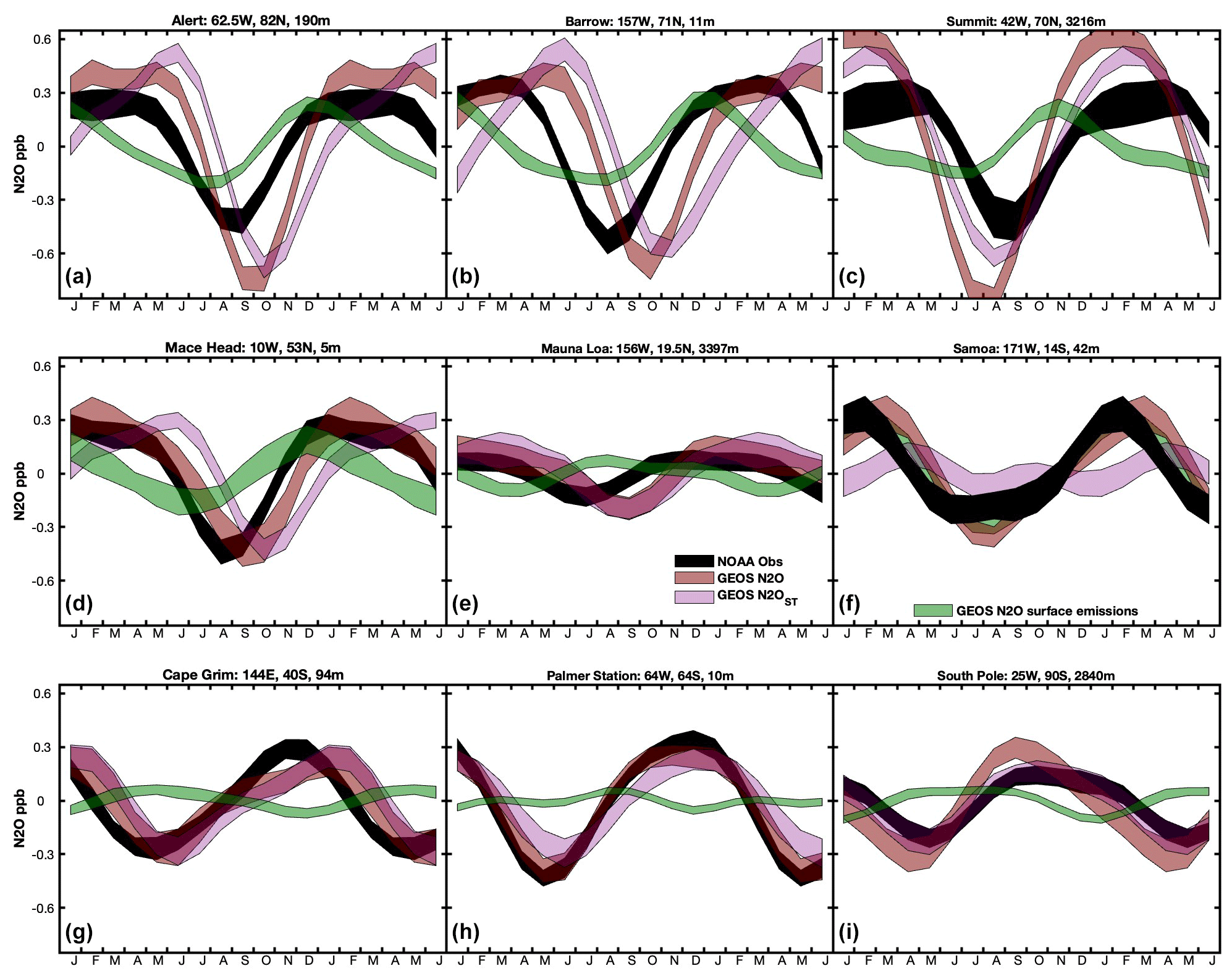
Figure 1 Detrended seasonal cycles in N₂O mixing ratio (ppb) modeled by GEOSCCM and compared to NOAA surface station data at 9 surface sites, with uncertainty estimated using a bootstrap method. Panels (a)–(c) show Alert (Canada), Utqiaġvik (Alaska), and Summit (Greenland). Panels (d)–(f) show Mace Head (Ireland), Mauna Loa (Hawaii), and Cape Matatula (Samoa). Panels (g)–(i) show Cape Grim (Tasmania), Palmer Station (Antarctica), and South Pole (Antarctica). The black line indicates observed N₂O from NOAA. For GEOSCCM, the total N₂O from all forcings is in shown in red, and the stratospheric tracer N₂O_ST is shown in magenta. The green line shows N₂O due to fresh surface emissions, representing the combined net influence of the natural soil, ocean, and anthropogenic atmospheric tracers.

2.4.3 ENSO

ENSO cycles were defined using the Niño 3.4 index, which is based on sea surface temperature anomalies from 5° S to 5° N and 170 to 120° W. The Niño 3.4 index defines an El Niño event as a temperature anomaly of >0.4 °C and a La Ninã event as a temperature anomaly of $<-\mathrm{0.4}$ °C. Monthly Niño 3.4 indices were obtained from https://www.cpc.ncep.noaa.gov/data/indices/sstoi.indices (last access: 14 July 2024). Like the QBO index, Niño 3.4 is a monthly time series that can be compared directly to the monthly mean N₂O AGR time series. In the analysis presented here, a range of lag times in the Niño 3.4 index was considered spanning 0–12 months to identify the optimal lag in each hemisphere.

2.4.4 GEOSCCM correlation analysis

Equations (1) and (2) were applied to GEOSCCM N₂O output sampled at the coordinates of NOAA monitoring sites to create modeled N₂O AGR time series and monthly anomalies, using both total N₂O and N₂O_ST. Similarly, mean winter and spring PLST at 100 hPa was calculated for GEOSCCSM output in the NH and SH, respectively, as described in Sect. 2.4.1, for each model year from 2000–2019. Finally, a GEOSCCM monthly QBO index was calculated at a range of altitudes from 10 to 100 mb by averaging the model zonal wind component in meters per second between 5° S and 5° N over each of the 240 months from 2000–2019. A correlation analysis was performed using the GEOSCCM N₂O AGR and monthly anomaly time series regressed against GEOSCCM PLST and QBO, similar to that described for the observed quantities in Sect. 2.3–2.4. The ENSO correlation analysis was not applied to GEOSCCM output because the model did not attempt to reproduce the impact of ENSO on surface flux variability (Liang et al., 2022).

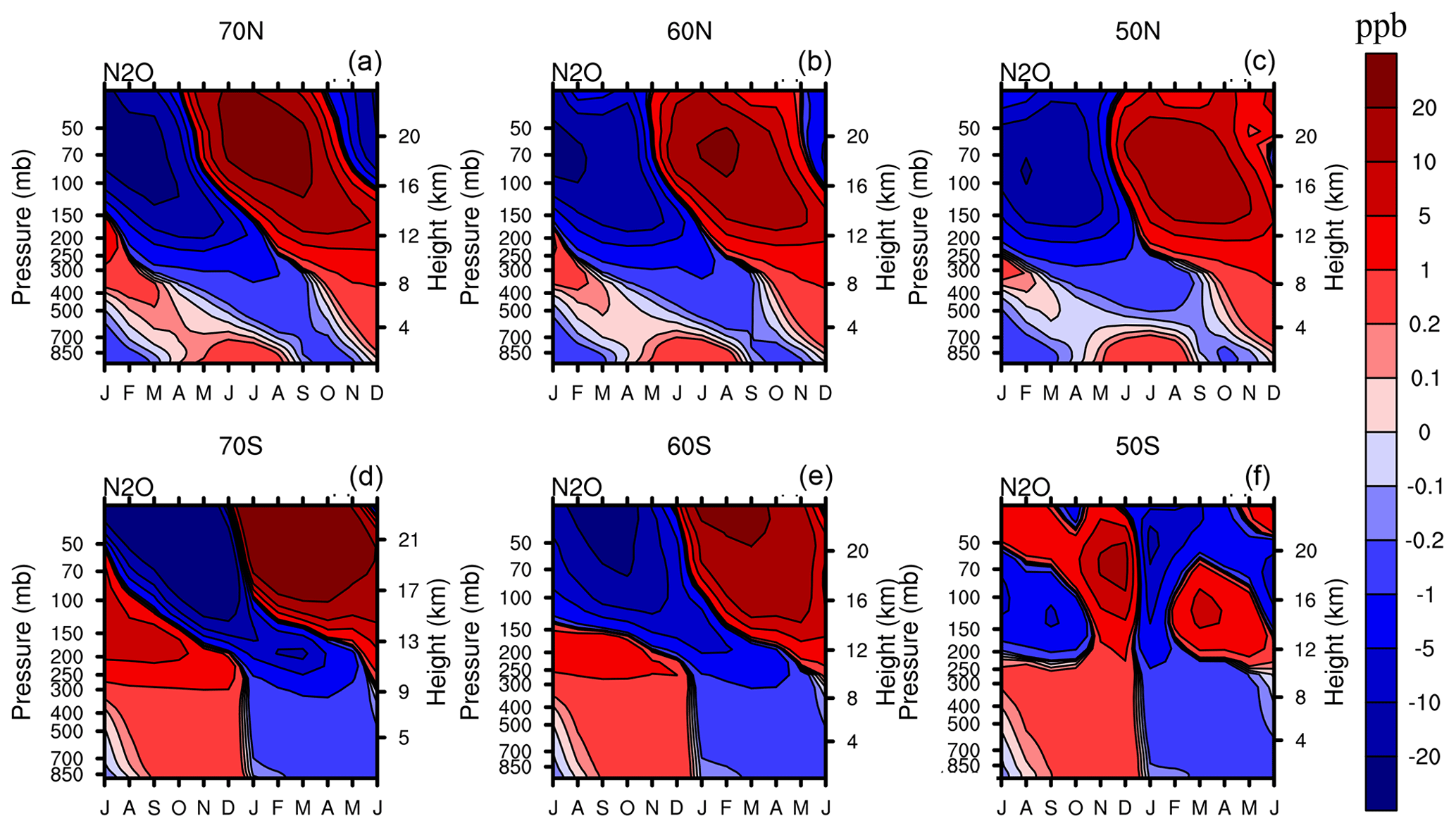
Figure 2 GEOSCCM anomalies of N₂O mixing ratio (ppb) as a function of month and altitude over a mean seasonal cycle, plotted from the surface to 30 hPa in the NH (a–c) and SH (d–f). The columns show, from left to right, 10° latitude bins centered at 70, 60, and 50°. Monthly anomalies are computed by subtracting the annual mean value at each pressure level.

3 Results

3.1 Stratospheric influence on tropospheric N₂O in model and aircraft data

Figure 1 shows that the GEOSCCM N₂O mean seasonal cycle at surface sites is dominated by stratospheric air depleted in N₂O that is transported to the surface, rather than by the influence of surface sources. This dominance holds within the uncertainty of the seasonal cycles, as estimated using a bootstrap method. However, the surface emissions tend to pull the total N₂O seasonal minimum about 1 month earlier than the N2O_ST minimum at most sites. Figure 1 also shows that GEOSCCM captures the mean observed seasonal cycle in N₂O relatively well at sites in the SH but overestimates the amplitude of the cycle at sites in the NH, with a ∼ 1–2-month delay in phasing relative to observations.

Figure 2 provides a two-dimensional view, using zonally averaged altitude–month contour plots at middle and high latitudes in both hemispheres, of how the signal of stratospheric air depleted in N₂O is transmitted to the surface in GEOSCCM. This N₂O-poor air accumulates during winter (starting in ∼ December in the NH and ∼ July in the SH) in the polar stratosphere and descends vertically and crosses into the troposphere in spring (March–April) in the NH and early summer (January–February) in the SH. The SH latitude panels in Fig. 2 are plotted with a 6-month shift to help visualize the later seasonal phasing of the stratospheric influence in the SH relative to the NH. After crossing into the troposphere, the N₂O-poor air continues to move downward and also mixes equatorward from approximately January to May at SH middle to high latitudes and April to October at NH middle to high latitudes (Liang et al., 2009, 2022). Due to lags in downward propagation and mixing, the modeled surface minimum in the lower troposphere does not occur until late summer to early autumn in both hemispheres (Figs. 1 and 2). Figure S1 in the Supplement shows a three-dimensional view of this process in a series of 12 monthly altitude–latitude plots.

Figure 3 shows that the NOAA N₂O empirical background, when organized as a series of zonally averaged altitude–month contour plots at NH latitudes, has features similar to those simulated by GEOSCCM. Both model and observations show a signal of N₂O depletion beginning in early spring in the upper troposphere that propagates down to the surface. In both model and observations, the signal is strongest at high latitudes and weakens substantially moving equatorward. However, the NOAA data suggest a faster, more direct downward propagation of the stratospheric signal, which arrives at the surface in August–September, compared to September–October in GEOSCCM. As a result, the phasing of the GEOSCCM surface minimum is delayed ∼ 1–2 months relative to the NOAA empirical background, consistent with the comparison to NOAA surface monitoring data in Fig. 1.

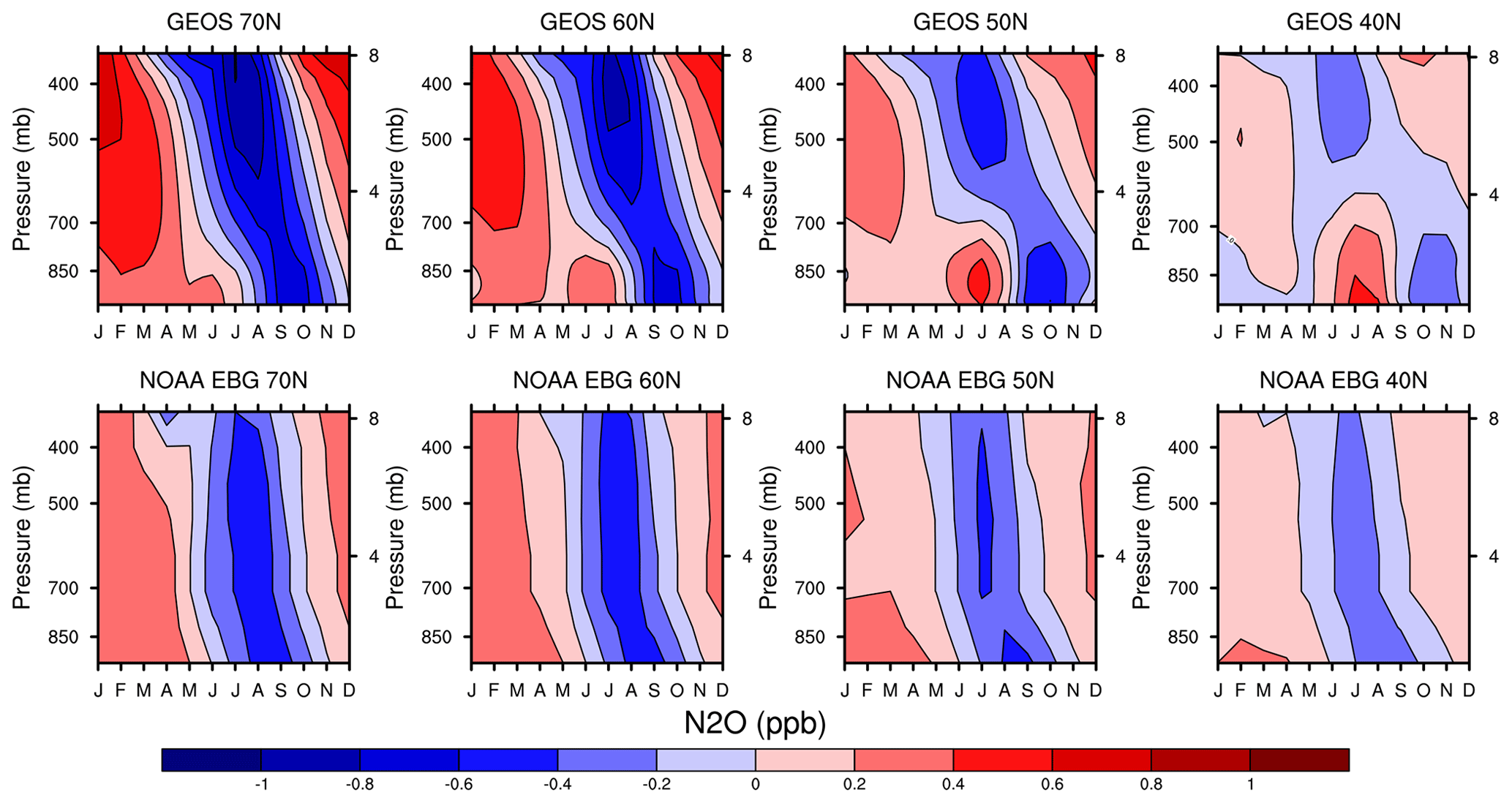
Figure 3 Anomalies of N₂O mixing ratio (ppb) as a function of month and altitude over a mean seasonal cycle, plotted from the surface to 8 km (∼ 330 hPa) in the NH for GEOSCCM (top row) and the NOAA empirical background (bottom row). The columns show, from left to right, 10° latitude bins centered at 70, 60, 50, and 40° N. Monthly anomalies are computed by subtracting the annual mean value at each pressure level.

The positive anomalies in Fig. 3 also differ between model and observations, with surface features centered on July at 40–50° N in GEOSCCM, which uses a summer-dominant soil source (Liang et al., 2022), while the NOAA empirical background shows positive surface anomalies in late winter and spring, likely reflecting North American agricultural sources (Nevison et al., 2018). At 60 and 70° N, the stronger contrast between positive and negative anomalies throughout the atmospheric column in GEOSCCM compared to NOAA reflects the model's larger seasonal cycle, as seen also in Fig. 1.

Figure 4 provides a further perspective on the signal of N₂O-poor stratospheric air in the NOAA empirical background. When viewed as a 12-month sequence of altitude–latitude contours in the NH, the signal originates at northern polar latitudes in the upper troposphere in late winter and early spring and descends and mixes equatorward, with a peak surface influence around July–September at middle to high latitudes in the NH that overshadows any surface source signal. By late fall and winter, the signal has dissipated at the surface but is forming again in the upper troposphere.

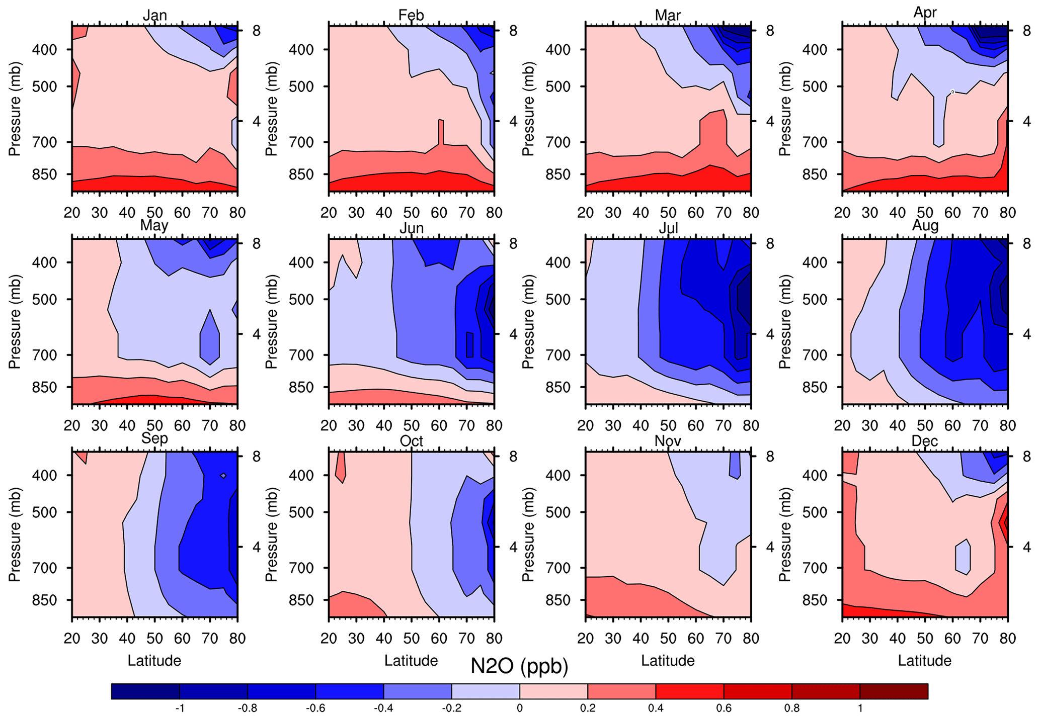
Figure 4 Anomalies of N₂O mixing ratio (ppb) in the NH from the NOAA empirical background, plotted in a monthly sequence of altitude vs. latitude plots extending from the surface up to 8 km (∼330 hPa) and from 20–80° N.

QCLS N₂O data from airborne surveys extend up to 14 km and thus provide a broader perspective with respect to altitude of the stratospheric influence on tropospheric N₂O. Of the three available airborne surveys (HIPPO, ORCAS, and ATom), HIPPO provides the most complete N₂O time series across all seasons. In Fig. 5, the southbound transects from the five HIPPO deployments are detrended and arranged chronologically as altitude–latitude contour plots over an annual mean cycle. These plots form a sequence with a similar movement of N₂O-poor stratospheric air from upper levels down to the surface as seen in GEOSCCM and the NOAA empirical boundary data. This progression is most readily seen in the NH in Fig. 5, in which N₂O-poor air in the polar lower stratosphere has crossed the tropopause by March. By June it has descended into the middle troposphere and started moving equatorward, reaching its maximum influence at the surface in August. By November, the stratospheric signal is no longer visible at the surface following tropospheric mixing and dilution. This seasonal progression is also evident in a fuller dataset that also includes the ATom and northbound HIPPO transects collapsed into a climatological cycle (Fig. S2 in the Supplement)

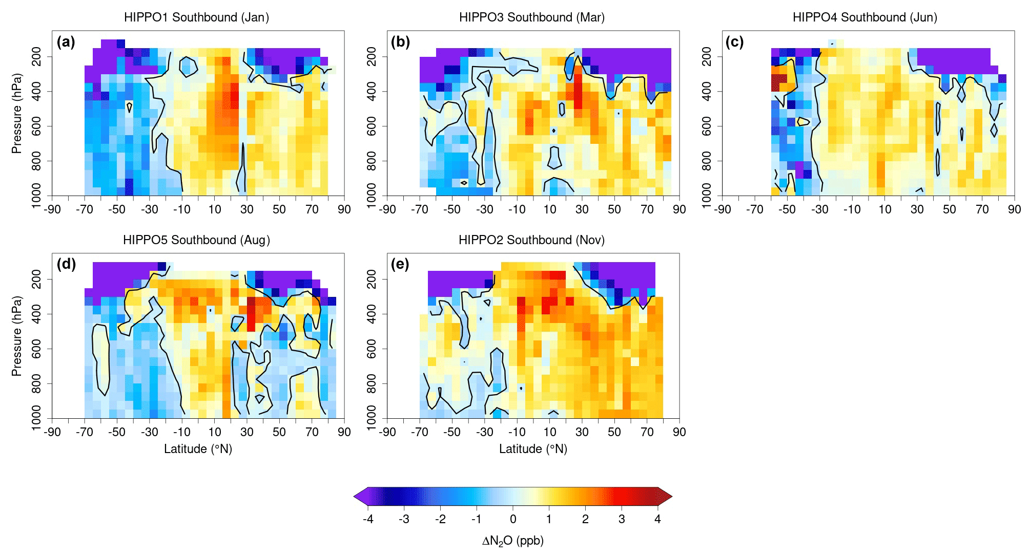
Figure 5 Sequence of five HIPPO pressure–latitude contours of anomalies of N₂O mixing ratio (ppb) arranged to form an annual sequence in January, March, June, August, and November (a–e). Each panel represents a north-to-south transect across latitude with vertical profiling from the surface to 14 km.

3.2 Correlation analysis of the surface N₂O atmospheric growth rate (AGR)

In this section NOAA surface N₂O AGR anomalies from 1998–2020 are plotted against polar lower stratospheric temperature (PLST) and QBO and ENSO indices, with varying lag times as described in Sect. 2. The analysis focuses on the NOAA global, NH, and SH mean products, with the assumption that a significant correlation between the interannual variability in the N₂O AGR and one or more of the indices can be interpreted to support a causal influence on the N₂O AGR. However, correlation does not prove causation and cannot distinguish possible confounding effects, such as the influence of ENSO on both interhemispheric transport and surface sources. A similar correlation analysis is performed for the GEOSCCM N₂O AGR and the model's internally generated QBO and PLST fields, with the assumption that similarities between modeled and observed correlations may also support a causal influence.

Figure 6, which presents correlations between the SH surface N₂O AGR and the QBO and PLST indices, first for NOAA observations and next for GEOSCCM output, shows that the QBO is positively correlated to the NOAA N₂O AGR. The optimal correlation (R=0.55, p<0.01) occurs for QBO in the upper stratosphere at 20 hPa with a time shift of about 18 (17–19) months relative to the N₂O time series. In contrast, spring PLST is not significantly correlated to the NOAA surface N₂O AGR in the SH (Fig. 6b). In Fig. 6c, the correlation between GEOSCCM QBO and the SH N₂O AGR is weak (R=0.24, p>0.10) but also positive in sign in the upper stratosphere with an optimal shift in the GEOSCCM QBO of about 19 months, similar to that found for NOAA. In Fig. 6d, GEOSCCM PLST is significantly anticorrelated with the N₂O AGR averaged over a range of different 12-month intervals, with the highest correlation ($R=-\mathrm{0.61}$, p=0.01) over the 12-month interval from May–April.

Figure 7, which presents the corresponding correlations for the NH surface N₂O AGR, shows that, in contrast to the SH, the NOAA NH N₂O AGR is correlated only weakly to the QBO index at all altitudes and with a negative sign. The highest correlation in the NH occurs for 50 hPa QBO ($R=-\mathrm{0.21}$, p>0.1) with a 10–14-month lag (Fig. 7a). However, the NOAA NH N₂O AGR is anticorrelated significantly to winter PLST ($R=-\mathrm{0.69}$, p<0.001), with an optimal correlation for the 12-month period from July–June encompassing the January–March PLST average (Fig. 7b). GEOSCCM predicts an anticorrelation ($R=-\mathrm{0.47}$, p<0.05) between the QBO and the NH N₂O AGR, which is optimal around 50 hPa with 10–14-month QBO lag, similar to NOAA (Fig. 7c), and also predicts an anticorrelation between PLST and NH N₂O AGR ($R=-\mathrm{0.55}$, p=0.02) (Fig. 7d).

Figure 8, which presents correlations between the Niño 3.4 index and the NOAA surface N₂O AGR, shows that the two are significantly anticorrelated ($R\sim -\mathrm{0.4}$, p<0.05) for both the global and SH N₂O AGR, with little or no monthly lag in the index. In the NH, the anticorrelation is weaker ($R=-\mathrm{0.26}$, p>0.10) with an optimal lag of 7 months in the Niño 3.4 index relative to the N₂O AGR (Fig. 8).

3.3 Correlation analysis of N₂O monthly anomalies

The N₂O monthly anomaly correlation analysis is focused solely on PLST, which has one unique value each year that can be plotted against the corresponding N₂O anomaly for any given month. The months selected for this correlation analysis were those surrounding the seasonal N₂O minimum, which is the most distinct feature of the seasonal cycle for NOAA sites at remote mid and high latitudes. These months were hypothesized, based on previous work, as most likely to be influenced by the descent of N₂O-poor air from the stratosphere (Nevison et al., 2011). In contrast, QBO and ENSO are monthly indices for which it is not straightforward to choose a representative month to correlate to the N₂O monthly anomaly, given that the anomaly might result from the cumulative effect over multiple months.

Figure 9a shows that the mean seasonal cycles in SH surface N₂O for NOAA and GEOSCCM total N₂O (N₂O_tot) and stratospheric N₂O (N₂O_ST), as illustrated at South Pole (SPO), all have similar autumn seasonal minimum, within the range of uncertainty as estimated using a bootstrap method. Figure 9b shows that PLST from the previous spring is significantly anticorrelated to NOAA SPO N₂O monthly anomalies in February, when N₂O is descending into its minimum. This correlation is observed in both January and February at SPO and several extratropical southern NOAA sites including Cape Grim, Tasmania, and Palmer Station, Antarctica. The sign of the correlation is such that more negative surface N₂O anomalies occur during warm years, in which stronger than average descent of N₂O-poor air occurs into the polar lower stratosphere over the austral winter and spring. GEOSCCM simulates similar correlations between PLST and austral summer N₂O anomalies at these sites for both N₂O_ST and N₂O_tot in February (Fig. 9c, d) and March, i.e., the correlations are delayed by about 1 month relative to NOAA surface observations.

Figure 10, which compares February altitude–latitude N₂O contour plots from the ORCAS and ATom airborne surveys, offers some qualitative support for the observed surface correlations in Fig. 9. The contour plots show more depleted N₂O values in the SH polar upper troposphere during ATom-2, which took place in February 2017 after a relatively warm spring in the Antarctic lower stratosphere (strong BDC) compared to ORCAS, which took place in January–February 2016 after a particularly cold spring (weak BDC). Figure 10b shows ATom-2 data over the full 65° S to 75° N latitude span, putting the stratospheric influence coming from the southern polar stratosphere into broader perspective. Figure 10a extends only from 70 to 20° S because ORCAS was confined to that region. Notably, the positive anomaly in the mid-troposphere observed at 40–60° S during ATom-2, which may be a source plume from the Southern Ocean, tends to contradict the hypothesis that SH tropospheric N₂O was lower overall in 2017 than in 2016.

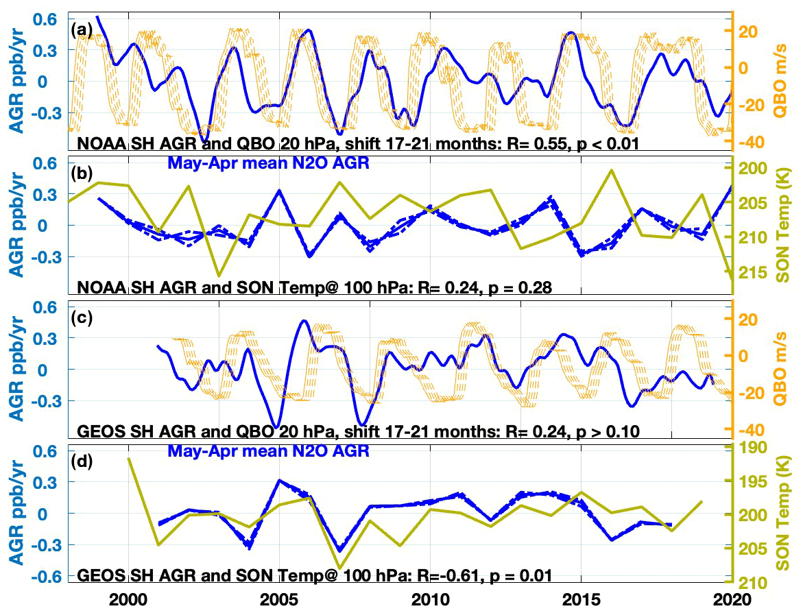
Figure 6 SH N₂O atmospheric growth rate (AGR in ppb yr⁻¹) for (a) NOAA and (c) GEOSCCM plotted with the QBO index at 20 hPa with a 17–21-month forward shift in the index. (b, d) SH N₂O AGR plotted with mean lower stratospheric temperature averaged over 60–90° S for September–November in the year prior to the annual label on the x axis. The AGR is averaged from monthly N₂O data over the ensuing 12-month period May–April (solid blue line), shifted plus or minus 1 month (dotted blue lines), for (b) NOAA and (d) GEOSCCM. Note that to convert to percentage per year (AGR units often used in the literature) parts per billion per year can be multiplied by 100/323, where 323 is the mean tropospheric mixing ratio of N₂O over 1998–2020.

In contrast to the SH, PLST in the NH from the previous winter is not correlated significantly to N₂O monthly anomalies at extratropical surface sites for either NOAA or GEOSCCM in any of the months surrounding the NH N₂O seasonal minimum, with the exception of Mace Head, Ireland, where a negative correlation is found in July in GEOSCCM (Fig. S3).

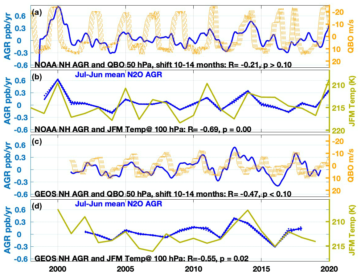
Figure 7 NH N₂O atmospheric growth rate (AGR in ppb yr⁻¹) for (a) NOAA and (c) GEOSCCM plotted with the QBO index at 50 hPa with a 10–14-month forward shift in the index. (b, d) NH N₂O AGR plotted with mean lower stratospheric temperature averaged over 60–90° N for January–March of the year labeled on the x axis. The AGR is averaged from monthly N₂O data over the encompassing 12-month period July–June (solid blue line), shifted plus or minus 1 month (dotted blue lines), for (b) NOAA and (d) GEOSCCM.

4 Discussion

The atmospheric N₂O observations and model results assembled here present several new lines of evidence that the stratosphere helps drive the seasonal minimum in tropospheric N₂O and also influences its atmospheric growth rate. First, the vertical cross sections of atmospheric N₂O from aircraft provide a broadscale perspective, in which N₂O-poor air enters the winter polar lower stratosphere, crosses the tropopause around the time of polar vortex breakup, and descends downward and equatorward, reaching Earth's surface by summer or early fall. These patterns are seen in both the NOAA empirical background and in global airborne survey data (Figs. 3, 4, 5). Second, GEOSCCM simulations show similar three-dimensional patterns to those in the NOAA empirical background (Fig. 3) and also yield correlations between the surface N₂O AGR with internally modeled QBO and PLST indices that are similar to those found in observations (Figs. 6, 7). In addition, GEOSCCM predicts correlations between February surface N₂O anomalies and PLST in the SH both for total N₂O similar to those observed and for the tagged stratospheric tracer N₂O_ST (Fig. 9).

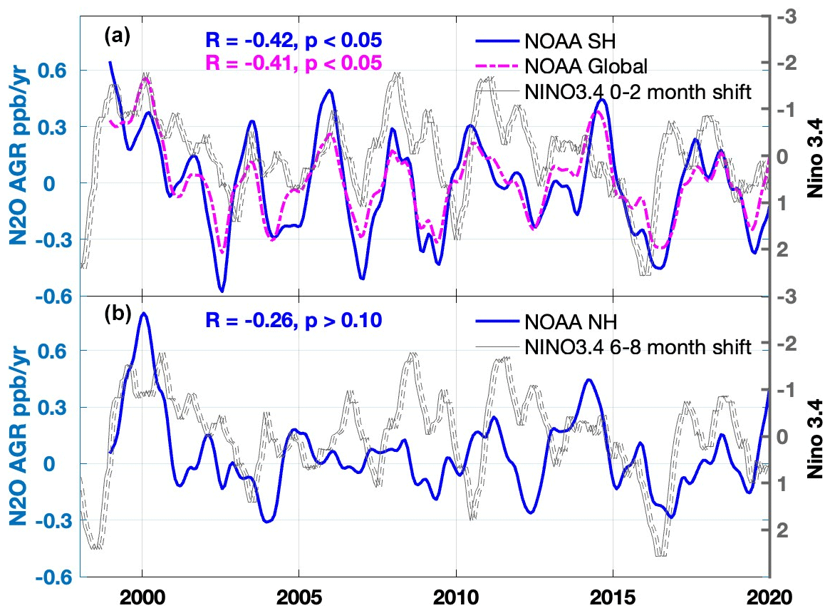
Figure 8 NOAA N₂O atmospheric growth rate (AGR in ppb yr⁻¹) plotted with the Niño 3.4 index for (a) SH and global mean AGR with a 0–2-month shift in the index and (b) NH AGR with a 6–8-month shift in the index.

The comparison of GEOSCCM output to NOAA observations, while qualitatively supporting a stratospheric influence on the troposphere, also raises questions. The phasing of the GEOSCCM N₂O seasonal cycle is delayed relative to observations, especially in the NH, and the model simulates a delay in propagating stratospheric signals down to the surface that is too long (Figs. 1, 3). Diabatic descent in the stratosphere has been shown to be underestimated in atmospheric models (e.g., Brühl et al., 2007; Khosrawi et al., 2009, 2018), and this may also be the case for air crossing into the troposphere. Another issue is that the seasonality of surface N₂O emissions may not be well represented in the GEOSCCM simulation. For example, summer soil emissions are from a soil biogeochemistry model and may be overestimated, leading to unrealistic surface maxima in July (Saikawa et al., 2013; Nevison et al., 2018; Liang et al., 2022).

With respect to the aircraft data, the NOAA empirical background and QCLS vertical cross sections, while showing similar features, are not matched exactly for comparison. QCLS data are measured across a narrow longitude band of the flight track for any given latitude on a limited number of days, while the NOAA empirical background is shown as a monthly mean, zonally averaged across most of the Western Hemisphere (170–50° W). Consequently, QCLS data are more likely to display synoptic-scale variability, such as the apparent surface source plume over the Southern Ocean seen in Fig. 10.

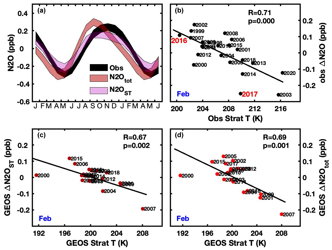
Figure 9 The top row shows (a) mean seasonal cycles in N₂O for NOAA surface station observations (Obs) and GEOSCCM surface total N₂O (N₂O_tot) and stratospheric N₂O (N₂O_ST), with uncertainty estimated using a bootstrap method, and (b) NOAA surface seasonal anomalies of N₂O mixing ratio (ppb) in February at the South Pole spanning 1998–2020, plotted vs. mean lower stratospheric MERRA-2 temperature at 100 hPa averaged over 60–90° S over the previous spring (September–November). The labeled anomalies in 2016 and 2017 correspond to the year of the ORCAS and ATom-2 aircraft surveys, respectively. The bottom row shows GEOSCCM surface seasonal anomalies of N₂O mixing ratio (ppb) for (c) N₂O_ST and (d) N₂O_tot in February at the South Pole spanning 2000–2019, plotted vs. mean GEOSCCM lower stratospheric temperature, which is sampled the same way as the MERRA-2 temperature.

4.1 Correlation to stratospheric indices: signs and magnitudes

The results of the correlation analysis based on NOAA surface N₂O data are similar to those found in previous studies based on Advanced Global Atmospheric Gases Experiment (AGAGE) surface N₂O data (Prinn et al., 2000; Nevison et al., 2007, 2011). In general, these correlations are weak, in part because the variability in surface N₂O is very small compared to its mean tropospheric mixing ratio. Nevertheless, PLST in the NH correlates significantly to NOAA surface N₂O AGR anomalies (Fig. 7b), and PLST in the SH correlates significantly to monthly N₂O anomalies in February near the time of the seasonal N₂O minimum (Fig. 9b). The negative sign of these correlations is easily understood and consistent with more downward transport of N₂O-poor air and warming of the polar lower stratosphere in years with stronger BDC, with subsequent cross-tropopause transport that deepens the descent of tropospheric N₂O into its seasonal minimum and slows the observed AGR of surface N₂O.

The reason for the positive correlation of the QBO index with the SH surface N₂O AGR (Fig. 6a, c) is less obvious. A similar correlation in the SH (but not the NH) has been observed in other studies but not fully explained (Ray et al., 2020). In our analysis, the positive correlation between the QBO and the SH N₂O AGR is strongest for the QBO at 20 hPa with 18 months lag and then weakens with decreasing QBO altitude down to 100 hPa, with a concurrent decrease in the optimal lag, likely due to the time needed for downward propagation of QBO winds (Fig. S4). At 50 hPa, we find an optimal lag time of 10–12 months (R=0.39), consistent with Ray et al. (2020) (who only presented results for QBO = 50 hPa).

Photochemical destruction of N₂O is highest when QBO winds above 30 hPa are in the westerly (positive) phase and lower-altitude QBO winds are in the easterly (negative) phase. This configuration is associated with increased vertical upwelling in the tropical lower stratosphere, which transports more N₂O to its peak loss region around 32 km (Strahan et al., 2021; Ruiz et al., 2021). Thus, the magnitude of QBO-associated photochemical destruction per se cannot be the main driver of the stratospheric influence on surface N₂O, since one would logically expect a negative correlation (i.e., slower growth in the troposphere due to more stratospheric N₂O loss during positive QBO). Ruiz et al. (2021) similarly concluded that surface variability in N₂O is not correlated directly to the QBO-driven variability in stratospheric loss but rather by dynamical variations in cross tropopause fluxes of air, which are governed at least in part by the BDC.

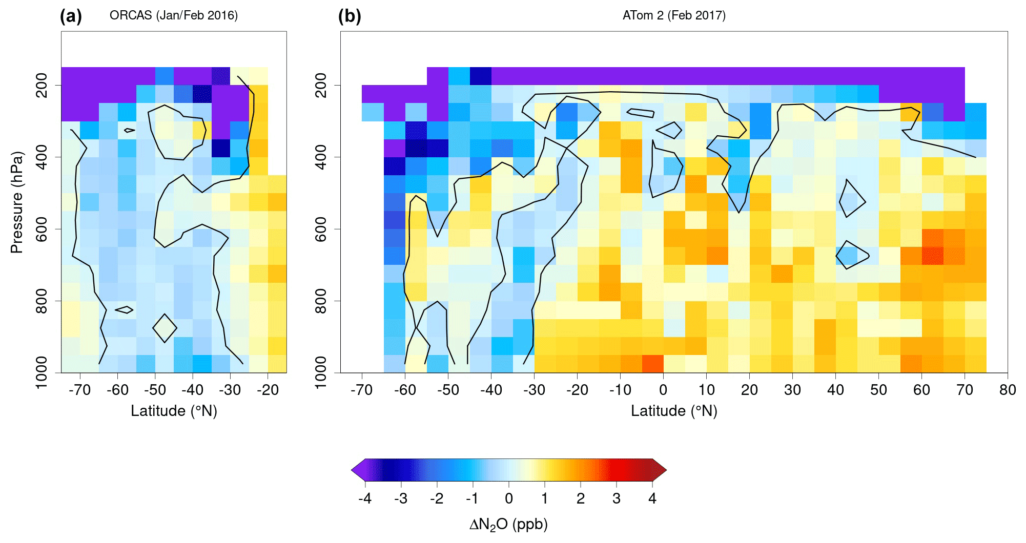
Figure 10 Anomalies of N₂O in parts per billion as a function of altitude and latitude from (a) ORCAS (Jan–Feb 2016) and (b) ATom-2 (Jan–Feb 2017).

The dynamics of the QBO, its interaction with the BDC and ultimate influence on surface N₂O are complex. However, the positive correlation of QBO, peaking at 20 hPa, with the SH N₂O AGR, could be explained in the context of Strahan et al. (2015), as described in detail in Sect. S2. Briefly, the QBO has an associated meridional circulation, which transports N₂O-poor air poleward from the region of peak photochemical destruction in the tropics between about 30 and 10 hPa in altitude. Paradoxically, this meridional circulation transports less N₂O-poor air toward the poles during the phase when the QBO is positive above 30 hPa (i.e., when photochemical destruction is highest). The N₂O-poor air subsequently is trapped in the Antarctic polar vortex and undergoes BDC-driven diabatic descent in isolation from mixing with lower latitudes, arriving largely intact in the lower stratosphere and eventually at Earth's surface, with a long lag time consistent with the 18-month lag found in Fig. 6a.

In the NH, the planetary wave activity that drives the BDC is stronger due to the more variable topography and stronger land-sea contrasts. Consequently, the BDC-driven descent into the winter pole is more strongly seasonal and the NH polar vortex is less isolated (Holton et al., 1995; Scaife and James, 2000; Butchart, 2014; Kidston et al., 2015), such that any signal associated with the QBO meridional circulation does not transport intact to lower altitudes (Strahan et al., 2015). This may explain why, for both NOAA surface stations and GEOSCCM, the NH N₂O AGR is more strongly correlated to PLST (a proxy for the BDC) than it is to the QBO, consistent with Ruiz et al. (2021).

In contrast to the NH, the NOAA SH surface N₂O AGR does not correlate to PLST. This result is somewhat puzzling given the significant correlation between PLST and NOAA N₂O February anomalies at SH high-latitude surface sites (Fig. 9). It appears that the impact of the stratosphere in austral summer as tropospheric N₂O descends into its seasonal minimum is not sufficient to influence the N₂O AGR across the whole SH over the entire year. The SH N₂O AGR results may reflect the strong preservation of the QBO signal that is ultimately transported into the troposphere, as discussed above, combined with the relatively weak BDC in the SH and/or the interference of ENSO-driven signals discussed below.

4.2 Correlations with ENSO

The NOAA surface station N₂O AGR correlation with the ENSO index is significant in the SH ($R=-\mathrm{0.42}$, p<0.05, 0–2-month phase shift) but weaker in the NH ($R=-\mathrm{0.26}$, p>0.10, 7-month optimal phase shift) (Fig. 10). The correlation in the SH could in part reflect meteorological shifts in the tropical low-level convergence pattern during positive (El Niño) conditions. For atmospheric gases with a positive north–south latitudinal gradient, these shifts result in a lessened influence of winds from the NH on the tropical SH and an increased influence of southeasterly winds. The NOAA Samoa site at 14° S, which strongly influences the cosine-latitude-weighted SH average, is known to be affected by these kinds of wind shifts (Prinn et al., 1992; Nevison et al., 2007). The fact that the N₂O AGR correlation with ENSO is considerably weaker in the NH than in the SH suggests a limited impact of ENSO on NH N₂O and supports the hypothesis that reduced north-to-south transport during positive ENSO contributes to the correlation observed in the SH.

The negative correlation between N₂O AGR and ENSO also may reflect a true reduction in the biogeochemical N₂O source during the positive ENSO phase, for example, due to drought over tropical land or due to reduced upwelling in the tropical ocean (Ishijima et al., 2009; Thompson et al., 2013). The most well-documented biogeochemical response of N₂O to ENSO events occurs in the eastern tropical South Pacific (ETSP), a well-known oxygen minimum zone (OMZ) and hot spot of oceanic N₂O emissions (Areivalo-Martinez, 2015; Ji et al., 2019). El Niño conditions decrease upwelling in the ETSP, thereby reducing the surface productivity, deepening the oxycline, contracting the OMZ, and decreasing the N₂O sea-to-air flux (Ji et al., 2019; Babbin et al., 2015).

However, less than a quarter of the total N₂O budget likely comes from oceanic emissions, of which the ETSP is only one component (Yang et al., 2020; Canadell et al., 2021). This raises questions about whether a reduced ETSP source (or a strengthened source during La Niña periods) has enough leverage to control the overall N₂O AGR. Ruiz et al. (2021) removed the stratospheric influence from surface N₂O data to infer a source of ∼ 1 Tg N (about 5 % of the total annual N₂O source) associated with the 2010 La Niña event, which could have come from tropical land or ocean, or some combination of both. Similarly, Kort et al. (2011) found evidence of strong episodic pulses of ∼ 1 Tg N from tropical regions, based on maxima in QCLS N₂O data measured in the middle and upper troposphere during aircraft campaigns in 2009. These pulses were not tied specifically to an ENSO event but rather more generally demonstrated the strength of the tropical N₂O source.

5 Summary and outlook

GEOSCCM simulations with a tagged stratospheric tracer show that N₂O-poor air descends throughout the winter into the polar lower stratosphere, crosses the tropopause in spring or early summer, and descends downward and equatorward, transmitting a diluted but still coherent signal to Earth's surface in late summer to early autumn (August–September in the NH, April–May in the SH). The GEOSCCM simulations are corroborated by N₂O observations from aircraft, which provide direct evidence for a stratospheric influence on tropospheric N₂O that previously was inferred primarily based on correlations of surface N₂O data to stratospheric indices. In support of the model and aircraft results and consistent with previous studies, significant correlations are found between the N₂O AGR observed at long-term NOAA surface monitoring sites and either the QBO index in the SH or PLST in the NH, where PLST is a proxy for the strength of the BDC. Correlations between the N₂O AGR and ENSO indices are also statistically significant in the SH, suggesting a joint influence of ENSO and the stratosphere on the AGR in that hemisphere. The QBO influences the rate at which N₂O is transported to and destroyed in the tropical stratosphere, but complex atmospheric dynamics buffer how variations in the N₂O photochemical loss rate are transmitted across the tropopause to modulate the surface N₂O AGR. Cross-tropopause transport at high latitudes is linked closely to the BDC and appears to be a more direct influence than the QBO on the N₂O AGR in the NH. In the SH in contrast, the combination of a better-preserved QBO signal and weaker BDC may lead to a direct (albeit with a ∼18-month lag) correlation between the QBO and the SH N₂O surface AGR, consistent with current knowledge of stratospheric dynamics.

The solar cycle is an additional influence on variability in N₂O that may be worth investigating in future work. While previous studies have estimated a relatively small effect over the 2000s and 2010s due to low solar activity (Ruiz et al., 2021; Prather et al., 2023), solar-cycle-driven changes in the UV flux affect N₂O photolysis both directly and indirectly through the impact stratospheric O₃. Another important issue is the impact on N₂O of climate-change-driven increases in the strength of the BDC (Garny et al., 2013; Butchart, 2014; Fu et al., 2019). Of particular relevance to the results presented here are studies based on ground- or satellite-based N₂O observations that find a decrease in the N₂O lifetime (Prather et al., 2023) and interhemispheric differences in stratospheric N₂O trends (Minganti et al., 2022). Finally, to help refine our understanding of variability in tropospheric N₂O, long-term monitoring at surface and aircraft-based sites is essential and would be complemented by more global airborne surveys extending into the lower stratosphere. The latter provide new insights into stratospheric influences on tropospheric N₂O and advance our ability to interpret and quantify surface N₂O sources.