Cloud water adjustments to aerosol perturbations are buffered by solar heating in non-precipitating marine stratocumuli

Marine low-level clouds are key to the Earth's energy budget due to their expansive coverage over global oceans and their high reflectance of incoming solar radiation. Their responses to anthropogenic aerosol perturbations remain the largest source of uncertainty in estimating the anthropogenic radiative forcing of climate. A major challenge is the quantification of the cloud water response to aerosol perturbations. In particular, the presence of feedbacks through microphysical, dynamical, and thermodynamical pathways at various spatial and temporal scales could augment or weaken the response. Central to this problem is the temporal evolution in cloud adjustment, governed by entangled feedback mechanisms. We apply an innovative conditional Monte Carlo subsampling approach to a large ensemble of diurnal large-eddy simulation of non-precipitating marine stratocumulus to study the role of solar heating in governing the evolution in the relationship between droplet number and cloud water. We find a persistent negative trend in this relationship at night, confirming that the role of microphysically enhanced cloud-top entrainment. After sunrise, the evolution in this relationship appears buffered and converges to $\sim -\mathrm{0.2}$ in the late afternoon. This buffering effect is attributed to a strong dependence of cloud-layer shortwave absorption on cloud liquid water path. These diurnal cycle characteristics further demonstrate a tight connection between cloud brightening potential and the relationship between cloud water and droplet number at sunrise, which has implications for the impact of the timing of advertent aerosol perturbations.

1 Introduction

Marine stratocumulus (Sc) clouds, found ubiquitously over subtropical oceans, are key to the Earth's radiation budget (Wood, 2012). They cool the Earth effectively through reflecting a considerable amount of incoming solar radiation (Bender et al., 2011; Stephens et al., 2012). The radiative effect of marine stratocumulus is governed by its macrophysical properties, such as areal coverage and liquid water path (LWP), and microphysical properties, such as cloud droplet number concentration (N_d) or drop size. Increases in atmospheric aerosol particles lead to an increase in smaller cloud droplets (Twomey, 1974, 1977); modulate the rate of warm cloud processes, e.g., collision–coalescence and entrainment mixing; and subsequently cause adjustments in cloud macrophysical properties (e.g., Albrecht, 1989; Bretherton et al., 2007; Wang et al., 2003; Xue and Feingold, 2006). The radiative forcing attributed to cloud adjustments in response to anthropogenic aerosol increases is currently poorly constrained, especially for marine boundary layer clouds, and remains the largest source of uncertainty in projections of the future climate (Boucher et al., 2013; Forster et al., 2021; Bellouin et al., 2020).

A key, yet uncertain, component of these cloud adjustments is the response of cloud water to aerosol perturbations. Constraining it is particularly challenging because the impact of aerosol on cloud LWP is bidirectional and regime-dependent (Chen et al., 2014; Gryspeerdt et al., 2019; Possner et al., 2020; Toll et al., 2019). For precipitating clouds, an increase in aerosol tends to increase LWP through precipitation suppression (Albrecht, 1989), whereas for non-precipitating clouds, LWP decreases through enhanced turbulent entrainment of dry, free-tropospheric (FT) air at cloud top, attributed to smaller droplets (Bretherton et al., 2007; Wang et al., 2003). Thus, the frequency of occurrence of different cloud states governs the overall response of cloud water to aerosol perturbations, which depends strongly on large-scale meteorological conditions (e.g., Zhang et al., 2022; Zhou et al., 2021; Zhang and Feingold, 2023).

Making the quantification of the LWP adjustment to aerosol perturbations even more challenging is the presence of feedbacks among system-wide microphysical, dynamical, and thermodynamical processes at different spatiotemporal scales, acting to buffer the system's response to perturbations (Stevens and Feingold, 2009). Quantifying aerosol effects on LWP in such a buffered system requires understanding not only of individual causal mechanisms but also of their timescales (Glassmeier et al., 2021; Fons et al., 2023; Gryspeerdt et al., 2022). Therefore, characterizing the temporal evolution of cloud adjustments is central to this problem, as it provides a way to assess the relative importance of individual mechanisms. Based on an ensemble of nocturnal large-eddy simulations (LESs) of marine stratocumulus, Glassmeier et al. (2021) suggested that the estimated cooling effect due to aerosol–cloud interactions derived from ship-track observations may be an overestimation if the temporal evolution in cloud water adjustment is not taken into account. Using satellite observations, Gryspeerdt et al. (2021) showed that the N_d–LWP relationship between ship tracks and their surroundings is indeed time-dependent and sensitive to the cloud and meteorological states under which the aerosol perturbation occurs. More generally, studies using geostationary satellites (e.g., Qiu et al., 2024; Christensen et al., 2023; Smalley et al., 2024) and polar-orbiting satellites (e.g., Diamond et al., 2020; Zhang and Feingold, 2023) have indicated diurnal variation in cloud adjustments to aerosol perturbations, such that LWP adjustments become more negative in the afternoon. Through extrapolating the Terra (late morning) and Aqua (early afternoon) difference, Gryspeerdt et al. (2022) demonstrated the importance of controlling initial cloud states to account for feedbacks in the system and found a negative, but weaker, N_d–LWP relationship when feedbacks are accounted for.

When it comes to the attribution of the diurnal variation in cloud adjustment to aerosol perturbations, an often overlooked, yet important, process is the shortwave (SW) absorption in the cloud layer. The balance between SW heating and longwave (LW) cooling plays a crucial role in governing the daytime evolution of cloud water in marine stratocumulus (e.g., Sandu et al., 2008; Chen et al., 2024). Since cloud SW absorption is a strong function of LWP and also dependent on N_d (Petters et al., 2012), it can potentially act as an important feedback (or “buffering”, in the case of a negative feedback) mechanism as cloud water changes throughout the sunlit hours.

In this study, we aim to characterize the diurnal evolution in cloud water adjustments to aerosol perturbations, with a particular focus on understanding the importance of SW absorption in affecting this evolution. We have performed a large ensemble of diurnal simulations of non-precipitating marine stratocumulus that represents conditions in the northeastern Pacific region, using an LES model that resolves aerosol–cloud interactions. By applying a novel subsampling approach (introduced in Sect. 2), we find that cloud SW absorption acts to flatten the N_d–LWP relationship (indicated by the regression slope) after sunrise, suggesting a buffered evolution in cloud water response to aerosol perturbations (Sect. 3.1). Enlightened by these results, we further use the subsampling approach to demonstrate a tight connection between the potential for cloud brightening and the cloud water–droplet number relationship at sunrise (Sect. 3.2). This has implications for the optimal timing of deliberate aerosol perturbations in the context of marine cloud brightening (MCB), one of the proposed climate intervention approaches (National Academies of Sciences, Engineering, and Medicine (NASEM) report, 2021; Latham and Smith, 1990; Latham et al., 2012), to the extent that they are constrained by the duration and the prescribed, time-invariant large-scale conditions of these simulations.

2 Methods and data

While process-model-based perturbation experiments help a great deal in understanding the causal mechanisms driving cloud adjustments to aerosol perturbations (e.g., Prabhakaran et al., 2023, 2024; Chun et al., 2023), these studies are typically limited in their ability to represent the range of boundary layer conditions observed in nature. A new approach in the most recent decade suggests that one can infer process-level understanding from the systematic behavior of simulation ensemble(s) that depict the evolution of cloud systems from a wide range of initial boundary layer conditions (e.g., Glassmeier et al., 2019, 2021; Hoffmann et al., 2020, 2023), as a way to bridge “Newtonian” (bottom-up) and “Darwinian” (top-down) approaches (Feingold et al., 2016; Mülmenstädt and Feingold, 2018). Following this methodology, we analyze a large ensemble of diurnal simulations of marine stratocumulus with an innovative subsampling approach, in which the large ensemble is sub-grouped into smaller ensembles as a means to investigate the impact of N_d on cloud water evolution and how it is mediated by SW heating.

2.1 Large-eddy simulation ensemble of marine stratocumulus

All simulations used in this study are carried out with the System for Atmospheric Modeling (SAM; Khairoutdinov and Randal, 2003). The model domain size is set to $\mathrm{48}\times \mathrm{48}\times \mathrm{2.5}$ km³ with a horizontal and vertical grid spacing of 200 and 10 m, respectively. This setup allows for development of mesoscale organizations (Kazil et al., 2017) while keeping computational cost affordable for a large ensemble of simulations. All simulations are run for 24 h from 18:40 local time right after sunset at a time step of 1 s. Cloud microphysical processes are simulated with a two-moment, bin-emulating bulk microphysical scheme (Feingold et al., 1998) with prognostic total number concentration and total water content (Yamaguchi et al., 2019). Aerosol number concentration (N_a) is prescribed to be initially uniform throughout the domain, and we assume a lognormal aerosol size distribution (ammonium sulfate) with a geometric-mean diameter of 0.2 µm and geometric standard deviation of 1.5 µm, following Feingold et al. (2016). Aerosol particles are lost to cloud and precipitation processing, such as collision–coalescence, scavenging, and wet deposition, and we apply a constant surface flux of aerosol of 70 cm⁻² s⁻¹ (Yamaguchi et al., 2017; Kazil et al., 2011) to mitigate depletion of aerosol. Radiative heating rates are calculated interactively every 10 s using the Rapid Radiative Transfer Model (RRTMG; Clough et al., 2005) with extended thermodynamic profiles above the domain top (2.5 km), following Yamaguchi et al. (2017). Surface sensible and latent heat fluxes are calculated interactively based on Monin–Obukhov similarity and initialized with climatological mean surface winds. We prescribe a constant sea surface temperature (SST) of 292.4 K, based on the ERA5-derived climatology of large-scale meteorological conditions associated with the stratocumulus deck off the coast of California (Hersbach et al., 2020) and a fixed large-scale divergence of $\mathrm{3.75}\times {\mathrm{10}}^{-\mathrm{6}}$ s⁻¹ (Ackerman et al., 2009) for all simulations. The reader is referred to Chen et al. (2024) for more technical details on the setup of the simulations.

Keeping the above model setup and large-scale forcings the same for all simulations, we vary the initial conditions for boundary layer (BL) thermodynamics in a six-parameter variable space to create ensemble members, using a maximin Latin hypercube sampling approach (Morris and Mitchell, 1995) to minimize correlations between parameters, as described in Feingold et al. (2016) and Glassmeier et al. (2019). The six parameters include BL liquid water potential temperature ($\mathrm{284}\le {\mathit{\theta }}_{\text{l}}\le \mathrm{294}$ K), the BL total water mixing ratio ($\mathrm{6.5}\le q_{\text{t}}\le \mathrm{10.5}$ g kg⁻¹), the jumps of temperature and humidity between BL and FT ($\mathrm{6}\le \mathrm{\Delta }{\mathit{\theta }}_{\text{l}}\le \mathrm{10}$ K and $-\mathrm{10}\le \mathrm{\Delta }{q}_{\text{t}}\le \mathrm{0}$ g kg⁻¹), the initial mixed-layer depth ($\mathrm{500}\le h_{\text{mix}}\le \mathrm{1300}$ m), and the aerosol number concentration ($\mathrm{30}\le N_{\text{a}}\le \mathrm{500}$ mg⁻¹). Using the Latin hypercube sampling approach, we generate hundreds of initial thermodynamic profiles, from which we carry out simulations whenever a cloud layer is produced and when the lifting condensation level is between 225 and 1075 m and the FT θ_l and q_t profiles are within the ERA5 climatology of the northeastern Pacific. This yields a total of 316 diurnal simulations. Since we focus on the non-precipitating marine stratocumulus system, we impose a threshold of 0.5 mm d⁻¹ on the cloud base rain rate to screen for non-precipitating simulations (Wood, 2012). We further exclude simulations that generate a surface fog, cloud tops higher than 2 km, and a domain cloud fraction (f_c) of less than 0.01 (full cloud dissipation) to ensure the robustness of our analysis when the subsampling is applied. Domain-mean 2-dimensional and 3-dimensional outputs are saved every 2 min and every hour, respectively. A total of 204 non-precipitating simulations are selected for analysis. We discard the first 4 h of all simulations as model spin-up and use a cloud optical depth (τ) threshold of 1 to identify clouds. A higher threshold of τ=5 was tested but did not change the conclusions qualitatively.

2.2 A conditional Monte Carlo sampling approach

Many recent studies (e.g., Gryspeerdt et al., 2016, 2019; Glassmeier et al., 2021; Zhang et al., 2022; Zhou et al., 2021; Smalley et al., 2024) have chosen to infer the impact of aerosol on cloud properties by examining the spatiotemporal correlation between cloud macrophysical properties and N_d, with N_d serving as an intermediate variable, in order to mitigate the influence of confounding factors on the causal relationship between aerosol and clouds and to avoid uncertainties in relating aerosol information, such as aerosol optical depth and aerosol index, to cloud condensation nuclei (CCN; Stier, 2016). Here, we adopt the same methodology and focus on the relationship between N_d and LWP, quantified as the slope of linear regressions (e.g., McComiskey and Feingold, 2012). Least-squares log regressions are used to alleviate the dependence of the regression slope on the absolute value of N_d (e.g., Feingold et al., 2003; Zhang et al., 2022).

Nevertheless, covarying meteorological and aerosol conditions can still confound the N_d–LWP relationship in observations (e.g., Gryspeerdt et al., 2019) and in model simulations (e.g., Mülmenstädt et al., 2024). Therefore, we introduce a subsampling approach that can be conditioned on prescribed relationships among N_d, LWP, and initial boundary layer conditions, following the Monte Carlo methodology (Hammersley and Handscomb, 1964), with modifications to enable selection of specified conditions. We term this subsampling approach “conditional Monte Carlo (cMC).” The fundamental idea of employing the Monte Carlo concept is to use repetitive, semi-random (i.e., conditional) samplings to capture systematic behaviors (deterministic in principle) of stochastically initialized realizations of marine Sc evolution. The purpose of the cMC approach in this work is threefold. First, it serves to help constrain the covariation between N_d and meteorological conditions under which the simulations are initialized, which could confound the effect of N_d on LWP. Second, it serves as a means to free ourselves from dealing with an initially positive (after spin-up) N_d–LWP relationship imposed purely by the Latin hypercube sampling used to construct the initial boundary layer conditions. Third, we use it to select N_d–LWP relationships and observe their temporal evolution. In this work, we use statistical regression slopes to indicate the relationship (not necessarily causal) between two variables (e.g., N_d and LWP). The application of the cMC method alleviates the concern of whether statistical slopes can indicate causal relationships, as we focus on the evolution rather than the absolute value of these slopes by selecting a range of slopes at sunrise.

The cMC approach is applied as follows. We first randomly draw 25 simulations from the 204 LES ensemble members (non-precipitating), using a random seed generator assuming a normal distribution. The “conditional” part of cMC is implemented such that a drawing is saved only when the following conditions are met: first, the covariation between N_d and three boundary layer conditions (abbreviated as MET hereafter) at the beginning of the simulation (4 h) is smaller than user-imposed thresholds (i.e., minimizing the correlation between N_d and MET after spin-up). These three variables are cloud-top height (z_ct; a measure of boundary layer depth), surface sensible heat flux (SHF), and 800 hPa relative humidity (RH₈₀₀), and the thresholds are $-\mathrm{0.05}\le \mathrm{d}\ln \left(z_{\text{ct}}\right)/\mathrm{d}\ln \left(N_{\text{d}}\right)\le \mathrm{0.05}$, $-\mathrm{0.5}\le \mathrm{d}\text{SHF}/\mathrm{d}\ln \left(N_{\text{d}}\right)\le \mathrm{0.5}$, and $-\mathrm{0.05}\le \mathrm{d}\ln \left({\text{RH}}_{\mathrm{800}}\right)/\mathrm{d}\ln \left(N_{\text{d}}\right)\le \mathrm{0.05}$. Second, the N_d–LWP regression slope is close enough, within uncertainty ranges, to a user-prescribed value – essentially prescribing a cloud water–droplet number relationship for the randomly drawn 25 simulations. In our first investigation (Sect. 3.1), we prescribe five values for the N_d–LWP slope ($\mathrm{d}\ln \left(\text{LWP}\right)/\mathrm{d}\ln \left(N_{\text{d}}\right)$) at sunrise, ±0.4 (±0.02), ±0.2 (±0.01), and 0 (±0.005), to examine the role of SW heating. In our second investigation (Sect. 3.2), we prescribe flat slopes for N_d–LWP and N_d–f_c, i.e., $-\mathrm{0.005}\le \mathrm{d}\ln \left(\text{LWP}\right)/\mathrm{d}\ln \left(N_{\text{d}}\right)\le \mathrm{0.005}$ and $-\mathrm{0.05}\le \mathrm{d}{f}_{\text{c}}/\mathrm{d}\ln \left(N_{\text{d}}\right)\le \mathrm{0.05}$, to mimic the relationship between cloud micro- and macrophysical properties at the time of aerosol perturbation, representing a difference in the timescale between the “instantaneous” (order of minutes) microphysical response and the slower (order of hours) macrophysical adjustments. In order to maintain practical sampling efficiency of the cMC approach while approximating desired regression slopes, we impose arbitrary bounding values (or thresholds) around the desired slopes without any threshold on the correlation coefficient between N_d and LWP. We note that our approach is not designed to select a narrow, linear band of points in ln (LWP)–ln (N_d) space but rather relies on the correlation between N_d–LWP to infer the relationship between them, given the relatively large number of samples in each sub-ensemble.

Within each 25-member subgroup of simulations, we calculate the slope between N_d and LWP as $\mathrm{d}\ln \left(\text{LWP}\right)/\mathrm{d}\ln \left(N_{\text{d}}\right)$ at each time step. We focus on the temporal evolution in $\mathrm{d}\ln \left(\text{LWP}\right)/\mathrm{d}\ln \left(N_{\text{d}}\right)$, in particular on the difference between nighttime and sunlit hours (Sect. 3.1) and the impact of N_d–LWP relationship at sunrise on time-integrated cloud radiative effect (Sect. 3.2), rather than the absolute value of $\mathrm{d}\ln \left(\text{LWP}\right)/\mathrm{d}\ln \left(N_{\text{d}}\right)$, which we prescribe when subsampling. The drawing is repeated with the same pre-conditions but different random number seeds to produce 50 25-member subgroups, and the mean evolution (averaged over 50 repetitions) is shown in the results. We also tested other configurations of the cMC setup, varying the number of members within each draw, number of draws, and the user-imposed thresholds. Different configurations yield the same conclusions, qualitatively, and the choice of the current configuration is based on sampling efficiency.

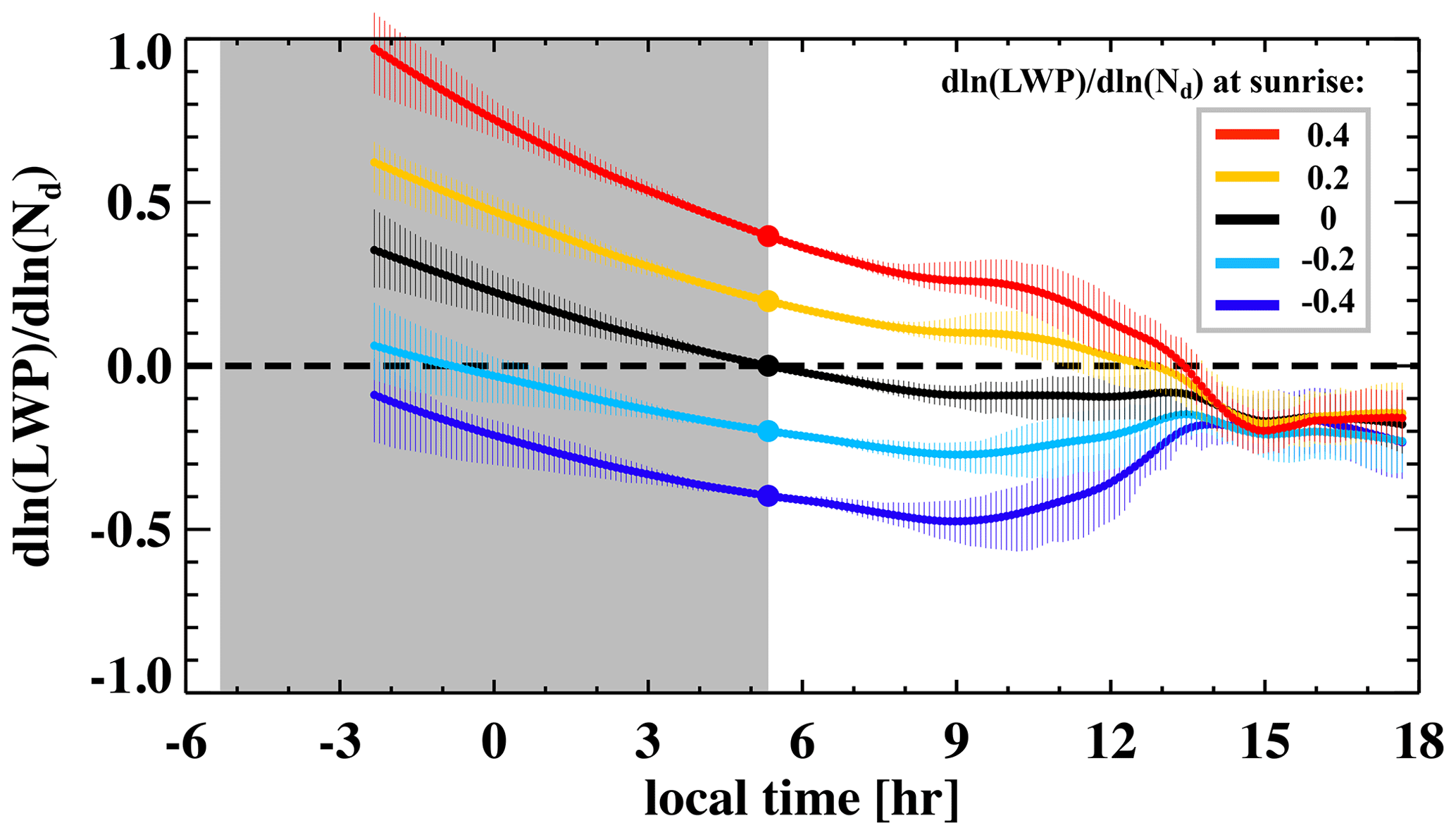
Figure 1 Diurnal cycle of the N_d–LWP regression slope ($\mathrm{d}\ln \left(\text{LWP}\right)/\mathrm{d}\ln \left(N_{\text{d}}\right)$). Solid lines indicate mean values of the 50 25-member cMC subsampling for individual groups, which are separated by colors representing different $\mathrm{d}\ln \left(\text{LWP}\right)/\mathrm{d}\ln \left(N_{\text{d}}\right)$ values at sunrise (large dots). Vertical bars indicate interquartile ranges for each group. A 1 h running mean is applied. Gray shading indicates nighttime hours.

3 Results

3.1 The role of SW absorption in affecting diurnal evolution in the N_d–LWP relationship

3.1.1 A buffered evolution during the daytime

Besides the variations in N_d being a fundamental perturbation to the Sc system, the impact of solar heating on cloud water evolution starting from sunrise is another important perturbation to the system. During daytime, the sensitivity of radiation to cloud macro- and microphysical properties is critical to the evolution in the N_d–LWP slope. In particular, the dependence of cloud-layer LW cooling on LWP and N_d is only apparent in thin clouds and saturates at around 20 to 30 g m⁻², whereas SW heating increases continuously as LWP and N_d increase, more pronouncedly with LWP (Petters et al., 2012). The different sensitivities of solar heating to LWP and N_d, which vary among LES ensemble members, are hypothesized to affect the daytime evolution in the N_d–LWP slope. In order to examine the effects of solar heating on the cloud water–droplet number relationship, using the cMC approach, we subsample five conditions where subsampled simulations possess prescribed N_d–LWP slopes at sunrise, ranging from −0.4 to 0.4 with an increment of 0.2 (Sect. 2.2). The diurnal evolution in the N_d–LWP slope (and correlation coefficient) of the five subgroups is shown in Fig. 1 (and Fig. S1 in the Supplement), with the red curve indicating the most positive (0.4) N_d–LWP slope at sunrise and the blue curve representing the most negative (−0.4) one. A persistent feature of the N_d–LWP slopes becoming more negative with time is observed at night, consistent with the findings in Glassmeier et al. (2021), regardless of the prescribed slopes at sunrise. This is attributed to the sensitivity of turbulent entrainment at cloud top to drop size, such that smaller drops (higher N_d) promote stronger entrainment. A sensitivity of the entrainment mechanism to LWP is also evident in the nighttime evolution where the decrease in the N_d–LWP slope for the group that starts with an initially positive N_d–LWP slope (higher N_d associated with higher LWP) is faster (from 1 to 0.4, red), compared to that in the group starting with a negative slope (from −0.1 to −0.4, blue; Fig. 1).

Interesting evolution in the N_d–LWP slope appears a couple of hours after sunrise where groups starting from very different N_d–LWP slopes at sunrise begin to converge (Fig. 1). The group convergence shares features typical to buffered evolution, such that the groups starting with a negative slope become less negative, whereas the groups starting with a positive slope become less positive over time. We will show that the cause of such a buffered evolution during the day is the primary dependence of SW heating on cloud LWP, such that thicker clouds (higher LWP) experience stronger cloud thinning with stronger SW absorption, whereas thinner clouds thin more slowly with weaker SW absorption, leading to flattening of all N_d–LWP slopes, regardless of their values at sunrise. For this task, we will need to quantify the rate of change in LWP attributed to radiative processes. Hence, we performed a budget analysis of the LWP tendency, following Chen et al. (2024), to further illustrate this attribution in the following.

3.1.2 The sensitivity of LWP tendency to N_d

The impact of N_d perturbations on cloud LWP is through affecting the rates of processes that govern the budget of cloud water. Here, we focus on two terms in this budget that are known to be sensitive to cloud water and droplet number, namely entrainment and radiation processes, derived as below, following Chen et al. (2024). First, the total rate of change of cloud LWP is written as

$$\begin{array}{}\text{(1)}& {\mathcal{L}}^{\prime }={\mathrm{\Gamma }}_{\text{l}}\langle {\mathit{\rho }}_{\mathrm{0}}\rangle (z_{\text{inv}}-z_{\text{cb}})\left[z_{\text{inv}}^{\prime }-\left({\displaystyle \frac{\mathrm{d}{z}_{\text{cb}}}{\mathrm{d}\langle q_{\text{t}}\rangle }}\langle q_{\text{t}}{\rangle }^{\prime }+{\displaystyle \frac{\mathrm{d}{z}_{\text{cb}}}{\mathrm{d}\langle {\mathit{\theta }}_{\text{l}}\rangle }}\langle {\mathit{\theta }}_{\text{l}}{\rangle }^{\prime }\right)\right],\end{array}$$

where ℒ denotes LWP, ^′ denotes time derivatives, z_cb is the mean cloud base height, z_inv is the mean inversion base height, and Γ_l is the liquid water adiabatic lapse rate. We then decompose 〈q_t〉^′ and 〈θ_l〉^′ into individual budget terms grouped by processes ($\langle \mathit{\varphi }{\rangle }_{\text{process}}^{\prime }$), e.g., radiation (RAD) and entrainment (ENT). 〈ϕ〉 is the volume mean of a scalar quantity that represents either q_t or θ_l in our case. In particular, $\langle \mathit{\varphi }{\rangle }_{\text{RAD}}^{\prime }$ is straightforwardly calculated from the 3-dimensional, modeled radiative heating rates, and $\langle \mathit{\varphi }{\rangle }_{\text{ENT}}^{\prime }$ is approximated by the difference between the total tendency of 〈ϕ〉 in the boundary layer (BL) and the sum of contributions from all processes other than ENT, which can be directly estimated from the modeled fields. The reader is referred to Chen et al. (2024) for more details on the derivation and justification of assumptions for the LWP tendency budget analysis.

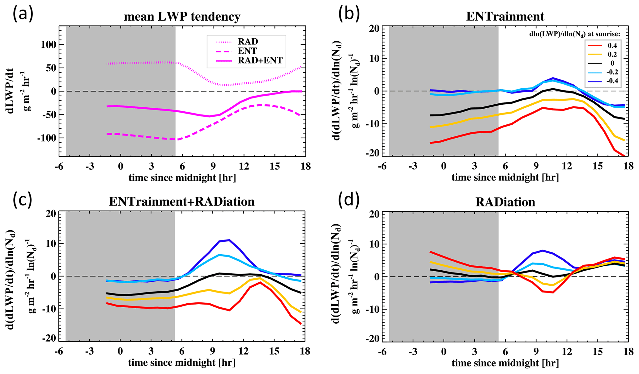
Figure 2 Diurnal cycle of (a) mean LWP tendencies attributed to radiation (RAD), entrainment (ENT), and the sum of RAD and ENT (RAD + ENT) and (b–d) their sensitivity to N_d. Mean sensitivity evolution is shown for the five groups with different prescribed N_d–LWP relationships ($\mathrm{d}\ln \left(\text{LWP}\right)/\mathrm{d}\ln \left(N_{\text{d}}\right)$) at sunrise, whose evolution in $\mathrm{d}\ln \left(\text{LWP}\right)/\mathrm{d}\ln \left(N_{\text{d}}\right)$ is shown in Fig. 1. A 1 h running mean is applied. Gray shading indicates nighttime hours.

First, we show the mean evolution in LWP tendencies attributed to entrainment, radiation, and their net effect (Fig. 2a). ${\mathcal{L}}_{\text{RAD}}^{\prime }$ remains constant throughout the night, consistent with the saturation of the dependence of LW cooling on LWP when clouds are still relatively thin. ${\mathcal{L}}_{\text{ENT}}^{\prime }$ strengthens weakly as cloud thickens during the night. After sunrise, SW heating offsets LW cooling and weakens the entrainment mixing at cloud tops. During cloud recovery in the late afternoon, the impacts of radiation and entrainment on LWP tendency balance each other. We caution that during the late afternoon the difference between the ℒ^′ from the budget analysis (i.e., Eq. 1) and the ℒ^′ diagnosed directly from the simulations increases, and for this reason, we limit our interpretation of the LWP budget evolution to the hours before 15:00 local time.

Next, we investigate the sensitivity of LWP tendency to N_d (i.e., ${\mathcal{L}}_{\text{ENT}}^{\prime \prime }$, ${\mathcal{L}}_{\text{RAD}}^{\prime \prime }$, and ${\mathcal{L}}_{\text{ENT+RAD}}^{\prime \prime }$, where the second ^′ indicates derivatives with respect to ln (N_d); Fig. 2b–d), focusing on their role in governing the evolution in $\mathrm{d}\ln \left(\text{LWP}\right)/\mathrm{d}\ln \left(N_{\text{d}}\right)$, as seen in Fig. 1. Different colors in Fig. 2b–d represent exactly the same subgroups conditioned on prescribed values of $\mathrm{d}\ln \left(\text{LWP}\right)/\mathrm{d}\ln \left(N_{\text{d}}\right)$ at sunrise, i.e., from −0.4 to 0.4. An important note to keep in mind is that these sensitivities to N_d inherently include sensitivities to LWP because we prescribed the N_d–LWP slope in these subgroups, such that high N_d is associated with high LWP when $\mathrm{d}\ln \left(\text{LWP}\right)/\mathrm{d}\ln \left(N_{\text{d}}\right)$ is positive (e.g., the red line), and high N_d is associated with low LWP for a negative $\mathrm{d}\ln \left(\text{LWP}\right)/\mathrm{d}\ln \left(N_{\text{d}}\right)$ (e.g., the blue line).

During the night, the net effect of entrainment and radiation on the LWP tendency (Fig. 2c) nicely explains the persistent decreasing trend in $\mathrm{d}\ln \left(\text{LWP}\right)/\mathrm{d}\ln \left(N_{\text{d}}\right)$ (Fig. 1). The negative values in ${\mathcal{L}}_{\text{ENT+RAD}}^{\prime \prime }$ (regardless of the prescribed $\mathrm{d}\ln \left(\text{LWP}\right)/\mathrm{d}\ln \left(N_{\text{d}}\right)$ values) suggest that clouds with higher N_d experience stronger LWP loss, resulting in the N_d–LWP slope becoming more negative with time. This effect is primarily driven by the ${\mathcal{L}}_{\text{ENT}}^{\prime \prime }$ term (Fig. 2b), consistent with the entrainment-enhancement mechanism due to more smaller droplets (Wang et al., 2003). When cloud water and droplet number are positively correlated (the red line), the sensitivity of the LWP tendency to N_d (${\mathcal{L}}_{\text{ENT+RAD}}^{\prime \prime }$) is found to be the strongest (Fig. 2c), confirming the fastest decrease in $\mathrm{d}\ln \left(\text{LWP}\right)/\mathrm{d}\ln \left(N_{\text{d}}\right)$ in that subgroup (Fig. 1), as both higher N_d and higher LWP induce stronger entrainment.

After sunrise, a feature essential to explaining the buffered evolution in $\mathrm{d}\ln \left(\text{LWP}\right)/\mathrm{d}\ln \left(N_{\text{d}}\right)$ emerges, that is ${\mathcal{L}}_{\text{ENT+RAD}}^{\prime }$ in subgroups with a negative $\mathrm{d}\ln \left(\text{LWP}\right)/\mathrm{d}\ln \left(N_{\text{d}}\right)$ at sunrise (i.e., blue and cyan) become positively correlated with N_d (Fig. 2c), indicating a reverse of the persistent nighttime negative trend in $\mathrm{d}\ln \left(\text{LWP}\right)/\mathrm{d}\ln \left(N_{\text{d}}\right)$, which leads to the flattening of the negative N_d–LWP slopes (Fig. 1). Radiation, especially SW heating, plays a critical role here by dominating the contribution to the stratification feature observed in ${\mathcal{L}}_{\text{ENT+RAD}}^{\prime \prime }$ between 10:00 and 11:00 local time (Fig. 2d). This would not be the case if ${\mathcal{L}}_{\text{RAD}}^{\prime \prime }$ were to follow its trend during the nighttime as if there were no solar radiation. The dependence of solar heating on N_d and especially cloud water is key. Unlike LW cooling, whose dependence on LWP saturates when clouds are still relatively thin, the dependence of SW heating on LWP persists in thicker clouds (Petters et al., 2012), such that thick clouds absorb more SW than thin clouds – a positive slope between SW heating and LWP. This leads to a negative slope between ${\mathcal{L}}_{\text{RAD}}^{\prime }$ and LWP, given that LW cooling still dominates the contribution of radiative processes to the LWP tendency in the daytime; i.e., ${\mathcal{L}}_{\text{RAD}}^{\prime }$ is positive in the mean (Fig. 2a, red line). In other words, higher LWP induces more SW heating or stronger offsetting of the LW cooling, leading to a weaker LWP tendency due to radiation. Effectively, the inclusion of SW radiation reverses the slope between ${\mathcal{L}}_{\text{RAD}}^{\prime }$ and N_d, regardless of the prescribed N_d–LWP slope (Fig. 2d). When a positive N_d–LWP slope is imposed at sunrise, this translates into a negative slope between ${\mathcal{L}}_{\text{RAD}}^{\prime }$ and N_d (red line in Fig. 2d), whereas when N_d and LWP are negatively correlated, ${\mathcal{L}}_{\text{RAD}}^{\prime \prime }$ is positive (Fig. 2d, blue line). The fact that the dependence of ${\mathcal{L}}_{\text{RAD}}^{\prime }$ on LWP is able to explain the observed evolution in ${\mathcal{L}}_{\text{RAD}}^{\prime \prime }$ suggests that the effect of N_d on the LWP tendency driven by radiative processes is secondary to the impact of LWP. In other words, if the counterhypothesis is true, that is the N_d impact is not secondary to the LWP impact (or comparable to the LWP impact), then ${\mathcal{L}}_{\text{RAD}}^{\prime \prime }$ should be skewed towards negative values after sunrise, as the LWP impact and the N_d impact offset (complement) each other in the case of a negative (positive) N_d–LWP slope. Therefore, we conclude that the buffered evolution observed in $\mathrm{d}\ln \left(\text{LWP}\right)/\mathrm{d}\ln \left(N_{\text{d}}\right)$ after sunrise (Fig. 1) can be attributed to the primary dependence of SW heating on cloud water.

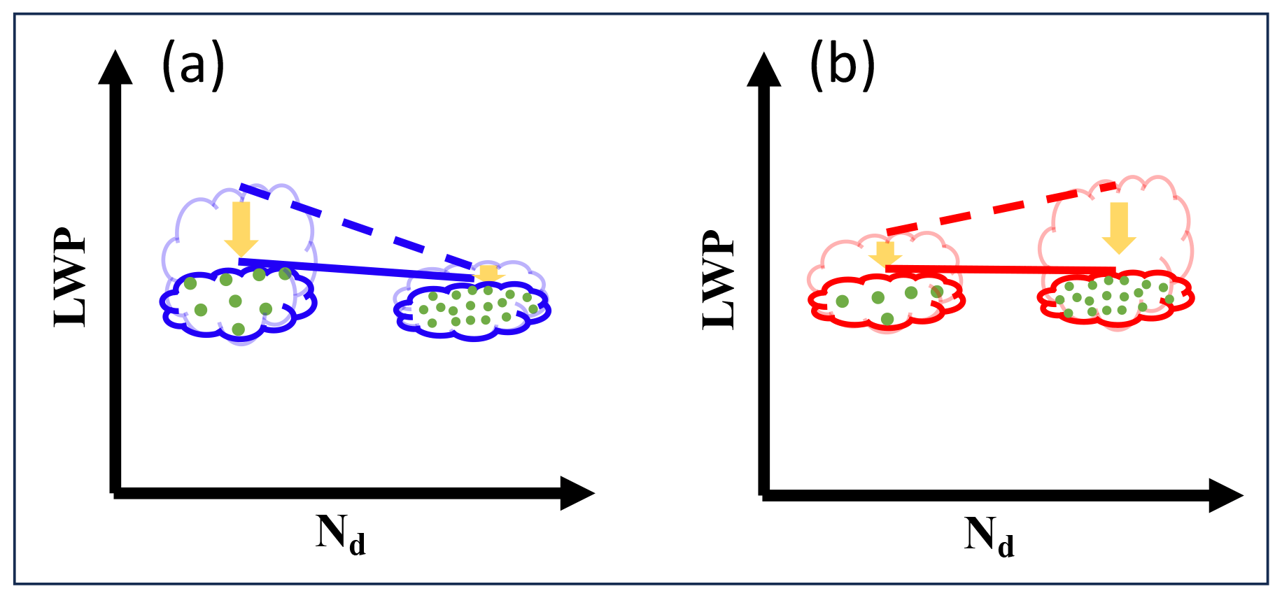
Figure 3 A schematic illustrating the hypothesis for the cause of the buffered daytime evolution in N_d–LWP relationship – that is thicker clouds thin faster, whereas thinner clouds thin slower, resulting in flattened slopes (solid lines) regardless of the initial slope at sunrise (dashed lines). Blue (red) “clouds” represent the blue (red) group in Fig. 1.

To summarize, we have identified two features associated with the diurnal evolution of the cloud water–droplet number relationship for non-precipitating Sc: (1) the N_d–LWP slope becomes more negative with time at night, and (2) the N_d–LWP slope flattens (is buffered) after sunrise due to the strong dependence of SW heating on cloud LWP than on N_d. A schematic summarizing the latter point is shown in Fig. 3, where thicker clouds (higher LWP) experience stronger cloud thinning, resulting in flattening of the N_d–LWP slope. Keeping these two features in mind, we next explore the dependence of the cloud radiative effect, in the form of daytime-integrated SW reflection, on the relationship between cloud water and droplet number at sunrise.

3.2 The role of the N_d–LWP relationship at sunrise in governing the daytime cloud radiative effect

When we assess the radiative effect at the top of the atmosphere (TOA) due to aerosol–cloud interactions (ACIs), the reflectance from the entire Sc scene matters. In other words, the all-sky SW albedo of the cloud field is governed by its areal coverage (f_c) and the optical thickness of the cloud, which is a function of its LWP and N_d (i.e., $\mathit{\tau }\propto {\text{LWP}}^{\frac{\mathrm{5}}{\mathrm{6}}}{N}_{\text{d}}^{\frac{\mathrm{1}}{\mathrm{3}}}$, based on the adiabatic assumption; Boers and Mitchell, 1994). Using a two-stream approximation to relate changes in cloud albedo (A_c) to changes in τ (Platnick and Twomey, 1994), one can show that the sensitivity of A_c to N_d perturbations (S) follows the form of

$$\begin{array}{}\text{(2)}& S={\displaystyle \frac{\mathrm{d}{A}_{\text{c}}}{\mathrm{d}\ln \left(N_{\text{d}}\right)}}={\displaystyle \frac{A_{\text{c}}(\mathrm{1}-A_{\text{c}})}{\mathrm{3}}}(\mathrm{1}+{\displaystyle \frac{\mathrm{5}}{\mathrm{2}}}{\displaystyle \frac{\mathrm{d}\ln \left(\text{LWP}\right)}{\mathrm{d}\ln \left(N_{\text{d}}\right)}}).\end{array}$$

Clearly, one sees that the subject of this study – the cloud water–droplet number relationship ($\mathrm{d}\ln \left(\text{LWP}\right)/\mathrm{d}\ln \left(N_{\text{d}}\right)$) – is central to this equation, in the sense that close to −0.4 it could determine the sign of S, i.e., cloud brightening or darkening. As demonstrated in the previous section, diurnal evolution in $\mathrm{d}\ln \left(\text{LWP}\right)/\mathrm{d}\ln \left(N_{\text{d}}\right)$ is sensitive to its value at sunrise. This motivates us to further investigate the effect of the N_d–LWP slope at sunrise on the daytime cloud radiative effect due to N_d perturbations. Given the persistent decreasing trend in $\mathrm{d}\ln \left(\text{LWP}\right)/\mathrm{d}\ln \left(N_{\text{d}}\right)$ during the night (Fig. 1), assuming unchanged large-scale meteorological conditions throughout the day, one can relate the sunrise value of $\mathrm{d}\ln \left(\text{LWP}\right)/\mathrm{d}\ln \left(N_{\text{d}}\right)$ to the elapsed time since the perturbation in N_d was introduced. This is because at the time when an aerosol perturbation is applied to a Sc system, we know that N_d responds to the addition of aerosol much more quickly than the amount of cloud water and its horizontal extent (i.e., cloud fraction) adjust to the new microphysical state of the cloud, resulting in a flat slope between cloud micro- and macrophysical properties. As a result, the earlier the N_d perturbation is applied, the more negative $\mathrm{d}\ln \left(\text{LWP}\right)/\mathrm{d}\ln \left(N_{\text{d}}\right)$ will be at sunrise, as $\mathrm{d}\ln \left(\text{LWP}\right)/\mathrm{d}\ln \left(N_{\text{d}}\right)$ persistently decreases during the night.

We use the cMC method to subsample conditions where a 25-member subset of the LES ensemble has near-zero N_d–LWP and N_d–f_c slopes, to mimic flat slopes between cloud micro- and macrophysical properties, in addition to the constraint on N_d–MET covariations. (See Sect. 2.2 for the threshold values used to impose these constraints.) We vary the time at which we impose these near-zero slopes, ranging from 22:40 to 05:40 (∼ sunrise) local time with an increment of 1 h, yielding eight subsampled groups whose diurnal evolution in the slope between cloud properties (LWP, f_c, A_c, and SW reflection) and N_d is further examined. Although our opportunistic sampling strategy based on background aerosol conditions does not fully represent deliberate aerosol seeding, such as MCB, which will likely inject larger and more hygroscopic particles than we assumed in these simulations, it does provide insights into the qualitative relationship between MCB efficacy and seeding time.

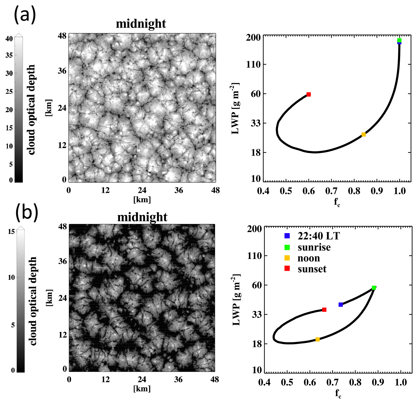
Figure 4 Left column: example 2D snapshots of cloud optical depth at local midnight (hour 6 of the simulation time) and right column: mean diurnal cycle of LWP and cloud fraction (f_c) of the simulated closed-cell and (non-precipitating) open–cell Sc. Sunrise, sunset, noon, and 22:40 LT (end of spin-up) are indicated on the diurnal cycle.

A subtlety here is the interpretation of N_d–f_c relationships (quantified as $\mathrm{d}{f}_{\text{c}}/\mathrm{d}\ln \left(N_{\text{d}}\right)$), as the diurnal evolution in f_c between open-cell (non-precipitating) Sc and closed-cell Sc is distinct from each other (e.g., Fig. 4). Besides, open-cell Sc clouds can have quite different cloud-top entrainment characteristics, compared to closed-cell clouds (e.g., Abel et al., 2020). For these reasons, we further classify the 204 non-precipitating cases into (1) overcast closed-cell Sc and (2) non-precipitating open-cell Sc, based on f_c values at night. A total of 114 simulations where f_c remains 1 from ∼ 22:40 (local time; after spin-up) to sunrise are classified into (1), and the rest (90 runs) are classified into (2). Figure 4 shows example snapshots of the cloud field at midnight and the mean cloud behaviors of these two classes. For overcast closed-cell Sc, clouds thin first while maintaining the overcast state before they start to break up at ∼100 g m⁻² (Fig. 4a). For non-precipitating open-cell Sc, clouds thicken and widen at the same time before sunrise, and, in a similar manner, they thin and shrink after sunrise, creating a loop-like diurnal cycle in the LWP–f_c variable space (Fig. 4b). Both classes of clouds begin to recover LWP and f_c after noon, except that the non-precipitating open-cell class recovers f_c faster.

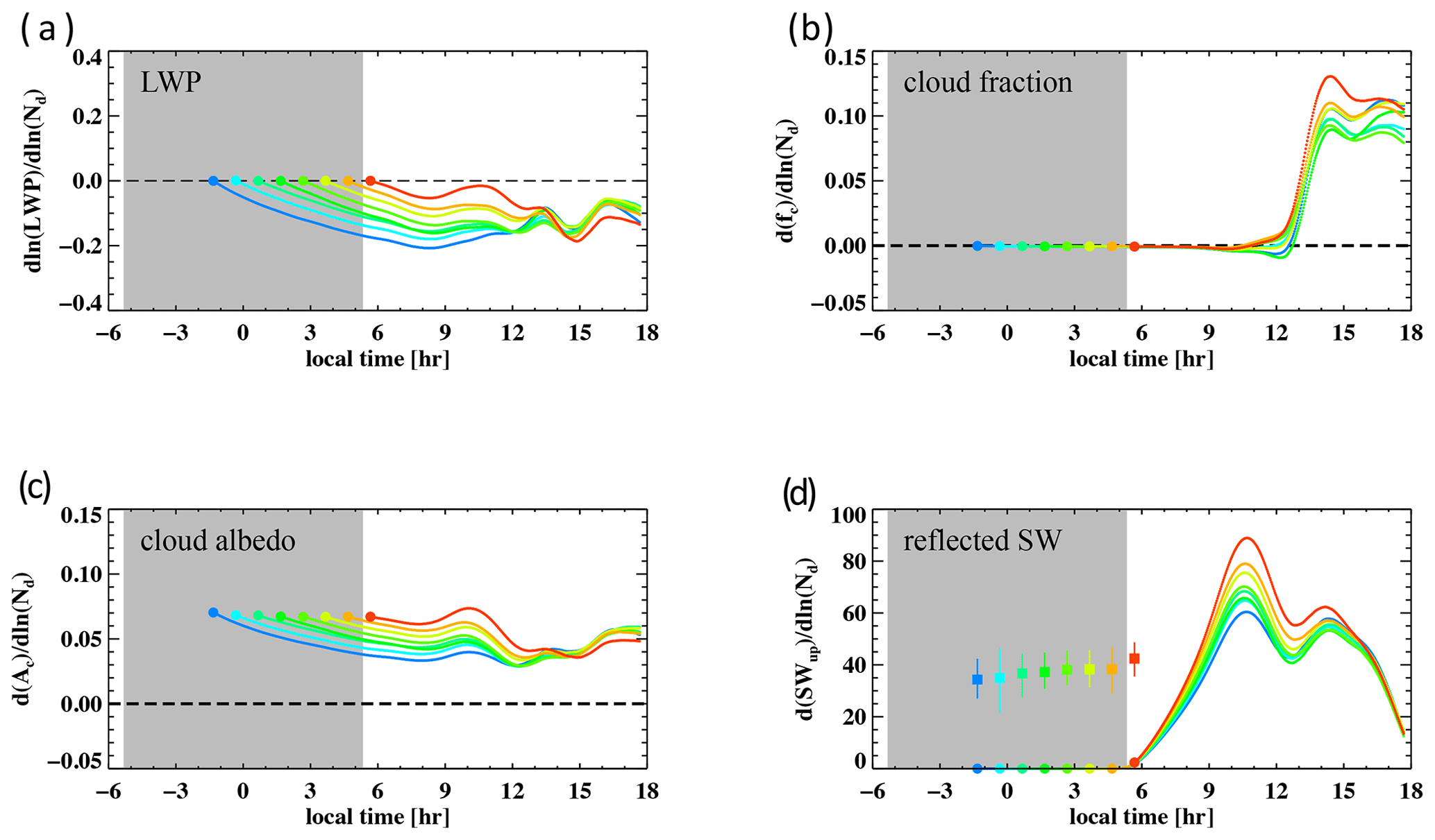
Figure 5 Diurnal cycle of (a) $\frac{\mathrm{d}\ln \left(\text{LWP}\right)}{\mathrm{d}\ln \left(N_{\text{d}}\right)}$, (b) $\frac{\mathrm{d}{f}_{\text{c}}}{\mathrm{d}\ln \left(N_{\text{d}}\right)}$, (c) $\frac{\mathrm{d}{A}_{\text{c}}}{\mathrm{d}\ln \left(N_{\text{d}}\right)}$, and (d) $\frac{\mathrm{d}{\text{SW}}_{\text{up}}}{\mathrm{d}\ln \left(N_{\text{d}}\right)}$. Colors separate groups mimicking “aerosol perturbation” at different times when $\frac{\mathrm{d}\ln \left(\text{LWP}\right)}{\mathrm{d}\ln \left(N_{\text{d}}\right)}$ and $\frac{\mathrm{d}{f}_{\text{c}}}{\mathrm{d}\ln \left(N_{\text{d}}\right)}$ are set to ∼0. Mean values averaged over 50 repeated cMC samplings of each group are shown. Relationships between N_d and diurnally integrated reflected SW (i.e., $\mathrm{d}(\int {\text{SW}}_{\text{up}}\mathrm{d}t)/\mathrm{d}\ln \left(N_{\text{d}}\right)$) for different perturbation times are shown as filled squares with interquartile ranges using the same color scheme. A 1 h running mean is applied. Gray shading indicates nighttime hours.

3.2.1 Overcast closed-cell Sc

Figure 5a–d show the evolution of slopes between N_d and cloud properties, including LWP, f_c, cloud albedo (A_c), and upwelling SW radiation at TOA (SW_up; a measure of reflected SW radiation by the entire cloud scene) for the eight cMC-subsampled groups (separated by colors). The N_d–LWP slope in all subgroups trends negatively with time during the night, and its evolution appears buffered after sunrise (Fig. 5a), consistent with the results shown in Sect. 3.1 (Fig. 1). The N_d–A_c slope is positive despite the negative N_d–LWP slope (Fig. 5c), in agreement with the critical N_d–LWP slope of −0.4 for the LWP adjustment to overcome the Twomey effect (Eq. 2). The evolution in the N_d–A_c slope closely tracks that in the N_d–LWP slope, suggesting a strong control of $\mathrm{d}\ln \left(\text{LWP}\right)/\mathrm{d}\ln \left(N_{\text{d}}\right)$ over S. The clouds remain overcast throughout the night until late morning, when the thinnest clouds break up earliest, resulting in a slight negative N_d–f_c slope, owing to the negative slope between N_d and LWP at sunrise, but only when $\mathrm{d}\ln \left(\text{LWP}\right)/\mathrm{d}\ln \left(N_{\text{d}}\right)$ is strongly negative (e.g., blue line in Fig. 5). This is also evident in the relationships between N_d and the cloud breakup time ($\mathrm{d}\left({\text{time}}_{f_{\text{c}}<\mathrm{0.95}}\right)/\mathrm{d}\ln \left(N_{\text{d}}\right)$), where only the two groups with the earliest perturbation time (thereby more negative $\mathrm{d}\ln \left(\text{LWP}\right)/\mathrm{d}\ln \left(N_{\text{d}}\right)$ at sunrise) do not show a delayed breakup (Fig. 6, black) under high-N_d conditions. After noon, the N_d–f_c slope becomes positive for all groups (Fig. 5b), attributed to a generally delayed diurnal cycle in both LWP and f_c (Fig. 6), meaning cloud thinning and breakup occur later in high-N_d clouds due to weaker LWP and f_c tendencies when N_d and LWP are negatively correlated at sunrise (Figs. 5a and S2).

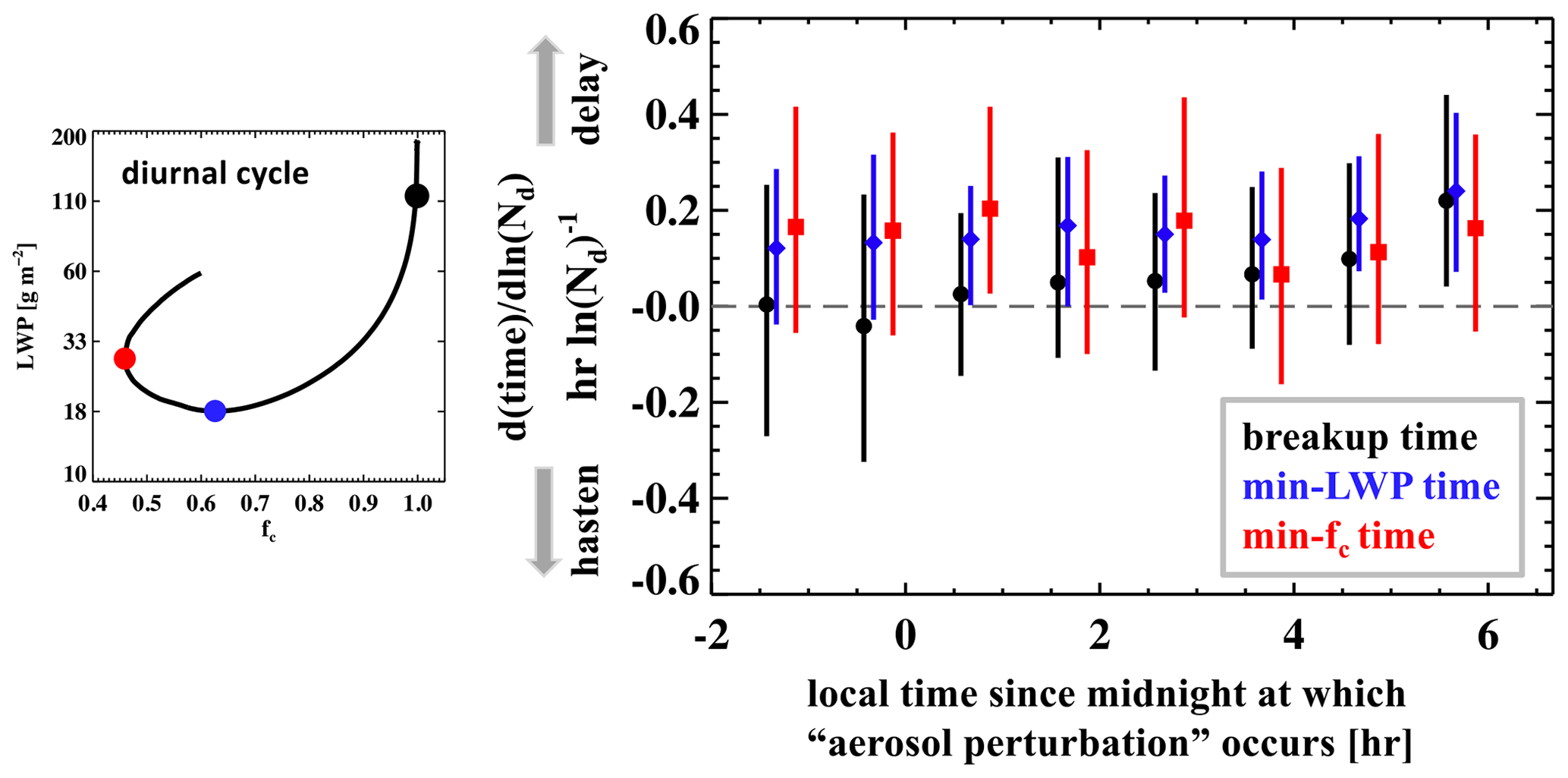
Figure 6 Relationships between N_d and overcast closed-cell Sc diurnal cycle critical times, i.e., $\mathrm{d}\left({\text{time}}_{\text{critical}}\right)/\mathrm{d}\ln \left(N_{\text{d}}\right)$, which include the time when cloud breaks up (f_c<0.95; black), reaches minimum LWP (blue), and reaches minimum f_c (red), for different “aerosol perturbation” times. Mean values and interquartile ranges are shown. The left-hand-side diagram is the same as that in Fig. 5a, for the illustration of critical times in the diurnal cycle.

When we combine the effects of Twomey, LWP, and f_c adjustments, it comes as no surprise that higher N_d leads to more reflected SW at TOA throughout the day (Fig. 5d), given that the negative $\mathrm{d}\ln \left(\text{LWP}\right)/\mathrm{d}\ln \left(N_{\text{d}}\right)$ is not strong enough to overcome the Twomey effect (Fig. 5c) and that $\mathrm{d}{f}_{\text{c}}/\mathrm{d}\ln \left(N_{\text{d}}\right)$ is mostly positive. Clearly, SW_up has the strongest sensitivity to N_d perturbations in the group with the latest “aerosol perturbation” (at sunrise; red line in Fig. 5d), which produces the greatest increase in the temporally integrated SW_up per unit increase in ln (N_d) (Fig. 5, filled squares). A critical difference between these groups is the N_d–LWP relationship at sunrise, which is important for daytime cloud tendencies and strongly tied to the time of “aerosol perturbation” in this setup.

Figure 7 As in Fig. 5 but for the non-precipitating open-cell Sc class.

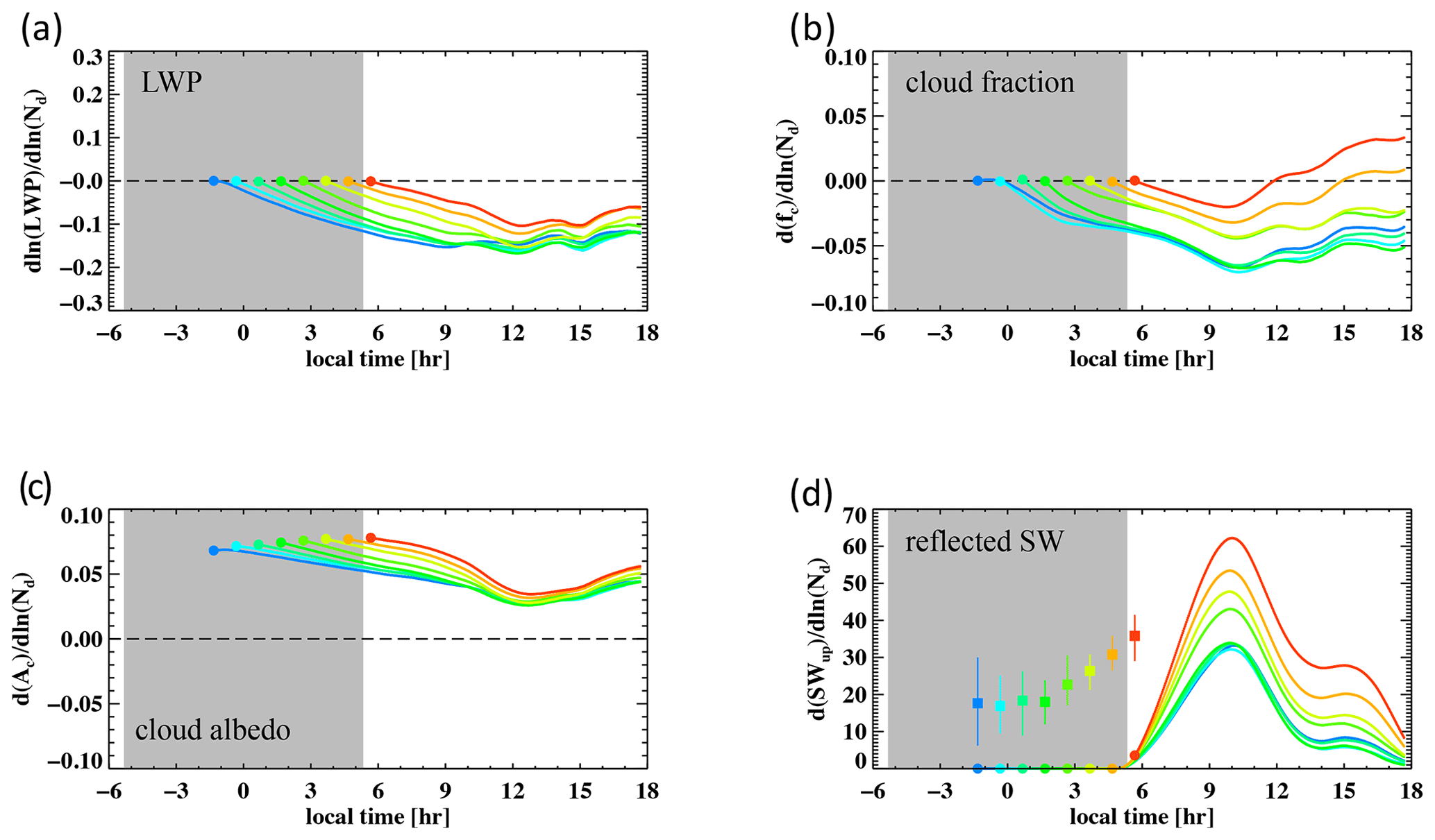
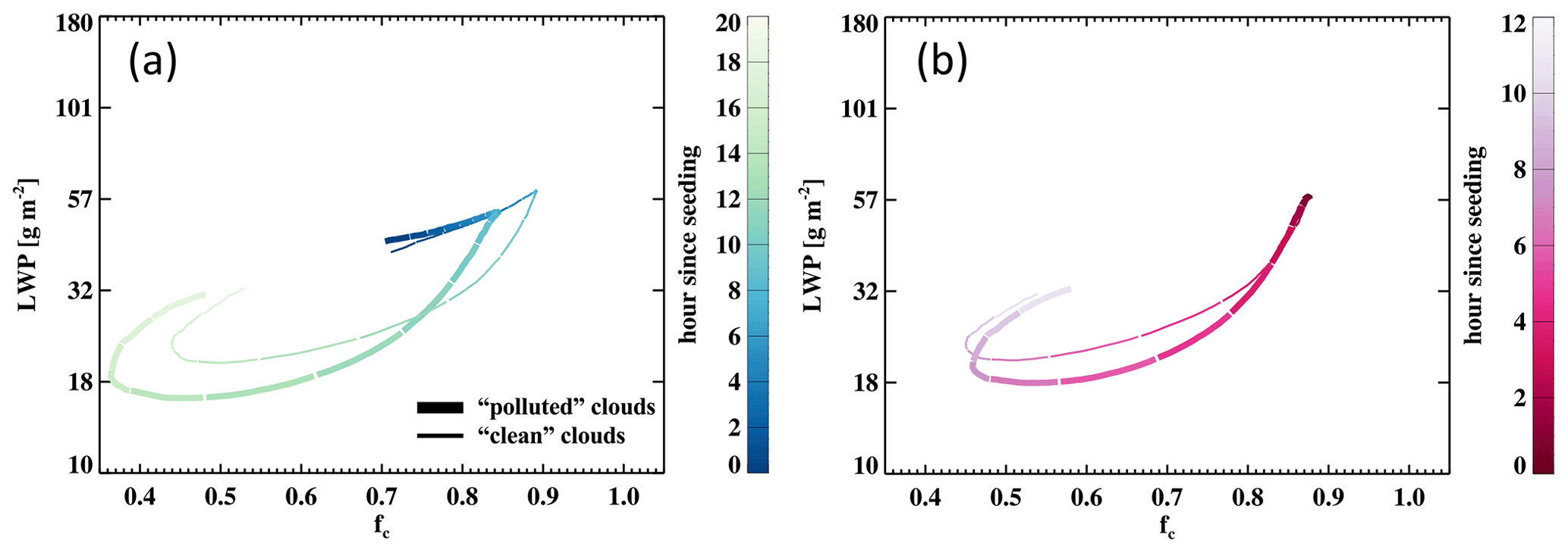
Figure 8 Diurnal cycle of cloud evolution in LWP–f_c space, for (a) the earliest and (b) the latest (at sunrise) “aerosol perturbation” groups. Thick lines represent the mean evolution of the highest 20 % of the members in N_d (“polluted” clouds, high-N_d), whereas the thinner lines indicate the lowest 20 % in N_d (“clean” clouds, low-N_d). Lines are colored and separated at every hour since the “aerosol perturbation”.

3.2.2 Non-precipitating open-cell Sc

Similar evolution in N_d–LWP and N_d–A_c slopes is found in non-precipitating open-cell Sc (Fig. 7a and c). In contrast to the evolution in N_d–f_c slope for the overcast closed-cell Sc, where different groups track each other quite closely throughout the day, the N_d–f_c slope after sunrise stratifies by both the N_d–LWP and the N_d–f_c slopes at sunrise in the non-precipitating open-cell Sc (Fig. 7b). This is consistent with the characteristic diurnal cycle of LWP and f_c (Fig. 4b) such that they increase (or decrease) coherently with time, leading to a similarly buffered evolution in $\mathrm{d}{f}_{\text{c}}/\mathrm{d}\ln \left(N_{\text{d}}\right)$ (Fig. 7b). Worth noting is that the buffering effect drives a sign change in $\mathrm{d}{f}_{\text{c}}/\mathrm{d}\ln \left(N_{\text{d}}\right)$ after noon for the groups with the latest “aerosol perturbation” (orange and red lines). A comparison between the earliest and the latest (at sunrise) “aerosol perturbation” groups (Fig. 8) reveals that for groups starting with already pronounced negative N_d–LWP and N_d–f_c slopes at sunrise (Fig. 8a), the effect of increasing N_d is to shift the diurnal cycle towards lower LWP and lower f_c in general. However, for groups where LWP and f_c remain similar between high- and low-N_d clouds at sunrise (Fig. 8b), the addition of smaller cloud droplets reduces LWP gradually, a process that can be attributed to the enhanced cloud-top entrainment, while similar f_c is maintained. For both cases, cloud recovery is noted to be slighted hastened under high-N_d conditions (Fig. S3), which is likely facilitated by weaker SW heating due to reduced LWP. In the case of sunrise “perturbation” where f_c is only subtly adjusted, hastened f_c recovery leads to a positive $\mathrm{d}{f}_{\text{c}}/\mathrm{d}\ln \left(N_{\text{d}}\right)$ in the afternoon (Figs. 7b and 8).

This stratification in N_d–f_c slopes complements the radiative impact due to N_d–LWP stratification alone (Fig. 7a), leading to an even more pronounced stratification in $\mathrm{d}{\text{SW}}_{\text{up}}/\mathrm{d}\ln \left(N_{\text{d}}\right)$ evolution. As a result, the dependence of $\mathrm{d}(\int {\text{SW}}_{\text{up}}\mathrm{d}t)/\mathrm{d}\ln \left(N_{\text{d}}\right)$ on “aerosol perturbation” time is more pronounced than that in the overcast closed-cell Sc (Fig. 7d, filled squares).

4 Discussion

Despite the wide usage of the statistical regression method to derive aerosol–cloud relationships from which process understanding is inferred, the extent to which these statistical relationships equate to a causal response, thereby representing cloud adjustments, has been a nagging concern of studies of this kind. More recently, there is evidence showing that the negative branch of the observed inverted-V shape in the N_d–LWP relationship (e.g., Gryspeerdt et al., 2019) overestimates the true causal effect of N_d on LWP (e.g., Arola et al., 2022; Fons et al., 2023). Using general circulation models (GCMs), Mülmenstädt et al. (2024) demonstrate the possibility that the sign of the cloud adjustment inferred from the N_d–LWP relationship derived from internal variabilities can even be misleading, which they attribute to the confounding effect of the covariation between N_d and meteorological conditions.

We wish to note that the way we investigate the relationship between cloud water and droplet number, i.e., by subsampling conditions where a subsample of the large simulation ensemble has a predetermined N_d–LWP relationship and by focusing on its evolution rather than its absolute value, alleviates reliance on the interpretation of the N_d–LWP relationships as causal relationships. In other words, the SW-heating-driven feedback (or buffering) mechanism we have uncovered in this work is a robust feature of the Sc system and does not depend on the actual (prescribed) value of $\mathrm{d}\ln \left(\text{LWP}\right)/\mathrm{d}\ln \left(N_{\text{d}}\right)$ in the cMC experiments or in the real world. From this perspective, we discuss the role that these results, in particular this feedback mechanism, play in the aerosol–cloud interactions that we observe in nature, where the N_d–LWP relationship is not predetermined and often confounded by other cloud controlling factors. In fact, a number of satellite-based studies have suggested that this relationship in nature is strongly dependent on cloud regime, boundary layer characteristics, and the spatial scale of one's investigation (e.g., Gryspeerdt et al., 2019; Possner et al., 2020; Toll et al., 2019; Zhou and Feingold, 2023). The essence of this radiation buffering is the dependence of LWP tendency attributed to radiation processes (SW absorption in particular) on cloud LWP, meaning thicker clouds thin faster and thinner clouds thin more slowly (Fig. 3), flattening whatever slope N_d and LWP may have had before sunrise, depending on the large-scale meteorological conditions the clouds have experienced, no matter whether the N_d–LWP relationship is causal or not.

Although many aspects of the boundary layer thermodynamic structure are varied to construct the large ensemble, two large-scale conditions, namely SST and free-troposphere subsidence, are fixed among ensemble members. The cMC approach is designed to effectively limit the role that the variability in these large-scale conditions can play in driving the evolution in the N_d–LWP relationship, by subsampling simulations with flat slopes between N_d and other cloud controlling factors at the beginning of the simulations. Although such a variability in the prescribed large-scale conditions can cause subtle differences in the exact timing and strength of the “buffered” feature, the finding of the feature itself remains robust based on a sensitivity test with variable SST simulations (not shown). Once again, the concept of using a large ensemble with cMC sampling is not to provide a reference value for the N_d–LWP relationship, which may still be weakly dependent on the prescribed SST and subsidence even after applying cMC, but to explore features of the Sc system that are robust even in the context of (co-)varying large-scale conditions, e.g., in the real world.

Moreover, one of the strengths of this novel subsampling approach is by design to minimize the confounding effects from the initial boundary layer conditions in this large ensemble of simulations and to address some of the aforementioned concerns. Therefore, although our emphasis is not on quantifying actual cloud adjustments, we aim to advance our understanding of the temporal evolution in adjustments. Consider the marine cloud brightening (MCB) idea, one of the proposed climate intervention approaches, as an example. When we think about how we might maximize the total amount of sunlight reflected over a day if we were to seed non-precipitating Sc clouds to increase their reflectivity of solar radiation, we want neither a negative LWP adjustment to start with nor seeding after the sun is up. Given the persistent negative trend in the nighttime evolution of $\mathrm{d}\ln \left(\text{LWP}\right)/\mathrm{d}\ln \left(N_{\text{d}}\right)$ (Fig. 1 and Sect. 3.1), it is logical to propose that seeding at sunrise would be the most effective brightening strategy, which our results in Sect. 3.2 have validated. This is attributed to the critical role of sunrise values of cloud water, N_d, and their correlation in governing the daytime evolution of cloud fraction and LWP.

There are, of course, caveats to this implication. For one, we focus only on non-precipitating Sc systems, whereas studies have shown that precipitation can modulate the impact of cloud-top entrainment on the LWP adjustment (Smalley et al., 2024; Stevens et al., 1998). Furthermore, suppressing or even preventing precipitation in Sc systems can potentially generate larger radiative impacts, compared to brightening the non-precipitating systems (e.g., Wang and Feingold, 2009; Prabhakaran et al., 2023, 2024; Chun et al., 2023). Moreover, given the typical lifetime of aerosol in the marine boundary layer (a few days; Wood, 2012, 2021), our integration over one diurnal cycle may seem short in terms of representing the full extent of the radiative impact due to seeding. Extending the analysis to three diurnal cycles by re-using the 24 h simulations for cMC subsampling results in similar conclusions with respect to the persistent nighttime negative trend in the N_d–LWP slope and the daytime buffering due to SW absorption, which essentially makes the N_d–LWP slope oscillate between −0.1 and −0.4 after convergence during the first afternoon (Fig. S4). That said, these non-precipitating Sc clouds tend to be advected by the prevailing winds in the region and experience pronounced large-scale forcing changes, e.g., warming SST and deepening marine boundary layer, which lead to transition into a more cumulus regime, during the course of 3 to 5 d over subtropical ocean basins (Bretherton and Wyant, 1997; Yamaguchi et al., 2017). Studies deploying large ensemble of multi-day Lagrangian simulations are warranted to further address this issue. While the implications of this particular exemplary application (i.e., MCB) are limited, the great potential of applying this cMC approach to simulation ensembles is demonstrated.

5 Conclusions

A novel conditional Monte Carlo (cMC) subsampling approach is applied to a large ensemble of diurnal LESs, in order to explore the role of solar heating in affecting the temporal evolution and timescale of cloud water adjustment to aerosol perturbations in non-precipitating marine stratocumulus. We find evidence supporting an important negative feedback (or buffering) mechanism in the daytime evolution of the N_d–LWP relationship such that a persistent decreasing trend at night is buffered (N_d–LWP slope becomes flattened) after sunrise, regardless of the actual value of $\mathrm{d}\ln \left(\text{LWP}\right)/\mathrm{d}\ln \left(N_{\text{d}}\right)$. Using a budget analysis of the LWP tendency, we separate and quantify the contributions from individual processes to this tendency, including entrainment and radiation. This enables us to attribute this buffering effect to the primary dependence of SW heating on LWP. This result emphasizes the dominant role of cloud LWP in governing daytime cloud tendencies, especially those related to SW absorption. The impacts of N_d perturbations appear to be only secondary.

This SW-LWP buffering has important implications for the temporal evolution in cloud adjustments to aerosol perturbations and the timescale of adjustments. Among various feedback mechanisms through microphysical processes, such as evaporation and sedimentation, surface fluxes, and/or large-scale circulation adjustments (e.g., Wang et al., 2003; Bretherton et al., 2007; Chun et al., 2023; Dagan et al., 2023), the role of SW heating has received the least attention. The implications for aerosol–cloud radiative forcing of climate are yet to be fully evaluated.

The methodology applied to the large simulation ensemble (i.e., subsampling) differs from previous studies in which the whole ensemble is used at once to map emergent properties, such as the cloud radiative effect (Glassmeier et al., 2019) and their flow field, from a wide range of initial conditions (e.g., Glassmeier et al., 2021; Hoffmann et al., 2020). This work demonstrates the substantial potential in the application of this cMC approach. It can enhance the usefulness of any large ensemble of simulations by generating numerous sub-ensembles, whose potential in scientific applications is well beyond that of the original ensemble, without the need to increase the size of the original ensemble.

The cMC subsampling approach presents a new pathway to explore systematic behaviors in cloud evolution from a large number of simulated realizations or observations while avoiding spurious covariations among cloud controlling factors that are related to either the seemingly random initializations or meteorological confounding factors. This alleviates the need to assume that spatiotemporal correlations can be used to infer causal relationships. Moreover, it enables one to select conditions where hypothesis-driven constraints can be prescribed and tested.

The SW-LWP buffering mechanism and its important role in governing the diurnal evolution in cloud water response to droplet number perturbations also have implications for the assessment of the viability of MCB. The robust decreasing trend in the N_d–LWP relationship at night motivates an MCB-oriented thinking on how one might maximize the sunlight reflected by a cloud scene. Using the cMC subsampling approach as a way to mimic the timing of the aerosol perturbation, we make the case that seeding at sunrise presents the highest potential for brightening. This statement is by no means an endorsement of MCB as a viable climate intervention method. Much more solid research is needed at this stage to determine the viability of MCB and to quantify the potential risks associated with it (Feingold et al., 2024).