the Creative Commons Attribution 4.0 License.
the Creative Commons Attribution 4.0 License.
 | 13 Sep 2024
Ozone anomalies over the polar regions during stratospheric warming events
Witali Krochin
Eric Sauvageat
Gunter Stober
The impact of major sudden stratospheric warming (SSW) events and early final stratospheric warming (FSW) events on ozone variations in the middle atmosphere in the Arctic is investigated by performing microwave radiometer measurements above Ny-Ålesund, Svalbard (79° N, 12° E), with GROMOS-C (GRound-based Ozone MOnitoring System for Campaigns). The retrieved daily ozone profiles during SSW and FSW events in the stratosphere and lower mesosphere at 20–70 km from microwave observations are cross-compared to MERRA-2 (Modern-Era Retrospective Analysis for Research and Applications, version 2) and MLS (Microwave Limb Sounder). The vertically resolved structures of polar ozone anomalies relative to the climatologies derived from GROMOS-C, MERRA-2, and MLS shed light on the consistent pattern in the evolution of ozone anomalies during both types of events. For SSW events, ozone anomalies are positive at all altitudes within 30 d after onset, followed by negative anomalies descending in the middle stratosphere. However, positive anomalies in the middle and lower stratosphere and negative anomalies in the upper stratosphere at onset are followed by negative anomalies in the middle stratosphere and positive anomalies in the upper stratosphere during FSW events. Here, we compare results by leveraging the ozone continuity equation with meteorological fields from MERRA-2 and directly using MERRA-2 ozone tendency products to quantify the impact of dynamical and chemical processes on ozone anomalies during SSW and FSW events. We document the underlying dynamical and chemical mechanisms that are responsible for the observed ozone anomalies in the entire life cycle of SSW and FSW events. Polar ozone anomalies in the lower and middle stratosphere undergo a rapid and long-lasting increase of more than 1 ppmv close to SSW onset, which is attributed to the dynamical processes of the horizontal eddy effect and vertical advection. The pattern of ozone anomalies for FSW events is associated with the combined effects of dynamical and chemical terms, which reflect the photochemical processes counteracted partially by positive horizontal eddy transport, in particular in the middle stratosphere. In addition, we find that the variability in polar total column ozone (TCO) is associated with horizontal eddy transport and vertical advection of ozone in the lower stratosphere. This study enhances our understanding of the mechanisms that control changes in polar ozone during the life cycle of SSW and FSW events, providing a new aspect of quantitative analysis of dynamical and chemical fields.
- Article
(9827 KB) - Full-text XML
- BibTeX
- EndNote


The wintertime polar stratosphere is characterized by a strong, westerly, and cold polar vortex. Due to the different sea–land distributions in the Northern Hemisphere and Southern Hemisphere, large-scale waves with several hundred kilometers of wavelength are generated in the troposphere. These waves propagate upward into the stratosphere, disturbing or weakening the polar vortex and thus affecting the dynamics there (Andrews et al., 1987). The occurrence of sudden stratospheric warming (SSW) events (Charlton and Polvani, 2007; Butler et al., 2015) in midwinter is mainly attributed to the split or displacement of the stratospheric polar vortex by the upward-propagating planetary waves (Holton, 1980; Pancheva et al., 2008; Matthias et al., 2013; Albers and Birner, 2014; Qin et al., 2021; Baldwin et al., 2021). Observed final stratospheric warming (FSW) events (Black and McDaniel, 2007) in early spring depend on variations in the upward propagation of tropospheric planetary waves as well as increasing shortwave radiation in the polar region (Salby and Callaghan, 2007; Sun et al., 2011; Thiéblemont et al., 2019). As the only atmospheric species effectively absorbing ultraviolet solar radiation from about 250 to 300 nm, ozone plays the most important role in the coupling between chemistry, radiation, and dynamical processes in the stratosphere and lower mesosphere. Ozone radiative heating and cooling peak in the stratopause; in the upper mesosphere, heating by oxygen becomes important as well. Therefore, the dynamical fluctuations and chemical reactions of stratospheric ozone in the Arctic are subject to both events (Lubis et al., 2017; Oehrlein et al., 2020; Friedel et al., 2022).
SSW events characterized by abrupt warming and weakening or reversal of the polar wintertime westerly circulation lead to extreme ozone variability at the polar latitudes (Schranz et al., 2019, 2020). de la Cámara et al. (2018b) utilized the Whole Atmosphere Community Climate Model (WACCM) output and European Centre for Medium-Range Weather Forecasts Re-Analysis Interim (ERAI) to do a comprehensive and quantitative analysis of ozone advective transport and mixing in equivalent latitude coordinates during the life cycle of SSW with polar-night jet oscillation and without polar-night jet oscillation. Bahramvash Shams et al. (2022) emphasized the high variability of middle-stratospheric ozone fluctuations and the key role of vertical advection in middle-stratospheric ozone during SSW using MERRA-2 (Modern-Era Retrospective Analysis for Research and Applications, version 2) reanalysis data. Oehrlein et al. (2020) analyzed the responses with and without interactive chemistry versions of WACCM to major SSW events, which resulted in a pattern resembling a more negative North Atlantic Oscillation following midwinter SSW events. Hong and Reichler (2021) examined the changes in ozone in both the Arctic and tropical regions and documented the underlying dynamical mechanisms of the observed changes during the life cycles of SSW and vortex intensification events. In the mesosphere and lower thermosphere (MLT) regions, the evolution of secondary ozone during SSWs is associated with anomalous vertical residual motion due to the wind reversal from the stratosphere up to the mesosphere and is consistent with photochemical equilibrium governing the MLT nighttime ozone based on Specified Dynamics (SD)-WACCM (Tweedy et al., 2013; Smith-Johnsen et al., 2018).
Several case studies of FSW events utilizing a combination of chemistry–climate models and reanalysis data emphasize stratospheric ozone anomalies, which are influenced by the position and strength of the polar vortex and chemical processing to different dynamical conditions. Salby and Callaghan (2007) used a three-dimensional model of dynamics and photochemistry to investigate the enriched polar ozone during springtime through isentropic mixing by planetary waves and eliminated much of the apparent ozone depletion. Thiéblemont et al. (2019) confirmed the timing of FSW affected by ozone and greenhouse gases using coupled chemistry–climate models of WACCM. Lawrence et al. (2020) used MERRA-2 and the Japanese Meteorological Agency's 55-year Reanalysis (JRA-55) to show ozone depletion and total column ozone (TCO) amounts in the Northern Hemisphere polar cap decreasing to the lowest level ever observed in springtime. Hong and Reichler (2021) investigated the persistent loss in Arctic ozone during vortex intensifications, which is dramatically compensated for by sudden warming-like increases after the final warming. Friedel et al. (2022) contrasted results from chemistry–climate models with and without interactive ozone chemistry to quantify the impact of ozone anomalies on the timing of the FSW and its effects on the surface climate. Other studies focused mainly on the dynamical effects of the FSW using ground-based and satellite observations to characterize the transition to the spring and summer circulation in terms of the dynamical or radiative forcing (Matthias et al., 2021) or the tidal amplification of the semidiurnal tide in the aftermath of major SSW events (Stober et al., 2020).
Utilizing the outcomes of ozone continuity equations, we derive the relative contributions of dynamical transport versus chemical processes in determining the polar ozone anomaly behavior observed in SSW and FSW events. In addition, we show that polar ozone anomalies in the lower stratosphere predominantly governed by the horizontal eddy effect and vertical advection transport processes exhibit a strong correlation with polar total column ozone corresponding to both types of events. Overall, our goal is not only to provide a new view of the dynamical and chemical-driven variability in polar ozone anomalies but also to apply it to the validation of coupled chemistry–climate models and other reanalysis data.
The paper is structured as follows. Section 2 describes the data and methods. Section 3 provides the vertically resolved ozone field at polar latitude stations. Section 4 discusses the ozone budget through dynamical and chemical processes and the dynamically controlled polar TCO. Finally, Sect. 5 summarizes and discusses the results.
2.1 GROMOS-C (GRound-based Ozone MOnitoring System for Campaigns)
GROMOS-C is an ozone microwave radiometer that has measured the ozone emission line at 110.836 GHz at Ny-Ålesund, Svalbard (79° N, 12° E), since September 2015. It was built by the Institute of Applied Physics at the University of Bern. The radiometer is very compact and is optimized for autonomous operation. Hence, it can be transported and operated at remote field sites under extreme climate conditions. GROMOS-C subsequently observes in the four cardinal directions (north, east, south, and west) at an elevation angle of 22° with a sampling time of 4 s. Ozone volume mixing ratio (VMR) profiles are retrieved from the ozone spectra with a temporal averaging of 2 h by leveraging the Atmospheric Radiative Transfer Simulator version 2 (ARTS2; Eriksson et al., 2011) and Qpack2 software (Eriksson et al., 2005) according to the optimal estimation algorithm (Rodgers, 2000). An a priori ozone profile is required for optimal estimation and is taken from an MLS climatology collected between the years 2004 and 2013. The retrieved 2-hourly ozone profiles have vertical resolutions of 10–12 km in the stratosphere and up to 20 km in the mesosphere and cover a sensitive altitude range of 23–70 km. The averaging kernels (AVKs) of GROMOS-C together with its measurement response, errors, and ozone profiles are shown in Fernandez et al. (2015) and Shi et al. (2023).
2.2 Aura Microwave Limb Sounder (MLS)
NASA's Earth Observing System (EOS) MLS instrument on board the Aura spacecraft measures thermal emissions from the limb of Earth's atmosphere. MLS provides comprehensive measurements of vertical profiles of temperature and 15 chemical species from the upper troposphere to the mesosphere, spanning nearly pole-to-pole coverage from 82° S to 82° N (Waters et al., 2006).
The ozone profile is retrieved using the 240 GHz microwave band, which extends from 261 to 0.0215 hPa for recommended scientific applications. Vertical spacing for these layers is about 1.3 km everywhere below 1 hPa and about 2.7 km at most altitudes above 1 hPa. The vertical resolution of the retrieved ozone profile is reported to be around 3 km, extending from 261 hPa up into the mesosphere (Livesey et al., 2011; Schwartz et al., 2015). The time records for the MLS ozone profiles used in this study are from August 2004 to December 2021 (in the next section, the SSW event in 2003/2004 is not available for analyzing ozone variations from MLS). MLS passes Ny-Ålesund twice a day at around 04:00 and 10:00 UTC. Profiles for comparison are extracted if the location is within ±1.2° latitude and ±6° longitude of Ny-Ålesund.
2.3 MERRA-2
MERRA-2 (Waters et al., 2006; Gelaro et al., 2017) of the Goddard Earth Observing System-5 (GEOS-5) atmospheric general circulation model (AGCM) is the latest global atmospheric reanalysis produced by NASA's Global Modeling and Assimilation Office (GMAO) from 1980 until the present. A variety of datasets are assimilated into the AGCM to create three-dimensional MERRA-2 ozone datasets with a time resolution of 6 h, although the MERRA-2 fields are provided every 3 h (Wargan et al., 2017; Gelaro et al., 2017). The retrieved ozone profiles from the Solar Backscatter Ultraviolet Radiometer (SBUV, 1980 to 2004) and MLS (since August 2004, down to 177 hPa until 2015, down to 215 hPa after 2015, and up to 0.02 hPa), together with the TCO from SBUV (1980 to 2004) and the Ozone Monitoring Instrument (OMI) (since 2004), are assimilated into MERRA-2 (Gelaro et al., 2017).
MERRA-2 data have been used to study ozone trends, processes, and validations with ozonesondes, microwave radiometers, and satellite observations (Lubis et al., 2017; Albers et al., 2018; Wargan et al., 2018; Schranz et al., 2020; Hong and Reichler, 2021; Bahramvash Shams et al., 2022; Shi et al., 2023). In this study, the ozone dataset from MERRA-2 reanalysis with 72 model levels from the surface to 0.01 hPa, a horizontal resolution of 0.5° × 0.625°, and a time resolution of 3 h will be used. To have the finest possible vertical resolution for comparisons with our microwave measurements, MERRA-2 ozone at the model levels is used to investigate the polar ozone variations in the stratosphere and mesosphere. In addition, meteorological variables such as temperature, eastward and northward winds, and vertical pressure velocity extracted from 42 pressure levels facilitate the calculation of variables such as residual meridional circulation and potential temperature.
As given by Lubis et al. (2017), the MERRA-2 ozone tendency product on 42 pressure levels from the surface up to 0.1 hPa (https://doi.org/10.5067/S0LYTK57786Z) is assimilated with GEOS-5 using the odd-oxygen mixing ratio, qOx, as its “diagnostic” variable (Bosilovich et al., 2015; Lubis et al., 2017). An odd-oxygen family transport model provides the ozone concentration necessary for solar absorption. Following Bosilovich et al. (2015) and Lubis et al. (2017), the vertically integrated ozone tendency coupling to the layers above and below is given as
This equation consists of four terms describing the total ozone tendency (TOT), which is balanced by the convergence of odd-oxygen mixing ratio products (first term on the right-hand side (DYN) of Eq. 1), the total physics product (PHY) of parameterized production, and loss terms and the total analysis product (ANA) describing the total ozone tendency from the analysis. The derived ozone data products have been validated in the troposphere and stratosphere (Bosilovich et al., 2015). In the mesosphere above 0.1 hPa, the odd-oxygen family starts to be dominated by atomic oxygen rather than ozone and, thus, MERRA-2 results for ozone are no longer representative of the mesosphere for hemispheric winter (Shi et al., 2023), although MLS ozone measurements are assimilated up to 0.02 hPa. Furthermore, the total ozone tendency from physics (PHY) is decomposed into contributions from chemistry (CHM), turbulence (TRB), and moist physics (MST). Given the parameterized ozone chemistry in MERRA-2, the total ozone tendency from chemistry (CHM) is analyzed together with the correcting tendency term (i.e., CHM + ANA). The contributions of turbulence and moist physics are negligible in the stratosphere and are therefore not considered in this analysis.
2.4 Transformed Eulerian mean (TEM) ozone budget
The local changes for atmospheric tracers () are investigated using the TEM continuity equation that results from transport processes and chemical sources and sinks as follows (Andrews et al., 1987):
where is the tracer tendency that denotes transport of the zonal mean tracer volume mixing ratios due to the horizontal and vertical advection by the residual circulation (, ), the horizontal and vertical eddy transport effects are and , and is chemical production minus loss (P−L). The chemical net is calculated as the residual of the left-hand side minus the sum of the first four terms on the right-hand side of Eq. (2) to better understand the chemical component in the stratosphere. The overbars indicate the zonal means, and the primes denote the departure from the zonal mean. The scale height is represented by an H of 7 km.
The and in Eq. (2) denote the TEM residual meridional and vertical winds defined as
where v and ω are the meridional and vertical winds, θ is the potential temperature, a is Earth's radius, and φ is the latitude.
Here, the eddy transport vector M can be decomposed into meridional and vertical components My and Mz, respectively (Andrews et al., 1987):
2.5 Identification of SSW and FSW events
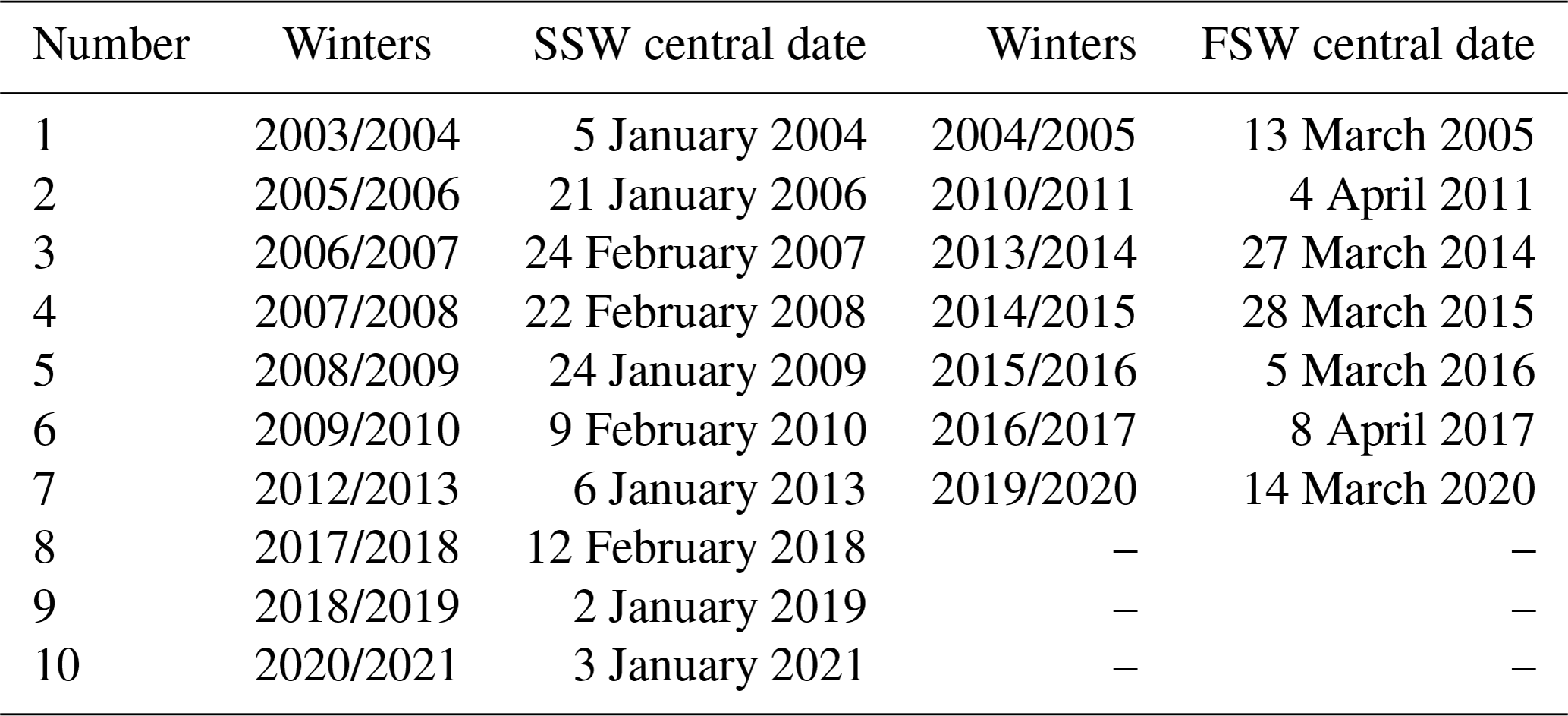
Stratospheric warming events are a crucial stratospheric phenomenon and indicate the vertical coupling of the entire middle atmosphere affecting the mesosphere, stratosphere, and troposphere. Many studies combined temperature increases and wind reversals to detect major SSW events in midwinter (Charlton and Polvani, 2007; Hu et al., 2014; Butler et al., 2015; Butler and Gerber, 2018). One of the most often-used definitions of a major SSW event during wintertime (Charlton and Polvani, 2007) is that zonal-mean zonal winds at 60° N and the 10 hPa level reverse direction from westerly to easterly and that the zonal-mean temperature gradient between 60 and 90° N becomes positive. As shown in Table 1, we identify 10 major SSW events in this study as described in Li et al. (2023). For the FSW events, different studies have analyzed springtime stratospheric zonal winds using single pressure levels at varying latitudes and thresholds (Black and McDaniel, 2007; Byrne et al., 2017; Matthias et al., 2021) as well as multiple pressure levels (Hardiman et al., 2011). We found seven early FSW events (in Table 1) identified by Butler and Domeisen (2021) based on the criterion that the daily mean zonal-mean zonal winds at 60° N latitude and 10 hPa exhibit an easterly flow and remain so continuously for more than 10 consecutive days, as outlined by Butler and Gerber (2018). The SSW and FSW composites will be discussed for the wind and temperature fields and anomalies, which are defined as deviations from the daily seasonal climatology.
Table 1Dates of the major SSW and early FSW events used for the composite in this study.
To examine the ozone anomalies during late winter over the polar latitude station, we summarize some key dynamical quantities of SSW and FSW events. Figure 1 illustrates the pressure–time evolution of the SSW and FSW composite zonal-mean zonal wind (at 60° N) and temperature (70–90° N) in MERRA-2 reanalysis data. Below approximately 0.1 hPa, the westerly wind rapidly weakens – lags by 10 d – and then switches to an easterly wind after the SSW onset (lags by 0 d) at 10 hPa in Fig. 1a. The easterly wind returns after approximately 15 d at 10 hPa. After around 20 d of SSW onset, the wind at 0.1 hPa reverses direction to westerly with a maximum speed of 80 m s−1 and stays like this for at least 20 d. The temperature fields undergo alterations in conjunction with the wind field reversal. The SSW onset is characterized by the rapid warming in the stratosphere in Fig. 1c, indicating the rapid descent of the stratopause to lower altitudes. In Fig. 1b, the zonal-mean zonal wind at 60° N and 10 hPa during an FSW event is easterly with lags of 50 d until the early summer and does not reverse its direction to westerly. The wind reversal is accompanied by a temperature increase exceeding 280 K after the FSW onset in Fig. 1d. Temperatures in the lower stratosphere also increase greatly, but there is cooling in the upper mesosphere.
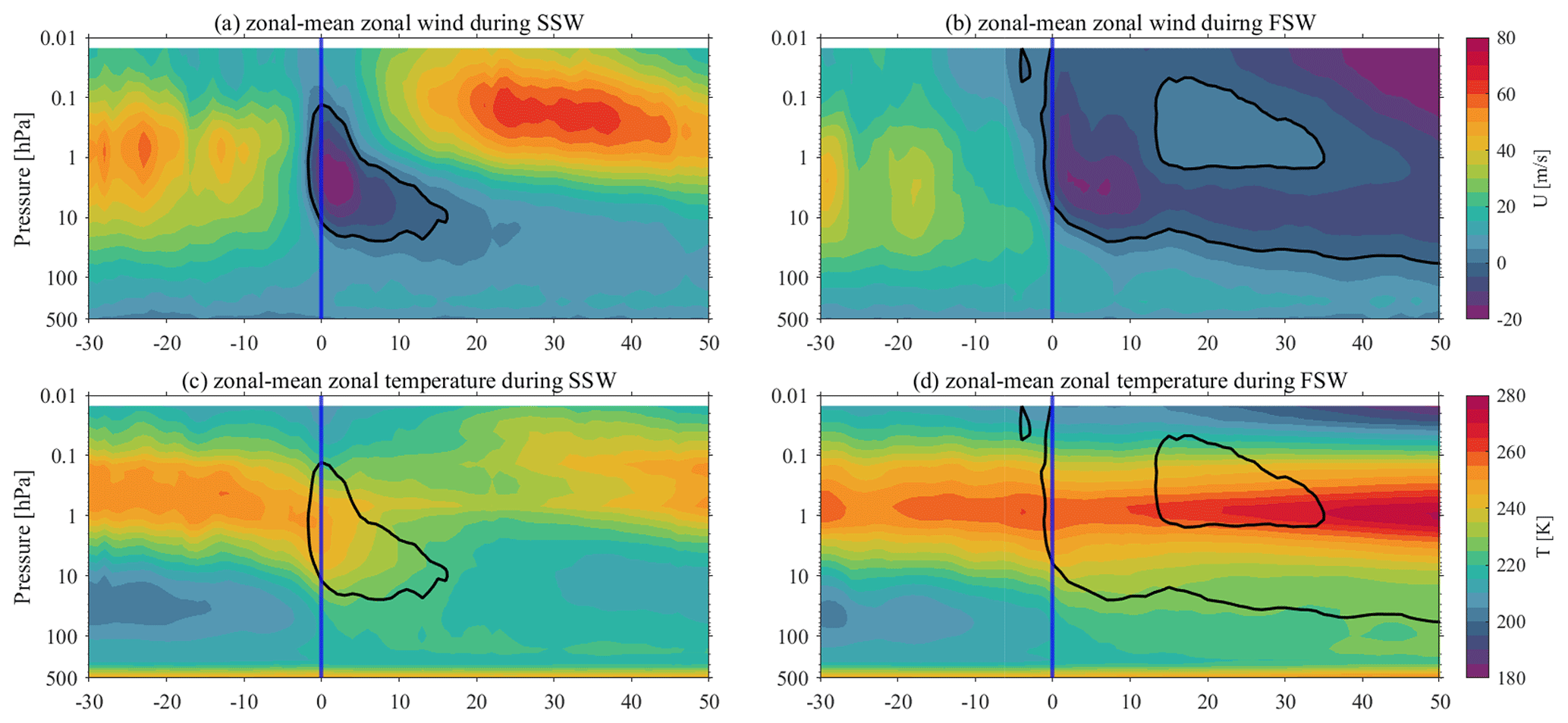
Figure 1Pressure–time section of the SSW and FSW composite zonal-mean (a, b) zonal wind and (c, d) temperature from MERRA-2. Time is relative to the SSW and FSW onset on the abscissa. The vertical blue line represents the onset day (day 0). The zero-wind contour is in black.
Furthermore, we derive anomalies for the relevant physical quantities by subtracting the mean climatology obtained from all years for our composites of SSW and FSW events. Significant anomalies of wind, temperature, and extend over nearly the entire pressure range and throughout the life cycle of SSW and FSW as shown in Fig. 2. The strongest negative wind anomalies occur during the first 15 d after the SSW onset and diminish within 20 d in the stratosphere, corresponding to the strongest positive anomalies in the mesosphere occurring between 20 and 50 d after the onset day as shown in Fig. 2a. These changes occur in parallel to rapid stratospheric warming, with the temperature maxima appearing in near-vertical quadrature with the wind anomalies during those 5 d before and after the SSW onset (Fig. 2c). During the recovery phase following the SSW, progressively descending negative anomalies in the stratosphere appear with positive anomalies in the mesosphere, along with the reformation of the “normal” stratopause. The lower mesosphere exhibits negative wind anomalies with lags ranging from −30 to 20 d, with the most pronounced negative values observed at 1 hPa (Fig. 2a). The vertical extent of the zonal wind and temperature anomalies at FSW onset is similar to that of the SSW event, but the magnitude and strength are different. The temperature anomaly at 1 hPa almost vanishes and remains around zero after FSW onset. anomalies over the polar regions (70–90° N) as an indicator of wave forcing show more intense downward propagation (blue) and upward propagation (red) during both events. The obvious difference between the two types of events is that strong upwelling starts about 3 weeks earlier at negative lags for SSW events (Fig. 2e). The statistically significant positive anomalies vanish after 15 d, giving way to negative anomalies emerging within 30 d in Fig. 2e. In contrast, FSW events exhibit anomalies that remain positive for a duration near 40 d above 1 hPa (Fig. 2f). The lasting anomalies after the FSWs at and below 1 hPa are very small though.
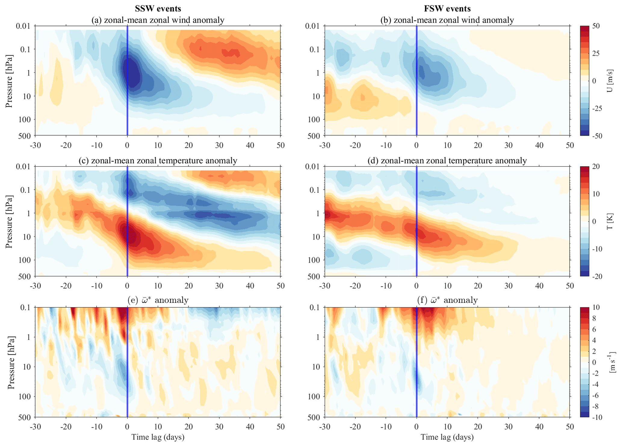
Figure 2Pressure–time section of the SSW and FSW composite zonal-mean (a, b) zonal wind anomalies, (c, d) temperature anomalies, and (e, f) vertical component of the residual circulation anomalies for the averaged polar regions (70–90° N) from MERRA-2.
Leveraging continuous ozone measurements from the ground-based radiometer GROMOS-C at Ny-Ålesund, Svalbard (79° N, 12° E), and combining MERRA-2 and MLS datasets, we analyze the temporal evolution of ozone and provide more details on the impacts of SSW and FSW events. The main benefit of the ground-based observations is the much higher temporal resolution of 2 h, which permits us to estimate the sampling bias from the MLS satellite, taking data at only two local times. This higher temporal resolution is also sufficient to resolve the daily ozone cycle (Schranz et al., 2018). Figure 3 exhibits the SSW and FSW composite ozone VMR at Ny-Ålesund (79° N, 12° E) as a function of the time lag for an event's central date. The GROMOS-C-measured ozone VMR over Ny-Ålesund is greatly enhanced after an SSW and FSW onset. The results indicate good agreement between MERRA-2 (below 0.1 hPa) and MLS with GROMOS-C observations. However, due to the complexity of altered dynamics in the winter polar regions introducing additional uncertainties into numerical models and data assimilation systems (Wargan et al., 2017), ozone VMRs exhibit dramatic variability (in Fig. 3c, d) in the mesosphere from MERRA-2. Discontinuities in MERRA-2 ozone (Shi et al., 2023) in the mesosphere (0.1–0.01 hPa) have to be taken into account, which is likely associated with the extension of stratospheric chemistry up to the mesosphere. Knowland et al. (2022) discussed the model ozone biases in MERRA-2 due to mesospheric parameterization being disabled in the NASA Goddard Earth Observing System Composition Forecast (GEOS-CF), and the stratospheric chemistry now extends up through the top of the GEOS atmosphere, thus avoiding the need to repeatedly read in production and loss rates. Gelaro et al. (2017) investigated these partially understandable increased deviations using the implemented radiative transfer schemes and other model physics such as interactive chemistry, which is computationally much more expensive. Shi et al. (2023) discussed the climatological deviations of the measurements from the ground-based radiometer GROMOS-C with MERRA-2 and MLS. Otherwise, the presence of much more atomic oxygen compared to ozone in the upper mesosphere could be used to explain the observed large discrepancies above 0.1 hPa when MERRA-2 ozone is compared with MLS and GROMOS-C. Our analysis reveals qualitative agreement in stratospheric ozone between MERRA-2 and observations from the GROMOS-C and MLS instruments during FSW and SSW events. This agreement serves as a robust justification for employing MERRA-2 data to explore the dynamics–chemistry relationship in subsequent steps of our research, providing confidence in the reliability of MERRA-2 ozone data for our analytical purposes.
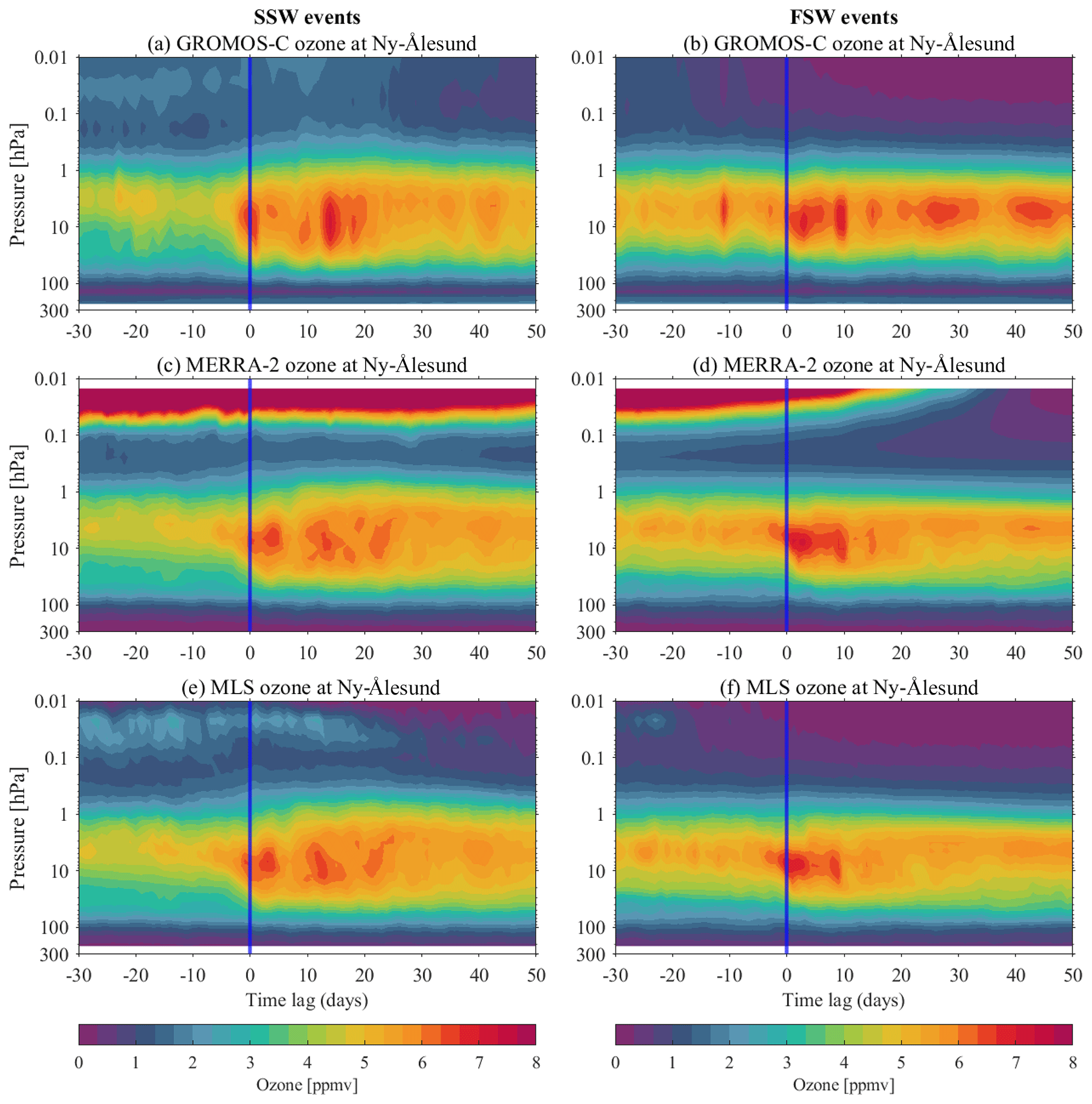
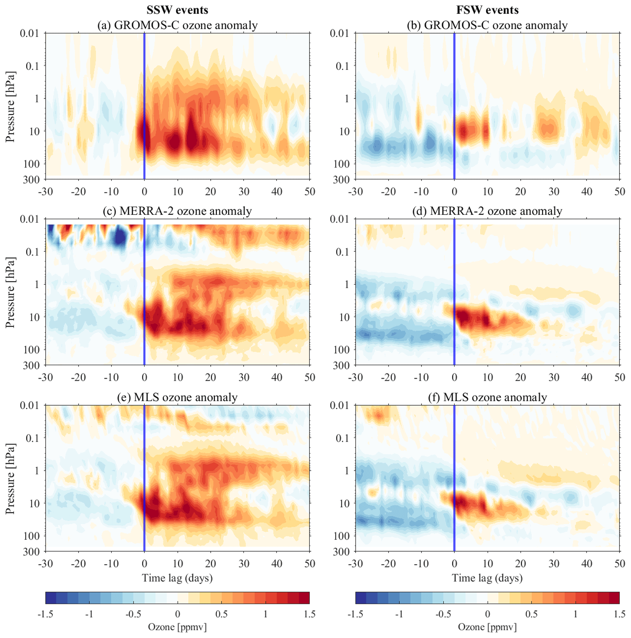
Figure 3Pressure–time section of SSW and FSW composite ozone VMR from (a, d) GROMOS-C, (b, e) MERRA-2, and (c, f) MLS at Ny-Ålesund (79° N, 12° E).
Figure 4 shows the composite ozone anomalies in GROMOS-C, MERRA-2, and MLS at Ny-Ålesund (79° N, 12° E) as a function of time lag for the SSW and FSW central date. These subplots show very similar behavior despite the variety of datasets and years covered. The strongest positive ozone anomalies of up to 1 ppmv for more than 30 consecutive days after SSW onset in the middle- and upper-stratospheric layers are evident. The positive ozone anomalies persist around 20 d after FSW onset in the middle stratosphere following a negative value of around 0.6 ppmv descending in the upper stratosphere. Otherwise, there is a negative ozone anomaly in the lower stratosphere and upper stratosphere before FSW onset that is stronger than before the onset of the SSW events. Note that the GROMOS-C composite is based on only three SSW and FSW events because the measurement campaign started in September 2015. The anomalies are estimated in terms of the daily climatology (between 2015 and 2022).
5.1 Seasonal cycle of the ozone transport budget
Seasonal changes in ozone tendencies from the eddy effect, advection transport, and chemical loss and production processes based on MERRA-2 reanalysis data for the period 2004–2021 are shown in Fig. 5. The contribution from each term in Eq. (2) is calculated to infer the seasonal cycle of the ozone transport budget in MERRA-2 averaged between 70 and 90° N. The ozone tendency shows a distinct increase during winter and fall and a decrease during spring and early summer. In Fig. 5b, the horizontal eddy transport exhibits a prominent seasonal cycle, with positive and significantly stronger ozone eddy mixing observed throughout the stratosphere over the entire year, except for the summer months. Vertical eddy transport tends to show a dipole pattern with opposite effects between the middle and upper stratosphere from late fall to early spring in Fig. 5c. This indicates that seasonality in eddy mixing plays a major role in the polar ozone annual cycle. Horizontal advection of ozone is much smaller compared to eddy-mixing and chemical processes as shown in Fig. 5d (an increase of 5 times). However, it has negative effects on the ozone mixing transport in the polar regions. During fall and winter, the vertical advection transport exhibits a pattern comparable to that of the vertical eddy term, yet it demonstrates a tendency towards positive values in the upper stratosphere during summer. Finally, the chemical term is positive during winter in the middle stratosphere. However, the greatest ozone destruction occurs in spring, reaching its maximum in April.
Figure 5g–i show the seasonal cycle of all terms averaged over the latitudes from 70 to 90° N for the pressure levels 10 hPa (∼ 30 km), 3 hPa K (∼ 40 km), and 1 hPa (∼ 50 km). At 10 hPa horizontal eddy transport and net chemical loss nearly balance each other out, particularly from February to June. Vertical eddy transport makes a negative contribution from September to April. Horizontal eddy transport has a large positive contribution of within 0.4 ppmv d−1 in March at 3 hPa, corresponding to maximum chemical ozone destruction. However, chemical production starts from October to February and has a peak in January at 3 hPa. Thus, the shape of the ozone seasonal cycle is mainly determined by the seasonally varying eddy-mixing transport and chemical loss and production. At 1 hPa, the chemical term is of crucial relevance, and the seasonal budget of ozone is completely controlled by competing effects of horizontal eddy transport and chemical terms. As a result, the eddy mixing effectively transports ozone into the polar region during winter and spring, where the horizontal eddy transport is so large that it balances a large fraction of the chemical ozone destruction.
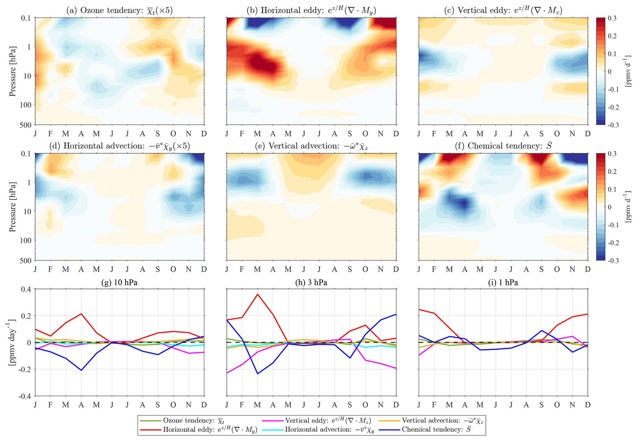
Figure 5Seasonal cycle of the ozone tendencies as a function of time and pressure from MERRA-2 (period 2004–2021): (a) ozone tendency , (b) horizontal eddy transport , (c) vertical eddy transport , (d) horizontal advection transport , (e) vertical advection transport , and (f) chemical loss and production averaged over the polar regions (70–90° N) based on Eq. (2). The third row is the comparison of each term at different pressure levels: (g) 10 hPa, (h) 3 hPa, and (i) 1 hPa.
Although the chemical term displays the features of a chemical sink and source term, including location and seasonality in Fig. 5, there are differences compared to other methods of calculating ozone loss rates as shown in Fig. 6. We use the output from the chemistry transport model to display the seasonal cycle of TOT, DYN, and CHM based on Eq. (1). TOT shows good agreement in magnitude with the results from the TEM analysis. The largest discrepancy between and CHM (between DYN and CHM) occurs during the winter months in the middle and upper stratosphere, where the negative (positive) tendency in Eq. (2) is found rather than the positive (negative) tendency found in Eq. (1). It is important to note that the residual term in the TEM equation is shown to be representative of the chemical net production term (≈ ). This is an approximation since it also contains ozone transport due to unresolved waves, such as gravity waves (Plumb, 2002). One of the causes of this discrepancy is that calculations for MERRA-2 rely on the dynamical diagnostic terms in Eq. (2), in particular the effects of irreversible eddy-mixing transport . The horizontal eddy mixing is predominantly influenced by the forcing from the breaking of resolved waves (Plumb, 2002). Furthermore, this discrepancy is very pronounced during winter, as shown in Figs. 5f and 6c. Randel et al. (1994) and Minganti et al. (2020) studied the effect of the SSW event on the N2O TEM budget, which showed more contributions of vertical advection and horizontal eddy mixing to this budget during the SSW event than in the seasonal mean. Thus, we can explain the resulting discrepancy in the ozone TEM budget from the highly frequent occurrence of SSW events in the Northern Hemisphere, which affects the seasonal cycle in climatology in the polar regions. Hence, the discrepancy in the ozone TEM budget can be accounted for by the more frequent occurrence of midwinter SSW events in the Northern Hemisphere, leading to the effects on the ozone TEM budget in the polar regions at the seasonal scale. Determining the ozone transport mechanisms during stratospheric extreme events for better understanding of stratospheric processes and ozone variability in stratospheric chemistry–climate models and better representation in chemistry–climate models therefore has the potential to improve medium-range weather forecasts during high-latitude winter.
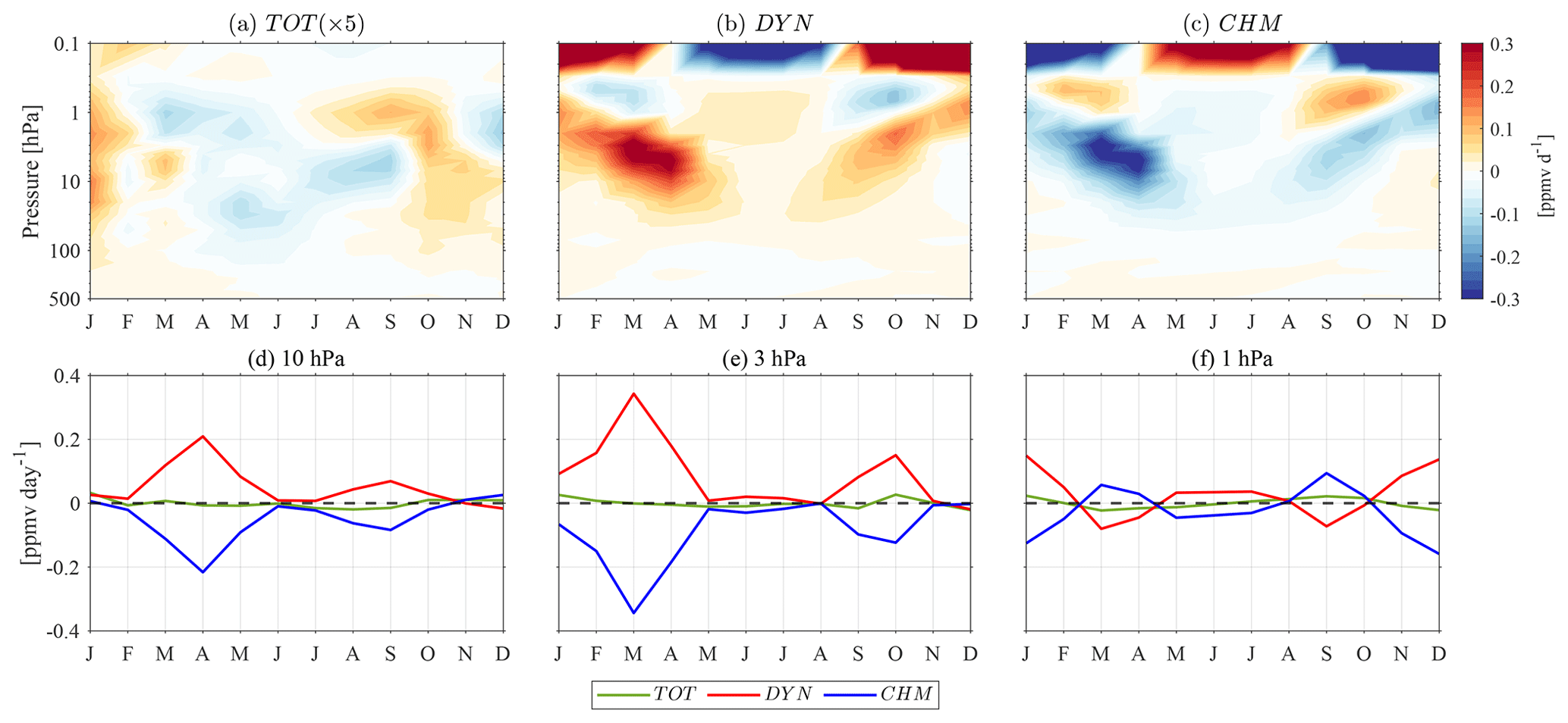
Figure 6Seasonal cycle of (a) TOT, (b) the ozone tendency anomaly due to dynamics, and (c) the parameterized chemistry averaged over the polar regions (70–90° N) based on Eq. (1). The second row is the comparison of each term at different pressure levels: (d) 10 hPa, (e) 3 hPa, and (f) 1 hPa.
5.2 Insights into the ozone budget during SSW and FSW events
A climatological comparison of ozone anomalies throughout the life cycle of SSW and FSW events using MERRA-2 and MLS data provides more details about the dynamical and chemical contributions and temporal evolution of both events. Figure 7 visualizes the composite vertical structure and evolution of ozone anomalies in MERRA-2 and MLS during SSW and FSW events averaged over the polar regions (70–90° N). The vertically resolved ozone VMR (Fig. 7a, c) shows a more complicated picture during SSW events compared to FSW events (Fig. 7b, d). A weak negative ozone anomaly in the lower and middle stratosphere and a positive ozone anomaly in the upper stratosphere close to the SSW onset are presumably related to the polar stratosphere being dominated by an anomalously strong and cold vortex during this time, leading to reduced transport of ozone-rich air masses into the polar regions. Within the first 20 d following the SSW onset, the ozone VMR anomalies rapidly increase by more than 1 ppmv and persist for up to 50 d until late winter in the middle stratosphere (30–10 hPa). The negative anomalies above 5 hPa exist only briefly at the SSW onset. They are followed by persistent positive anomalies, which tend to reach their maximum value with lags of 20 d in the stratopause and lower mesosphere. During FSW events the ozone anomaly is unusually negative below the 10 hPa level before the onset day, exhibiting a reduced ozone VMR of about −0.8 ppmv from lags of −30 to 0 d compared to the climatology. Above 5 hPa, the negative anomalies persist over the life cycle of FSW events and the altitude of the negative anomaly tends to descend with time after the FSW onset. However, the positive ozone anomalies have a peak in the middle stratosphere at the FSW onset and also persist for about 20 d, propagating downward into the lower stratosphere. The structure of these anomalies differs somewhat from that of SSW events, particularly in the transition from rapidly increasing positive to descending negative anomaly tendencies in the middle to upper stratosphere after FSW onset.
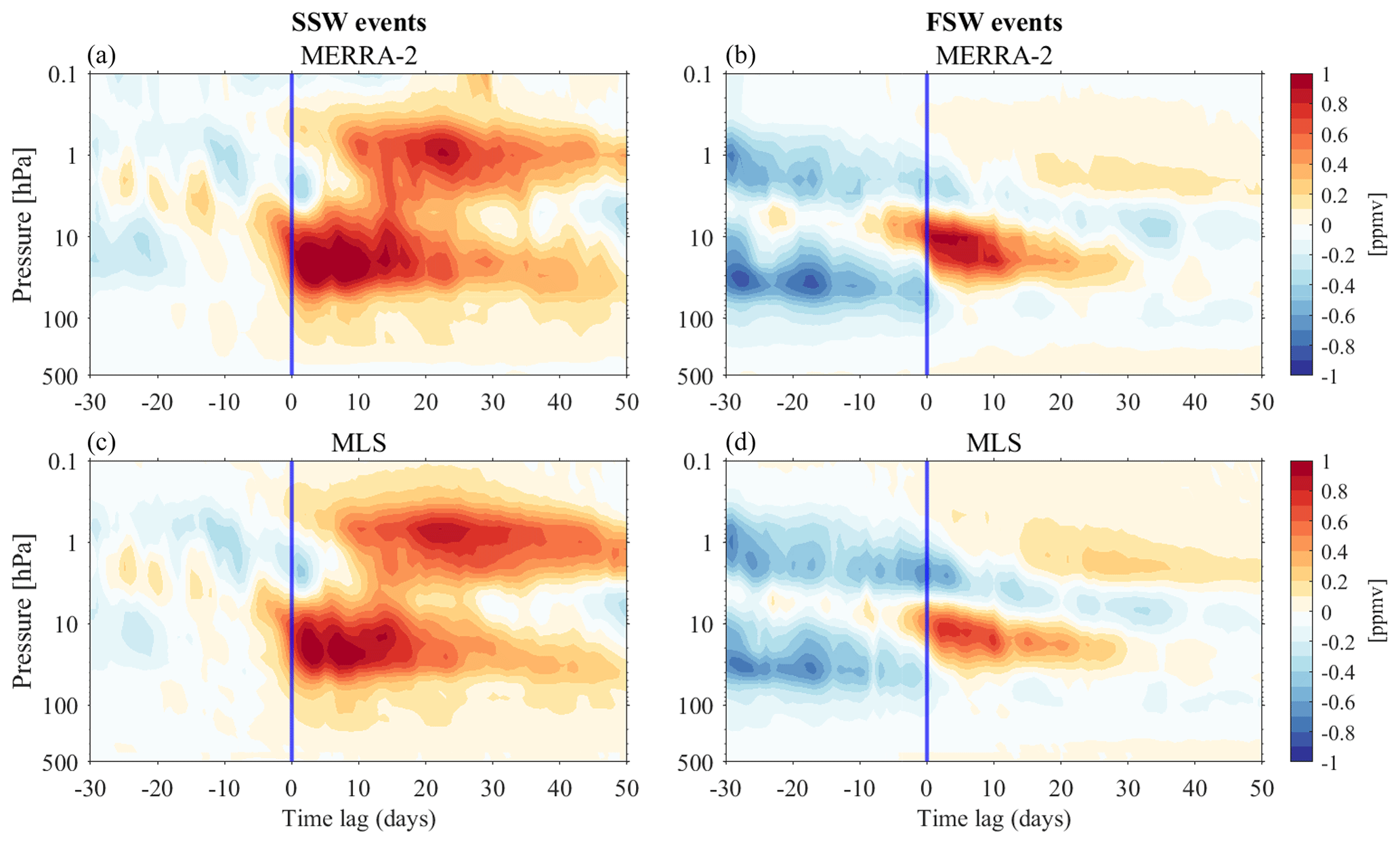
Figure 7Evolution of the ozone anomalies for the composite of SSW and FSW events as a function of time and pressure averaged over the polar regions (70–90° N) for (a, b) MERRA-2 and (c, d) MLS.
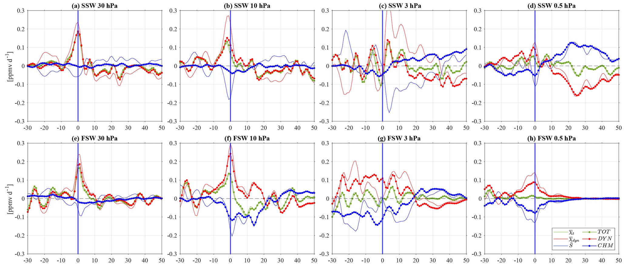
Utilizing the results obtained from vertically integrated ozone tendency and ozone continuity equations, we compare the specific contributions of dynamical and chemical processes to the observed ozone anomaly behavior during SSWs and FSWs. Figures 8 and 9 present the anomalous ozone tendencies averaged between 70 and 90° N during SSW and FSW events, along with their associated dynamical and chemical fields. We have omitted the contributions due to the horizontal advection (not shown) since they are small compared to the other processes. Moreover, we decompose the total ozone tendency into contributions of dynamical and chemical terms in Eq. (1) to infer the sources of transient changes in the polar stratospheric ozone tendency anomalies.
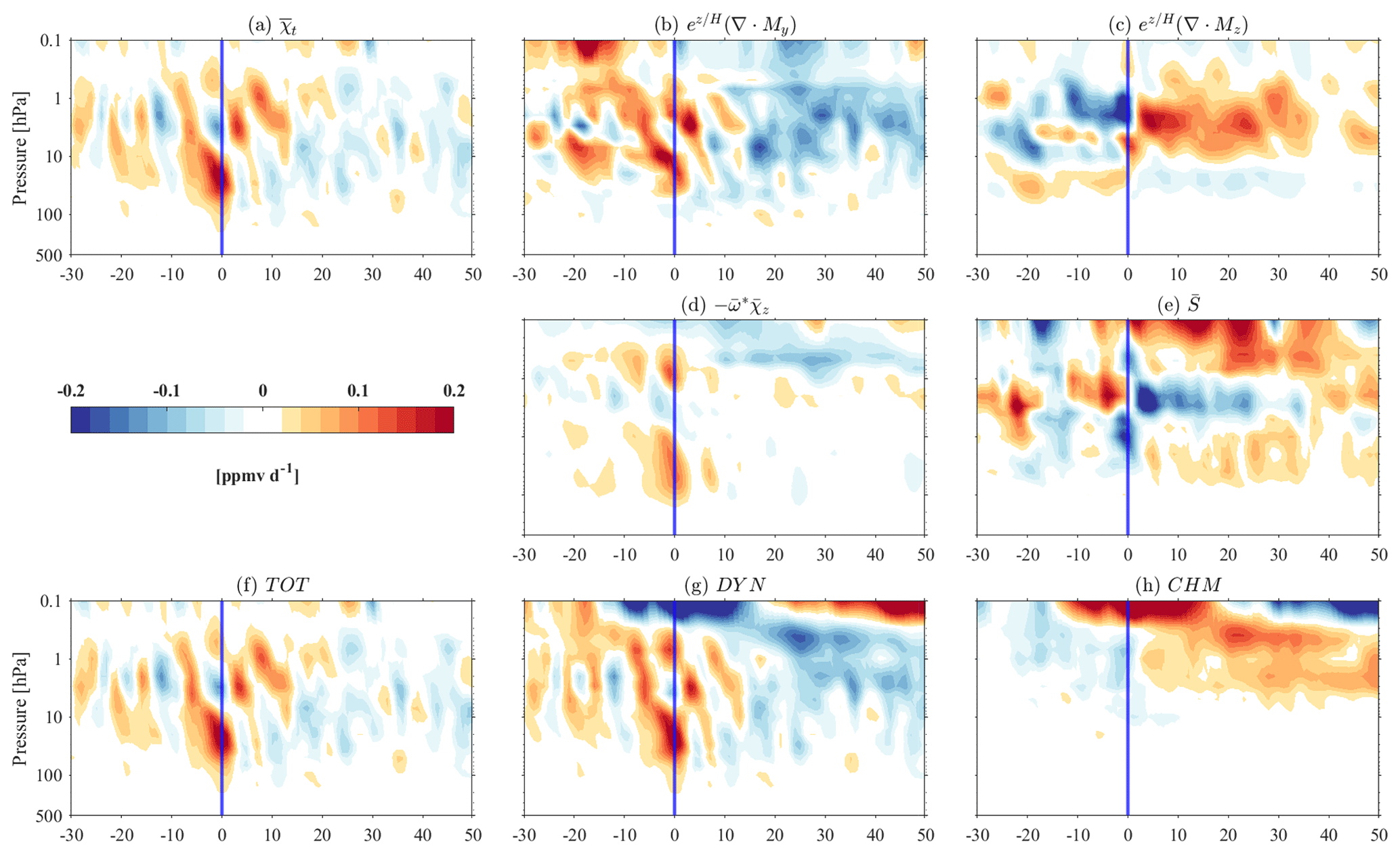
Figure 8Anomalous ozone tendencies for SSW events as a function of time and pressure averaged over the polar regions (70–90° N) from MERRA-2: calculation of the (a) ozone tendency anomaly due to the dynamical field that is decomposed into the (b) horizontal eddy transport effect , (c) vertical eddy transport effect , (d) vertical advection transport , and (e) chemical net chemical field based on Eq. (2). The third row shows (f) the TOT, (g) the ozone tendency anomaly due to dynamics (DYN), and (h) the parameterized chemistry (CHM) based on Eq. (1).
The results indicate pronounced ozone tendency anomalies primarily between 100 and 10 hPa, starting with a positive ozone tendency anomaly from lag −8 d to the onset day (Fig. 8a). The evolution of the ozone tendency anomaly is consistent with the TOT anomaly in Fig. 8f. The evolution of the TOT anomaly in the lower and middle stratosphere (between 100 and 1 hPa) is mainly dominated by DYN (Fig. 8g). DYN in the lower and middle stratosphere (100 and 10 hPa) is primarily attributed to the ozone transport via vertical advection (Fig. 8d) and eddy transport effects (Fig. 8b, c). Notably, the dominance of the dynamical term in or the TOT anomaly in the lower stratosphere during the life cycle of the SSW composite is consistent with the transient changes in vertical residual mean transport (Fig. 2). A strong negative exists in the polar regions corresponding to the positive and TOT (Fig. A1). An intensified residual circulation significantly weakens or breaks up the polar vortex, hence facilitating poleward ozone transport and resulting in an increase in the ozone VMR (Schranz et al., 2020; Shi et al., 2023; Bahramvash Shams et al., 2022; Harzer et al., 2023).
In the upper stratosphere, there is a notable negative ozone tendency anomaly at the onset of SSW, primarily driven by horizontal eddy and vertical advection. The vertical eddy effect contributes to building up the negative ozone tendency anomaly, while the chemistry term tends to compensate for the ozone tendency anomaly from lag −10 d to the SSW onset day. Conversely, as the vertical eddy effect builds up the ozone tendency anomaly, the chemistry term balances or weakens the ozone tendency anomaly after the SSW onset. Positive vertical eddy transport and negative in the upper stratosphere (between 3 and 1 hPa) from SSW onset day 0 to lag 35 d partially counteract the dynamically induced ozone anomalies through (Fig. 8e). Interestingly, Fig. 8h presents two opposite attributions of CHM before and after SSW onset (the period is from lag −15 to 35 d) in the upper stratosphere, which is almost the opposite tendency compared with . The significant discrepancy during SSW events is evident in , with negative contributions in the upper stratosphere (Fig. A2) that are possibly due to uncertainties in calculating the eddy transport term, along with uncertainties in the rest of the dynamical terms. A potential source of discrepancy is that Eq. (2) does not account for the effects of numerical diffusion and vertical diffusion due to the gravity wave parameterization in particular; these are presumably non-negligible in the middle to upper stratosphere. As discussed in Brasseur and Solomon (2005), the polar middle stratosphere, as the transition layer, is intricate and requires consideration of various conditions and additional constraints. This is because ozone is chemically controlled above this layer, while below it is dynamically controlled.
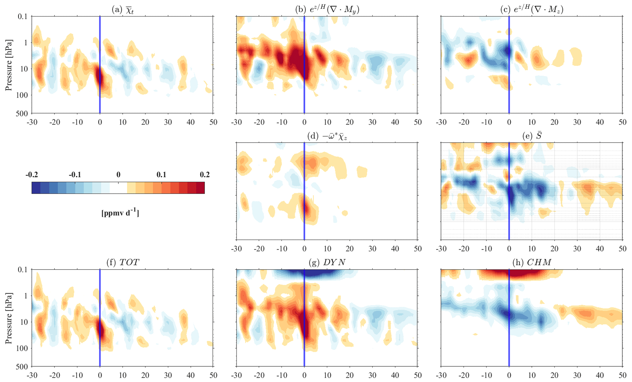
During FSW, the anomalous ozone tendency exhibits notable differences compared to SSW events, particularly in the middle stratosphere, where the FSW ozone tendency is affected by chemical and dynamical process-induced wave–mean flow interactions. In Fig. 9, the negative anomaly lags from 5 to 15 d in the middle stratosphere, which are attributed to the photochemical effects, partially counteracted (Fig. 9e and h) the positive horizontal eddy transport (Fig. 9b). In the lower stratosphere, the strong anomalous positive tendency at FSW onset (Fig. 9a) is associated with the dynamical terms, which are horizontal eddy and enhanced vertical advection transports (Fig. 9b and d). In the upper stratosphere, there is no obvious ozone tendency anomaly at FSW onset, which can be explained by the negative contributions of vertical eddy transport (Fig. 9c) counteracted by other terms. The evolutions of TOT and are consistent with and CHM, respectively, in the lower and middle stratosphere (50–3 hPa) during FSW. In addition, the strong and CHM around FSW onset emphasize the importance of chemical processes in spring.
There is also remarkable agreement between and CHM (as well as between and DYN) anomalies in the lower mesosphere during the SSW and FSW events displayed in Fig. 8d, h. This can be attributed to the temperature–ozone relation that suggests that, in a region dominated by pure oxygen chemistry, a temperature decrease of 10 K would produce an increase in ozone of about 20 % (Brasseur and Solomon, 2005). Temperature changes will modify all temperature-dependent photochemical rates and hence feedback to the ozone chemistry. As shown in Fig. 1d and h, from lags of 10 to 40 d during SSW events in the lower mesosphere, the negative temperature anomaly is more than 10 K from of lags 10 to 40 d, and the positive ozone VMR anomaly reaches 0.5 ppmv. Ozone anomalies resulting from the negative dynamical transport and chemical production manifest a few days after SSW onset and last for an extended period of 50 d. During FSW events, positive dynamical transport and net chemical loss nearly balance each other out at 0.5 hPa (Fig. A2), leading ozone tendency anomalies to fluctuate around zero.
5.3 Dynamical control of the total column ozone
Many studies have highlighted the significant impact of enhanced propagation of planetary waves in the lower stratosphere on the increase in TCO in winter (Matthias et al., 2013; Shaw and Perlwitz, 2014; Lubis et al., 2017; Safieddine et al., 2020; Matthias et al., 2021), subsequently leading to reduced ozone depletion in springtime (Manney et al., 2020; Lawrence et al., 2020; Schranz et al., 2020). The positive TCO anomalies after SSW events span a period exceeding 40 d when analyzing data from ERA5 and MERRA-2 reanalysis, MLS, or comprehensive GCMs such as WACCM over the polar regions (de la Cámara et al., 2018b; Safieddine et al., 2020; Bahramvash Shams et al., 2022; Hocke et al., 2023). Robust positive TCO anomalies during early FSW events are influenced by the wave geometry of the FSW (Butler and Domeisen, 2021). Therefore, the dynamical behavior of SSW and FSW events which alter the chemical and dynamical evolution of the polar stratospheric ozone VMRs affects the distribution of TCO over the northern polar region. As TCO is dominated by the lower stratosphere, changes in lower-stratospheric ozone will map directly into TCO.
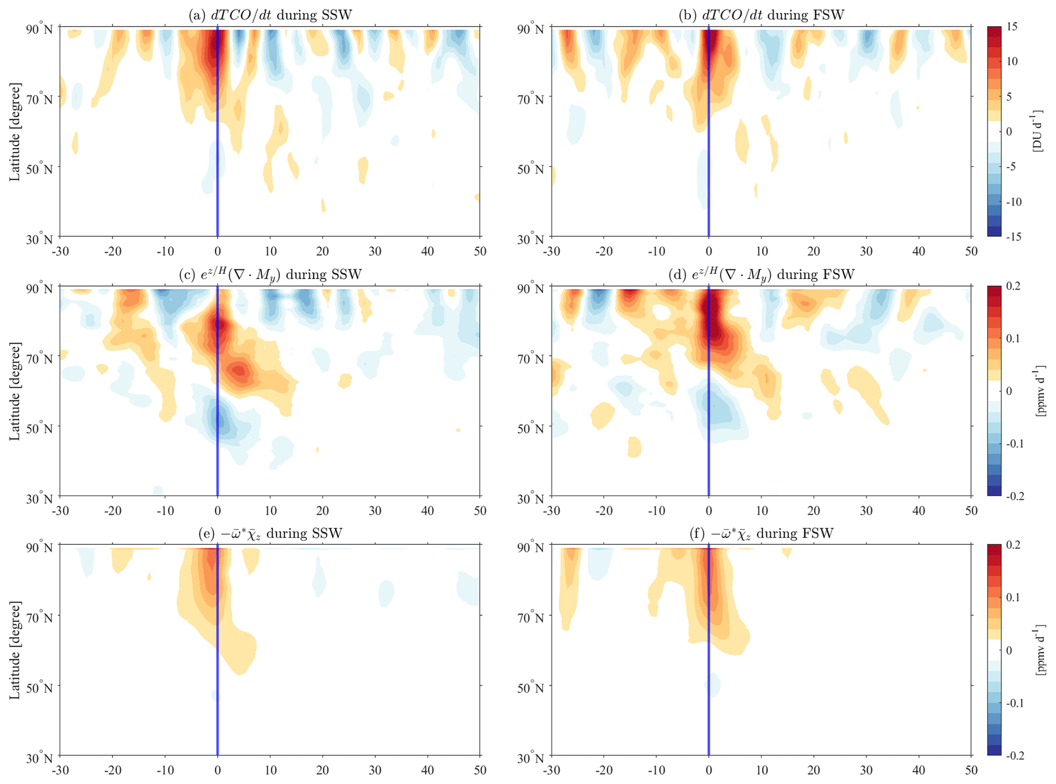
Quantitatively separating the effects of dynamic and chemical processes on TCO is challenging because polar ozone is similarly affected by each process. Therefore, we focus on the variability caused by dynamical processes in the TCO changes based on the relative contributions of dynamical and chemical processes in Sect. 5.2. We calculate TCO tendency anomalies in the Northern Hemisphere (30–90° N) during SSW and FSW events using MERRA-2 in Fig. 10. We find that enhanced polar TCO close to the SSW and FSW onset is mainly induced by the anomalous horizontal eddy effect and vertical advection transport in the lower stratosphere (at 30 hPa in Fig. 10). In terms of the 450 K level, it turns out that the dynamical processes involved affect the polar TCO tendency anomalies. Figures 10 and A3 indicate that the polar TCO anomalies during SSW and FSW events can be attributed to anomalous dynamical processes.
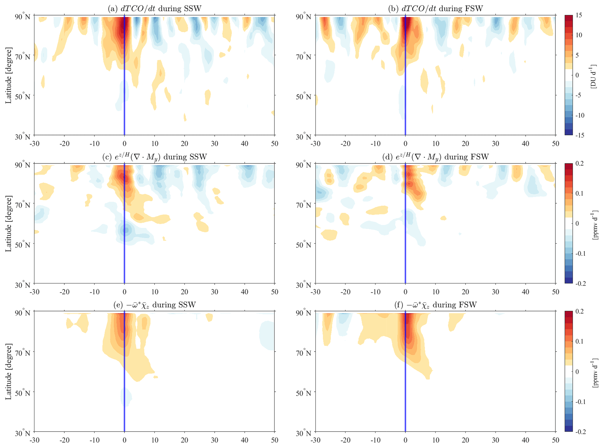
Figure 10Evolution of the TCO tendency anomalies (DU d−1), the horizontal eddy effect , and the vertical advection transport anomalies at 30 hPa (ppmv d−1) for the composite of SSW (a, c, e) and FSW (b, d, f) events as a function of time and latitude in the Northern Hemisphere.
In this paper, we use MERRA-2 reanalysis data to identify SSW and FSW events by analyzing zonal wind fields and polar temperatures covering the period from 2004 to 2022. We focused on investigating the vertically resolved polar ozone variations during both SSW and FSW events and quantifying their driving mechanisms. The impact of major SSW and early FSW events on ozone in the stratosphere and mesosphere was investigated using microwave radiometer measurements taken by GROMOS-C at Ny-Ålesund, Svalbard (79° N, 12° E). Microwave observations of the daily ozone profiles during SSW and FSW events were retrieved in the stratosphere and lower mesosphere at 20–70 km. GROMOS-C captured the high variability of middle-stratospheric ozone fluctuations, showing a dramatic increase in ozone VMRs after SSW and FSW onset. For validation purposes, local changes in ozone VMRs from MERRA-2 in the stratosphere and mesosphere displayed common features in GROMOS-C and MLS under SSW and FSW conditions. Ozone anomalies are identified throughout the stratosphere and lower mesosphere (from 100 to 0.1 hPa) during SSW and FSW events. Notably, positive ozone VMR anomalies of approximately 1.5 ppmv in the middle stratosphere persisting for 30 d after SSW onset and 20 d after FSW onset have been documented.
Qualitative agreement in ozone between MERRA-2 and observations from GROMOS-C and MLS during FSW and SSW events provides confidence in the reliability of MERRA-2 data up to an altitude corresponding to 0.1 hPa for investigating the driving mechanisms of polar ozone dynamics and chemistry. Above 0.1 hPa, MERRA-2 ozone data indicate larger deviations from GROMOS-C and MLS due to the used odd-oxygen family model. In the mesosphere, odd oxygen starts to be dominated by atomic oxygen and no longer by ozone and thus can explain why MERRA-2 exhibits less good agreement with the observations, although MLS ozone is assimilated up to 0.02 hPa in the mesosphere. Based on the TEM budget equation, we rationalize the impact of SSW and FSW events on ozone anomalies by calculating dynamical and chemical terms in Eq. (2) using meteorological variables provided by MERRA-2 reanalysis data.
-
The enhanced transport of ozone into the polar cap on the seasonal scale is attributed to the increased occurrence of SSW events during midwinter in the Northern Hemisphere. However, more ozone chemical loss in springtime than the climatology of the seasonal mean is attributed to more early FSW events (Matthias et al., 2021).
-
The impact of SSW and FSW events on total ozone tendency is shown by the altitude tendencies from the lower to middle stratosphere (from the middle to upper stratosphere and to the lower mesosphere) that change from positive to negative (from negative to positive) close to onset.
-
Positive ozone anomalies larger than 1 ppmv close to SSW onset in the lower and middle stratosphere are attributed to the dynamical processes of the horizontal eddy effect and vertical advection transport, while this response pattern for FSW events is associated with the combined effects of dynamical and chemical terms reflected by the photochemical effect counteracted partially by positive horizontal eddy transport, in particular in the middle stratosphere.
-
Substantial differences in the chemical fields in the upper stratosphere displaying negative and positive CHM after SSW onset within 30 d are attributed to greater uncertainties in TEM diagnostics, particularly when calculating eddy effects and mean advection transports.
Our results establish a new perspective on the driving mechanisms behind pronounced polar ozone anomalies associated with dynamical and chemical processes in the stratosphere during SSW and FSW events. Although previous studies have shown composite spatial and temporal ozone responses to SSW events in the Arctic (de la Cámara et al., 2018a, b; Hong and Reichler, 2021; Bahramvash Shams et al., 2022; Harzer et al., 2023), we took a more comprehensive approach and higher altitudes up to the lower mesosphere to study the polar ozone anomalies, and we considered not only major SSW events but also early FSW events. The polar ozone response pattern reflects the underlying ozone transport anomalies when viewed over the polar latitude station with a vertically resolved response structure. The ozone response signature during SSW and FSW events in the stratosphere and lower mesosphere can be explained by consecutive counteracting anomalous tendencies associated with eddy-mixing effects and advection transports on daily timescales, as well as chemical production and loss. In particular, these studies showed that weaker midwinter planetary wave forcing in the stratosphere due to weaker upward wave propagation leads to lower spring Arctic temperatures and thus to more ozone destruction in spring. In particular, our results suggest that anomalous ozone tendencies during FSW events in the middle stratosphere can be attributed to the dynamical field counteracted partially by chemical loss. Furthermore, the type of SSW is characterized by anomalous evolution of ozone tendencies in winter, leading to distinct chemistry patterns and variations in the intensity and duration of anomalous transport and mixing properties in the upper stratosphere. In contrast, chemistry contributions during years with FSW events in spring are relatively less pronounced in the upper stratosphere, representing a predominantly smooth transition according to the climatology.
Finally, referring back to a novel aspect of this study involving the relative contributions of dynamical and chemical effects to the anomalous ozone tendency, we found that a significant discrepancy in chemical effects between utilizing TEM diagnostics and CHM from chemistry transport models is observed during SSW events, which is not replicated in FSW events, as shown in Fig. 9e, h. This finding contributes to a growing body of evidence suggesting that the difference is associated with substantial uncertainties in the calculated dynamical terms derived from the MERRA-2 reanalysis for SSW events. However, it is unclear whether the remaining differences only result from the quality of the reanalysis data and substantial anthropogenic ozone-depleting substances in recent decades, indicating that ozone chemistry has become increasingly important in governing climate variability. There have been several studies showing that polar vortex dynamics are key to understanding polar ozone VMRs (Sun et al., 2014; Banerjee et al., 2020; Schranz et al., 2020; Shi et al., 2023). Due to the ban on chlorofluorocarbons (CFCs) that the Montreal Protocol ozone depletion policy was supposed to enforce, a trend reversal in the circulation is expected. Recent studies show such a trend reversal; however, it has not yet been confirmed whether the ozone recovery or the increased carbon dioxide is the cause of the changes in dynamics. Monitoring ozone in the stratosphere and lower mesosphere therefore remains a high priority and is supported by the Global Atmospheric Watch (GAW) program. In addition, we found that the ozone tendency in the lower stratosphere is primarily due to the horizontal eddy effect and vertical advection transport. Thus, we consider the observed variability in zonally averaged TCO in the polar regions for SSW and FSW events from MERRA-2. Dynamical processes in the lower stratosphere dominate TCO variability.
In general, the findings of this study contribute to a more comprehensive interpretation of the observed ozone variability at polar stations, with particular emphasis on the ozone anomaly situation. While existing research has predominantly concentrated on dynamic effects on Arctic ozone (de la Cámara et al., 2018b; Bahramvash Shams et al., 2022; Harzer et al., 2023), our study emphasizes the combined contribution of dynamical and chemical effects to polar ozone anomalies. This is especially evident because the anomalies of polar TCO during SSW and FSW events can be attributed to wave-driven anomalous dynamics. Therefore, understanding the interplay between dynamical and chemical processes during stratospheric extreme events will enhance our comprehension of the connections between middle- and upper-stratospheric dynamics and ozone chemistry. This knowledge is crucial for interpreting the observed vertically resolved pattern of daily variability and better quantifying polar ozone evolution.
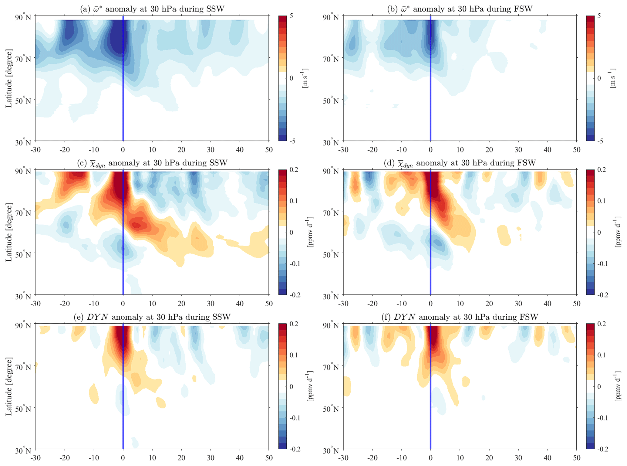
Figure A1Evolution of the anomalies (m s−1) and as well as the DYN anomalies at 30 hPa (ppmv d−1) for the composite of SSW (a, c, e) and FSW (b, d, f) events as a function of time and latitude in the Northern Hemisphere.
The GROMOS-C level-2 data are provided by the Network for the Detection of Atmospheric Composition Change (NDACC) and are available at the NDACC data repository https://www-air.larc.nasa.gov/pub/NDACC/PUBLIC/meta/mwave/ (University of Bern, 2024). The MLS v5 data are available from the NASA Goddard Space Flight Center Earth Sciences Data and Information Services Center (GES DISC) at https://doi.org/10.5067/Aura/MLS/DATA2516 (Schwartz et al., 2020). The MERRA-2 data are provided by NASA at the Modeling and Assimilation Data and Information Services Center (MDISC) and are available at the model level (Global Modeling and Assimilation Office, 2015b) at https://doi.org/10.5067/WWQSXQ8IVFW8, at the pressure level (Global Modeling and Assimilation Office, 2015a) at https://doi.org/10.5067/QBZ6MG944HW0, and for ozone tendency (Global Modeling and Assimilation Office, 2015c) at https://doi.org/10.5067/S0LYTK57786Z.
GSh was responsible for the ground-based ozone measurements with GROMOS-C, performed the data analysis, and prepared the manuscript. ES provided the Aura MLS data. WK helped with the data analysis. GSt designed the concept of the study and contributed to the interpretation of the results. All of the authors discussed the scientific findings and provided valuable feedback for manuscript editing.
The contact author has declared that none of the authors has any competing interests.
Publisher’s note: Copernicus Publications remains neutral with regard to jurisdictional claims made in the text, published maps, institutional affiliations, or any other geographical representation in this paper. While Copernicus Publications makes every effort to include appropriate place names, the final responsibility lies with the authors.
Guochun Shi, Gunter Stober, and Witali Krochin are members of the Oeschger Center for Climate Change Research. The authors acknowledge NASA's GMAO for providing the MERRA-2 reanalysis data and the Aura MLS team for providing the satellite data. Finally, we thank the two reviewers and the editors for the very helpful comments and suggestions.
This research has been supported by the Swiss National Science Foundation (grant no. 200021-200517/1).
This paper was edited by Jianzhong Ma and reviewed by three anonymous referees.
Albers, J. R. and Birner, T.: Vortex preconditioning due to planetary and gravity waves prior to sudden stratospheric warmings, J. Atmos. Sci., 71, 4028–4054, 2014. a
Albers, J. R., Perlwitz, J., Butler, A. H., Birner, T., Kiladis, G. N., Lawrence, Z. D., Manney, G. L., Langford, A. O., and Dias, J.: Mechanisms governing interannual variability of stratosphere-to-troposphere ozone transport, J. Geophys. Res.-Atmos., 123, 234–260, https://doi.org/10.5194/acp-20-12609-2020, 2018. a
Andrews, D., Holton, J., and Leovy, C.: Middle Atmosphere Dynamics, International Geophysics, Elsevier Science, ISBN 9780120585762, https://books.google.de/books?id=N1oNurYZefAC (last access: 21 July 2016), 1987. a, b, c
Bahramvash Shams, S., Walden, V. P., Hannigan, J. W., Randel, W. J., Petropavlovskikh, I. V., Butler, A. H., and de la Cámara, A.: Analyzing ozone variations and uncertainties at high latitudes during sudden stratospheric warming events using MERRA-2, Atmos. Chem. Phys., 22, 5435–5458, https://doi.org/10.5194/acp-22-5435-2022, 2022. a, b, c, d, e, f
Baldwin, M. P., Ayarzagüena, B., Birner, T., Butchart, N., Butler, A. H., Charlton-Perez, A. J., Domeisen, D. I., Garfinkel, C. I., Garny, H., Gerber, E. P., Hegglin, M. I., Langematz, U., and Pedatella, N. M.: Sudden stratospheric warmings, Rev. Geophys., 59, e2020RG000708, https://doi.org/10.1029/2020RG000708, 2021. a
Banerjee, A., Fyfe, J. C., Polvani, L. M., Waugh, D., and Chang, K.-L.: A pause in Southern Hemisphere circulation trends due to the Montreal Protocol, Nature, 579, 544–548, 2020. a
Black, R. X. and McDaniel, B. A.: Interannual variability in the Southern Hemisphere circulation organized by stratospheric final warming events, J. Atmos. Sci., 64, 2968–2974, 2007. a, b
Bosilovich, M. G., Akella, S., Coy, L., Cullather, R., Draper, C., Gelaro, R., Kovach, R., Liu, Q., Molod, A., Norris, P., Wargan, K., Chao, W., Reichle, R., Takacs, L., Vikhliaev, Y., Bloom, S., Collow, A., Firth, S., Labows, G., Partyka, G., Pawson, S., Reale, O., Schubert, S. D., and Suarez, M.: MERRA-2: Initial Evaluation of the Climate. Technical Report Series on Global Modeling and Data Assimilation, Tech. Rep. NASA/TM-2015-104606, https://gmao.gsfc.nasa.gov/pubs/docs/Bosilovich785.pdf (last access: 12 July 2016), 2015. a, b, c
Brasseur, G. and Solomon, S.: Aeronomy of the Middle Atmosphere: Chemistry and Physics of the Stratosphere and Mesosphere, in: Atmospheric and Oceanographic Sciences Library, Springer Netherlands, 2005. a, b
Butler, A. H. and Domeisen, D. I. V.: The wave geometry of final stratospheric warming events, Weather Clim. Dynam., 2, 453–474, https://doi.org/10.5194/wcd-2-453-2021, 2021. a, b
Butler, A. H. and Gerber, E. P.: Optimizing the Definition of a Sudden Stratospheric Warming, J. Climate, 31, 2337–2344, https://doi.org/10.1175/JCLI-D-17-0648.1, 2018. a, b
Butler, A. H., Seidel, D. J., Hardiman, S. C., Butchart, N., Birner, T., and Match, A.: Defining Sudden Stratospheric Warmings, B. Am. Meteorol. Soc., 96, 1913–1928, https://doi.org/10.1175/BAMS-D-13-00173.1, 2015. a, b
Byrne, N. J., Shepherd, T. G., Woollings, T., and Plumb, R. A.: Nonstationarity in Southern Hemisphere climate variability associated with the seasonal breakdown of the stratospheric polar vortex, J. Climate, 30, 7125–7139, 2017. a
Charlton, A. J. and Polvani, L. M.: A New Look at Stratospheric Sudden Warmings. Part I: Climatology and Modeling Benchmarks, J. Climate, 20, 449–469, https://doi.org/10.1175/JCLI3996.1, 2007. a, b, c
de la Cámara, A., Abalos, M., and Hitchcock, P.: Changes in stratospheric transport and mixing during sudden stratospheric warmings, J. Geophys. Res.-Atmos., 123, 3356–3373, 2018a. a
de la Cámara, A., Abalos, M., Hitchcock, P., Calvo, N., and Garcia, R. R.: Response of Arctic ozone to sudden stratospheric warmings, Atmos. Chem. Phys., 18, 16499–16513, https://doi.org/10.5194/acp-18-16499-2018, 2018b. a, b, c, d
Eriksson, P., Jiménez, C., and Buehler, S. A.: Qpack, a general tool for instrument simulation and retrieval work, J. Quant. Spectrosc. Ra., 91, 47–64, https://doi.org/10.1016/j.jqsrt.2004.05.050, 2005. a
Eriksson, P., Buehler, S., Davis, C., Emde, C., and Lemke, O.: ARTS, the atmospheric radiative transfer simulator, version 2, J. Quant. Spectrosc. Ra., 112, 1551–1558, https://doi.org/10.1016/j.jqsrt.2011.03.001, 2011. a
Fernandez, S., Murk, A., and Kämpfer, N.: GROMOS-C, a novel ground-based microwave radiometer for ozone measurement campaigns, Atmos. Meas. Tech., 8, 2649–2662, https://doi.org/10.5194/amt-8-2649-2015, 2015. a
Friedel, M., Chiodo, G., Stenke, A., Domeisen, D. I. V., and Peter, T.: Effects of Arctic ozone on the stratospheric spring onset and its surface impact, Atmos. Chem. Phys., 22, 13997–14017, https://doi.org/10.5194/acp-22-13997-2022, 2022. a, b
Gelaro, R., McCarty, W., Suárez, M. J., Todling, R., Molod, A., Takacs, L., Randles, C. A., Darmenov, A., Bosilovich, M. G., Reichle, R., Wargan, K., Coy, L., Cullather, R., Draper, C., Akella, S., Buchard, V., Conaty, A., da Silva, A. M., Gu, W., Kim, G.-K., Koster, R., Lucchesi, R., Merkova, D., Nielsen, J. E., Partyka, G., Pawson, S., Putman, W., Rienecker, M., Schubert, S. D., Sienkiewicz, M., and Zhao, B.: The modern-era retrospective analysis for research and applications, version 2 (MERRA-2), J. Climate, 30, 5419–5454, 2017. a, b, c, d
Global Modeling and Assimilation Office (GMAO): MERRA-2 inst3_3d_asm_Np: 3d,3-Hourly,Instantaneous,Pressure-Level,Assimilation,Assimilated Meteorological Fields V5.12.4, Goddard Earth Sciences Data and Information Services Center (GES DISC) [data set], Greenbelt, MD, USA, https://doi.org/10.5067/QBZ6MG944HW0, 2015a. a
Global Modeling and Assimilation Office (GMAO): MERRA-2 inst3_3d_asm_Nv: 3d,3-Hourly,Instantaneous,Model-Level,Assimilation,Assimilated Meteorological Fields V5.12.4, Goddard Earth Sciences Data and Information Services Center (GES DISC) [data set], Greenbelt, MD, USA, https://doi.org/10.5067/WWQSXQ8IVFW8, 2015b. a
Global Modeling and Assimilation Office (GMAO): MERRA-2 tavg3_3d_odt_Np: 3d,3-Hourly,Time-Averaged,Pressure-Level,Assimilation,Ozone Tendencies V5.12.4, Goddard Earth Sciences Data and Information Services Center (GES DISC) [data set], Greenbelt, MD, USA, https://doi.org/10.5067/S0LYTK57786Z, 2015c. a
Hardiman, S. C., Butchart, N., Charlton-Perez, A. J., Shaw, T. A., Akiyoshi, H., Baumgaertner, A., Bekki, S., Braesicke, P., Chipperfield, M., Dameris, M., Garcia, R. R., Michou, M., Pawson, S., Rozanov, E., and Shibata, K.: Improved predictability of the troposphere using stratospheric final warmings, J. Geophys. Res.-Atmos., 116, D18113, https://doi.org/10.1029/2011JD015914, 2011. a
Harzer, F., Garny, H., Ploeger, F., Bönisch, H., Hoor, P., and Birner, T.: On the pattern of interannual polar vortex–ozone co-variability during northern hemispheric winter, Atmos. Chem. Phys., 23, 10661–10675, https://doi.org/10.5194/acp-23-10661-2023, 2023. a, b, c
Hocke, K., Sauvageat, E., and Bernet, L.: Response of Total Column Ozone at High Latitudes to Sudden Stratospheric Warmings, Atmosphere, 14, 450, https://doi.org/10.3390/atmos14030450, 2023. a
Holton, J. R.: The dynamics of sudden stratospheric warmings, Annu. Rev. Earth Pl. Sc., 8, 169–190, 1980. a
Hong, H.-J. and Reichler, T.: Local and remote response of ozone to Arctic stratospheric circulation extremes, Atmos. Chem. Phys., 21, 1159–1171, https://doi.org/10.5194/acp-21-1159-2021, 2021. a, b, c, d
Hu, J., Ren, R., and Xu, H.: Occurrence of Winter Stratospheric Sudden Warming Events and the Seasonal Timing of Spring Stratospheric Final Warming, J. Atmos. Sci., 71, 2319–2334, https://doi.org/10.1175/JAS-D-13-0349.1, 2014. a
Knowland, K. E., Keller, C. A., Wales, P. A., Wargan, K., Coy, L., Johnson, M. S., Liu, J., Lucchesi, R. A., Eastham, S. D., Fleming, E., Liang, Q., Leblanc, T., Livesey, N. J., Walker, K. A., Ott, L. E., and Pawson, S.: NASA GEOS Composition Forecast Modeling System GEOS-CF v1. 0: Stratospheric Composition, J. Adv. Model. Earth Sy., 14, e2021MS002852, https://doi.org/10.1029/2021MS002852, 2022. a
Lawrence, Z. D., Perlwitz, J., Butler, A. H., Manney, G. L., Newman, P. A., Lee, S. H., and Nash, E. R.: The remarkably strong Arctic stratospheric polar vortex of winter 2020: Links to record-breaking Arctic oscillation and ozone loss, J. Geophys. Res.-Atmos., 125, e2020JD033271, https://doi.org/10.1029/2020JD033271, 2020. a, b
Li, Y., Kirchengast, G., Schwaerz, M., and Yuan, Y.: Monitoring sudden stratospheric warmings under climate change since 1980 based on reanalysis data verified by radio occultation, Atmos. Chem. Phys., 23, 1259–1284, https://doi.org/10.5194/acp-23-1259-2023, 2023. a
Livesey, N. J., Read, W. G., Froidevaux, L., Lambert, A., Manney, G. L., Pumphrey, H. C., Santee, M. L., Schwartz, M. J., Wang, S., Cofield, R. E., Cuddy, D. T., Fuller, R. A., Jarnot, R. F., Jiang, J. H., Knosp, B. W., Stek, P. C., Wagner, P. A., and Wu, D. L.: EOS MLS Version 3.3 Level 2 data quality and description document, Tech. Rep., JPL D-33509, Jet Propulsion Laboratory, Pasadena, CA, https://mls.jpl.nasa.gov/ (last access: 17 December 2023), 2011. a
Lubis, S. W., Silverman, V., Matthes, K., Harnik, N., Omrani, N.-E., and Wahl, S.: How does downward planetary wave coupling affect polar stratospheric ozone in the Arctic winter stratosphere?, Atmos. Chem. Phys., 17, 2437–2458, https://doi.org/10.5194/acp-17-2437-2017, 2017. a, b, c, d, e, f
Manney, G. L., Livesey, N. J., Santee, M. L., Froidevaux, L., Lambert, A., Lawrence, Z. D., Millán, L. F., Neu, J. L., Read, W. G., Schwartz, M. J., and Fuller, R. A.: Record-low Arctic stratospheric ozone in 2020: MLS observations of chemical processes and comparisons with previous extreme winters, Geophys. Res. Lett., 47, e2020GL089063, https://doi.org/10.1029/2020GL089063, 2020. a
Matthias, V., Hoffmann, P., Manson, A., Meek, C., Stober, G., Brown, P., and Rapp, M.: The impact of planetary waves on the latitudinal displacement of sudden stratospheric warmings, Ann. Geophys., 31, 1397–1415, https://doi.org/10.5194/angeo-31-1397-2013, 2013. a, b
Matthias, V., Stober, G., Kozlovsky, A., Lester, M., Belova, E., and Kero, J.: Vertical Structure of the Arctic Spring Transition in the Middle Atmosphere, J. Geophys. Res.-Atmos., 126, e2020JD034353, https://doi.org/10.1029/2020JD034353, 2021. a, b, c, d
Minganti, D., Chabrillat, S., Christophe, Y., Errera, Q., Abalos, M., Prignon, M., Kinnison, D. E., and Mahieu, E.: Climatological impact of the Brewer–Dobson circulation on the N2O budget in WACCM, a chemical reanalysis and a CTM driven by four dynamical reanalyses, Atmos. Chem. Phys., 20, 12609–12631, https://doi.org/10.5194/acp-20-12609-2020, 2020. a
Oehrlein, J., Chiodo, G., and Polvani, L. M.: The effect of interactive ozone chemistry on weak and strong stratospheric polar vortex events, Atmos. Chem. Phys., 20, 10531–10544, https://doi.org/10.5194/acp-20-10531-2020, 2020. a, b
Pancheva, D., Mukhtarov, P., Mitchell, N., Merzlyakov, E., Smith, A., Andonov, B., Singer, W., Hocking, W., Meek, C., Manson, A., and Murayama, Y.: Planetary waves in coupling the stratosphere and mesosphere during the major stratospheric warming in 2003/2004, J. Geophys. Res.-Atmos., 113, D12105, https://doi.org/10.1029/2007JD009011, 2008. a
Plumb, R. A.: Stratospheric transport, J. Meteorol. Soc. Jpn., Ser. II, 80, 793–809, 2002. a, b
Qin, Y., Gu, S.-Y., Dou, X., Teng, C.-K.-M., and Li, H.: On the westward quasi-8-day planetary waves in the middle atmosphere during arctic sudden stratospheric warmings, J. Geophys. Res.-Atmos., 126, e2021JD035071. https://doi.org/10.1029/2021JD035071, 2021. a
Randel, W. J., Boville, B. A., Gille, J. C., Bailey, P. L., Massie, S. T., Kumer, J., Mergenthaler, J., and Roche, A.: Simulation of stratospheric N2O in the NCAR CCM2: Comparison with CLAES data and global budget analyses, J. Atmos. Sci., 51, 2834–2845, 1994. a
Rodgers, C. D.: Inverse methods for atmospheric sounding: theory and practice, Vol. 2, World Scientific, ISBN 9789810227401, 2000. a
Safieddine, S., Bouillon, M., Paracho, A.-C., Jumelet, J., Tencé, F., Pazmino, A., Goutail, F., Wespes, C., Bekki, S., Boynard, A., Hadji-Lazaro, J., Coheur, P.-F., Hurtmans, D., and Clerbaux, C.: Antarctic ozone enhancement during the 2019 sudden stratospheric warming event, Geophys. Res. Lett., 47, e2020GL087810, https://doi.org/10.1029/2020GL087810, 2020. a, b
Salby, M. L. and Callaghan, P. F.: Influence of planetary wave activity on the stratospheric final warming and spring ozone, J. Geophys. Res.-Atmos., 112, D20111, https://doi.org/10.1029/2006JD007536, 2007. a, b
Schranz, F., Fernandez, S., Kämpfer, N., and Palm, M.: Diurnal variation in middle-atmospheric ozone observed by ground-based microwave radiometry at Ny-Ålesund over 1 year, Atmos. Chem. Phys., 18, 4113–4130, https://doi.org/10.5194/acp-18-4113-2018, 2018. a
Schranz, F., Tschanz, B., Rüfenacht, R., Hocke, K., Palm, M., and Kämpfer, N.: Investigation of Arctic middle-atmospheric dynamics using 3 years of H2O and O3 measurements from microwave radiometers at Ny-Ålesund, Atmos. Chem. Phys., 19, 9927–9947, https://doi.org/10.5194/acp-19-9927-2019, 2019. a
Schranz, F., Hagen, J., Stober, G., Hocke, K., Murk, A., and Kämpfer, N.: Small-scale variability of stratospheric ozone during the sudden stratospheric warming 2018/2019 observed at Ny-Ålesund, Svalbard, Atmos. Chem. Phys., 20, 10791–10806, https://doi.org/10.5194/acp-20-10791-2020, 2020. a, b, c, d, e
Schwartz, M., Froidevaux, L., Livesey, N., and Read, W.: MLS/Aura Level 2 Ozone (O3) Mixing Ratio V004, Goddard Earth Sciences Data and Information Services Center (GES DISC) [data set], Greenbelt, MD, USA, https://doi.org/10.5067/Aura/MLS/DATA2017, 2015. a
Schwartz, M., Froidevaux, L., Livesey, N., and Read, W.: MLS/Aura Level 2 Ozone (O3) Mixing Ratio V005, Goddard Earth Sciences Data and Information Services Center (GES DISC) [data set], Greenbelt, MD, USA, https://doi.org/10.5067/Aura/MLS/DATA2516, 2020. a
Shaw, T. A. and Perlwitz, J.: On the control of the residual circulation and stratospheric temperatures in the Arctic by planetary wave coupling, J. Atmos. Sci., 71, 195–206, 2014. a
Shi, G., Krochin, W., Sauvageat, E., and Stober, G.: Ozone and water vapor variability in the polar middle atmosphere observed with ground-based microwave radiometers, Atmos. Chem. Phys., 23, 9137–9159, https://doi.org/10.5194/acp-23-9137-2023, 2023. a, b, c, d, e, f, g
Smith-Johnsen, C., Orsolini, Y., Stordal, F., Limpasuvan, V., and Pérot, K.: Nighttime mesospheric ozone enhancements during the 2002 southern hemispheric major stratospheric warming, J. Atmos. Sol.-Terr. Phy., 168, 100–108, 2018. a
Stober, G., Baumgarten, K., McCormack, J. P., Brown, P., and Czarnecki, J.: Comparative study between ground-based observations and NAVGEM-HA analysis data in the mesosphere and lower thermosphere region, Atmos. Chem. Phys., 20, 11979–12010, https://doi.org/10.5194/acp-20-11979-2020, 2020. a
Sun, L., Robinson, W. A., and Chen, G.: The role of planetary waves in the downward influence of stratospheric final warming events, J. Atmos. Sci., 68, 2826–2843, 2011. a
Sun, L., Chen, G., and Robinson, W. A.: The role of stratospheric polar vortex breakdown in Southern Hemisphere climate trends, J. Atmos. Sci., 71, 2335–2353, 2014. a
Thiéblemont, R., Ayarzagüena, B., Matthes, K., Bekki, S., Abalichin, J., and Langematz, U.: Drivers and surface signal of interannual variability of boreal stratospheric final warmings, J. Geophys. Res.-Atmos., 124, 5400–5417, https://doi.org/10.1029/2018JD029852, 2019. a, b
Tweedy, O. V., Limpasuvan, V., Orsolini, Y. J., Smith, A. K., Garcia, R. R., Kinnison, D., Randall, C. E., Kvissel, O.-K., Stordal, F., Harvey, V. L., and Chandran, A.: Nighttime secondary ozone layer during major stratospheric sudden warmings in specified-dynamics WACCM, J. Geophys. Res.-Atmos., 118, 8346–8358, https://doi.org/10.1002/jgrd.50651, 2013. a
University of Bern: https://www-air.larc.nasa.gov/pub/NDACC/PUBLIC/meta/mwave/, last access: 5 September 2024. a
Wargan, K., Labow, G., Frith, S., Pawson, S., Livesey, N., and Partyka, G.: Evaluation of the ozone fields in NASA's MERRA-2 reanalysis, J. Climate, 30, 2961–2988, https://doi.org/10.1175/JCLI-D-16-0699.1, 2017. a, b
Wargan, K., Orbe, C., Pawson, S., Ziemke, J. R., Oman, L. D., Olsen, M. A., Coy, L., and Emma Knowland, K.: Recent decline in extratropical lower stratospheric ozone attributed to circulation changes, Geophys. Res. Lett., 45, 5166–5176, https://doi.org/10.1029/2018GL077406, 2018. a
Waters, J. W., Froidevaux, L., Harwood, R. S., Jarnot, R. F., Pickett, H. M., Read, W. G., Siegel, P. H., Cofield, R. E., Filipiak, M. J., Flower, D. A., Holden, J. R., Lau, G. K., Livesey, N. J., Manney, G. L., Pumphrey, H. C., Santee, M. L., Wu, D. L., Cuddy, D. T., Lay, R. R., Loo, M. S., Perun, V. S., Schwartz, M. J., Stek, P. C., Thurstans, R. P., Boyles, M. A., Chandra, K. M., Chavez, M. C., Chen, G.-S., Chudasama, B. V., Dodge, R., Fuller, R. A., Girard, M. A., Jiang, J., Jiang, Y., Knosp, B. W., LaBelle, R. C., Lam, J. C., Lee, K., Miller, D., Oswald, J. E., Patel, N. C., Pukala, D. M., Quintero, O., Scaff, D. M., Snyder, W. V., Tope, M. C., Wagner, P. A., and Walch, M. J.: The Earth observing system microwave limb sounder (EOS MLS) on the aura Satellite, IEEE T. Geosci. Remote, 44, 1075–1092, 2006. a, b
- Abstract
- Introduction
- Data and methods
- Meteorological background situations
- Local changes over Ny-Ålesund, Svalbard (79° N, 12° E)
- Dynamical and chemical effects on ozone
- Discussion and conclusions
- Appendix A
- Data availability
- Author contributions
- Competing interests
- Disclaimer
- Acknowledgements
- Financial support
- Review statement
- References