the Creative Commons Attribution 4.0 License.
the Creative Commons Attribution 4.0 License.
 | 13 Jan 2022
Aerosol particle characteristics measured in the United Arab Emirates and their response to mixing in the boundary layer
John Backman
Ewan J. O'Connor
Anne Hirsikko
Eija Asmi
Minna Aurela
Ulla Makkonen
Maria Filioglou
Mika Komppula
Hannele Korhonen
Heikki Lihavainen
Aerosol particles play an important role in the microphysics of clouds and hence in their likelihood to precipitate. In the changing climate already-dry areas such as the United Arab Emirates (UAE) are predicted to become even drier. Comprehensive observations of the daily and seasonal variation in aerosol particle properties in such locations are required, reducing the uncertainty in such predictions. We analyse observations from a 1-year measurement campaign at a background location in the United Arab Emirates to investigate the properties of aerosol particles in this region, study the impact of boundary layer mixing on background aerosol particle properties measured at the surface, and study the temporal evolution of the aerosol particle cloud formation potential in the region. We used in situ aerosol particle measurements to characterise the aerosol particle composition, size, number, and cloud condensation nuclei (CCN) properties; in situ SO2 measurements as an anthropogenic signature; and a long-range scanning Doppler lidar to provide vertical profiles of the horizontal wind and turbulent properties to monitor the evolution of the boundary layer. Anthropogenic sulfate dominated the aerosol particle mass composition in this location. There was a clear diurnal cycle in the surface wind direction, which had a strong impact on aerosol particle total number concentration, SO2 concentration, and black carbon mass concentration. Local sources were the predominant source of black carbon as concentrations clearly depended on the presence of turbulent mixing, with much higher values during calm nights. The measured concentrations of SO2, instead, were highly dependent on the surface wind direction as well as on the depth of the boundary layer when entrainment from the advected elevated layers occurred. The wind direction at the surface or of the elevated layer suggests that the oil refineries and the cities of Dubai and Abu Dhabi and other coastal conurbations were the remote sources of SO2. We observed new-aerosol-particle formation events almost every day (on 4 d out of 5 on average). Calm nights had the highest CCN number concentrations and lowest κ values and activation fractions. We did not observe any clear dependence of CCN number concentration and κ parameter on the height of the daytime boundary layer, whereas the activation fraction did show a slight increase with increasing boundary layer height due to the change in the shape of the aerosol particle size distribution where the relative portion of larger aerosol particles increased with increasing boundary layer height. We believe that this indicates that size is more important than chemistry for aerosol particle CCN activation at this site. The combination of instrumentation used in this campaign enabled us to identify periods when anthropogenic pollution from remote sources that had been transported in elevated layers was present and had been mixed down to the surface in the growing boundary layer.
- Article
(9649 KB) - Full-text XML
- BibTeX
- EndNote


Aerosol particles have an important role in many processes in the atmosphere, such as the hydrological cycle (Ramanathan et al., 2001). Unforeseen changes in the global water cycle are the greatest threats in the changing climate (Wehbe et al., 2018; Wehbe and Temimi, 2021). The areas that are already very dry are predicted to dry even more in the future, and water scarcity will cause crises in the less developed countries (IPCC, 2013). Aerosol particles moderate cloud properties so that an abundance of aerosol particles lengthens the cloud lifetime and hence changes cloudiness and rainfall patterns on Earth (Albrecht, 1989; Jiang et al., 2006). Aerosol particle–cloud processes and interactions are still poorly understood, which complicates forecasting of changes in the rainfall patterns in the future climate (IPCC, 2013).
Several studies suggest aerosol particles have a net cooling effect on climate (IPCC, 2013), but estimates of the effect of aerosol particles on rainfall vary widely (Dave et al., 2017; Fan et al., 2018). Rosenfeld et al. (2019) stated that the interaction between aerosol particles and clouds overestimates the cooling effect in present climate models and that a positive forcing, possibly through deep clouds, has been excluded from the total effect in the models.
The size of the aerosol particles and hence their direct impact on scattering of solar radiation depend on the amount of water that is bound with the aerosol particles, termed hygroscopicity (Köhler, 1936; Svenningsson et al., 1994), with more hygroscopic aerosol particles able to bind more water. Hygroscopicity depends on the aerosol particle size and chemistry (Saxena et al., 1995) and on the environment and aerosol particle history (Hitzenberger et al., 1997), with aerosol particles having high hygroscopicity acting more easily as cloud condensation nuclei (CCN) and hence likely to form cloud droplets. The aerosol particle hygroscopicity can be described in terms of the κ parameter, which for atmospheric particulate matter typically ranges between 0.1–0.9 (Fitzgerald et al., 1982; Hudson and Da, 1996; Dusek et al., 2006). Previous studies show that aerosol particle size is more important than composition when concerning aerosol particle CCN activation (Junge and McLaren, 1971; Dusek et al., 2006). Hitzenberger et al. (1997) found that aerosol particle hygroscopicity was size-dependent, with larger aerosol particles being more hygroscopic. This size dependence was also observed in several other studies (Ye et al., 2013; Jaatinen et al., 2014; Sarangi et al., 2019).
There are many natural and anthropogenic sources of aerosol particles, which can produce aerosol particle populations with different compositions and size distributions. Knowledge of the aerosol particle population, particularly the size distribution, is therefore necessary when attempting to constrain the climate impact of aerosol particles. Very few previous studies on aerosol particle properties and transport in the Arabian Peninsula region exist (Semeniuk et al., 2014, 2015). Lihavainen et al. (2016) used in situ observations to study aerosol particle properties in western Saudi Arabia, finding a clear seasonal variation in PM10 and PM2.5 concentrations, with the highest concentrations occurring from February to June. The seasonal variation was related to the frequency of dust events in the area. They also observed maximums of monthly averaged total aerosol particle number concentrations of around 13 000 cm−3 from August to September and that the total number concentration was dominated by frequent new-particle-formation events. Using a multi-wavelength PollyXT lidar, Filioglou et al. (2020) observed multiple elevated aerosol particle layers at a site in the United Arab Emirates, with significant transport from Saudi Arabia, Iran, and Iraq. The nighttime residual layers they observed contained mixtures of mineral dust and urban-marine aerosol particles.
In this study we measured the properties of aerosol particles over 1 full year at a background site in the United Arab Emirates. In situ aerosol particle measurements were used to obtain the aerosol particle size distribution and composition at the surface, and Doppler lidar measurements were used to investigate the role of vertical mixing, for both lofting local sources away from the surface and the entrainment of elevated aerosol particle layers into the boundary layer and down to the surface. A description of the site and measurement set-up is presented in Sect. 2. In Sect. 3, measurements are analysed in the context of the meteorological conditions in the region. We present the diurnal variation in aerosol particle properties, aerosol particle composition, and the identification of the starting times of new-particle-formation events. In this study we determine how aerosol particle properties measured at the surface change following different boundary layer mixing conditions. We use case studies in representative conditions to highlight the impact of vertical transport.
2.1 Site description
The properties of atmospheric aerosol particles were measured at a background site at a palm tree farm (25∘14′7.8′′ N, 55∘58′39.97′′ E; 165 ; Filioglou et al., 2020). The Arabian Gulf and the city of Dubai, with a population of around 3.2 million (Dubai Statistics Center), are about 70 km west of the site (Fig. 1). The Gulf of Oman is 40 km to east of the site. The surroundings are mainly sand desert with some agricultural settings (Wehbe et al., 2017). The surroundings of the station represent rural background without major local pollution sources. The long-range-transported aerosol particles measured at the site mainly originate from Saudi Arabia, Iran, and Iraq (Fig. 1b in Filioglou et al., 2020).
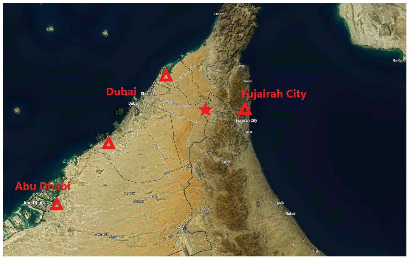
Figure 1A map (Buchhorn et al., 2020) showing the location of the measurement site with a red star. The red triangles represent the locations of significant oil refineries known by the writers. © Copernicus Service Information 2021.
The measurement campaign was conducted from February 2018 to February 2019. The in situ instruments were housed in a modified 20 ft (6.1 m) sea container. The container was next to a main farm building that was used as a weekend home, and there were only minor activities at the farm during the campaign. The temperature inside the container was kept stable, at around 25 ∘C, with two air conditioning units. A Doppler lidar (HALO Photonics) was situated on the top of the container in order to have as open a horizon for scanning as possible. A vertically pointing PollyXT lidar was placed next to the container. Both lidars were protected from the direct sunlight with sun shades.
2.2 In situ measurements
The air was sampled through a main inlet at height of 4.5 m above the ground, with a flow rate of 16.7 L min−1 and a cut-off nozzle of PM10. The air sample was dried with a Dekati diluter (dilution factor of 8.02). In this system, the dilution air is compressed, dried (dew point ), and filtered. After the dilution unit, which was located outside the container, the sample air was taken through a silica gel drying unit, which acted as a backup in case of compressor failure. This system kept the relative humidity well below 40 % as recommended (WMO/GAW Report 153; Baltensperger et al., 2003). The aerosol particle losses in this kind of dilution system have been reported before by Giechaskiel et al. (2009), who stated that the ejector diluter does not change the characteristics of the aerosol particle size distribution and that the aerosol particle losses are negligible.
The aerosol particle size distribution was measured with a differential mobility particle sizer (DMPS). The DMPS consists of a 28 cm long Hauke-type differential mobility analyser (DMA) (Winklmayr et al., 1991) with a closed-loop sheath flow arrangement (Jokinen and Mäkelä, 1997) and a condensation particle counter (CPC), TSI model 3772. The measured dry aerosol particle size range is from 7 to 800 nm, which is divided into 30 discrete bins. The DMPS data inversion was performed as described by Aalto et al. (2001) and Wiedensohler et al. (2012).
A cloud condensation nuclei counter (CCNc; Droplet Measurement Technology, Model CCN – 100; Roberts and Nenes, 2005) consists of a saturator unit and an optical particle counter (OPC). First, aerosol particles are brought to supersaturated conditions, and after that the number of activated droplets is counted with the OPC. The CCNc was operated at a flow rate of 0.5 L min−1 and in five different supersaturations (0.1, 0.2, 0.3, 0.6, 1.0). Each supersaturation measurement cycle was set to take 10 min, so one complete cycle took 1 h. The full cycle includes an additional supersaturation of 0.09 to allow the temperatures to drop and stabilise after measuring at a supersaturation of 1.0. The CCNc system also incorporated one extra feature that is not part of the standard CCNc system provided by the manufacturer; the additional feature enabled the CCNc to measure the fraction of activated aerosol particles as a function of size by size-selecting aerosol particles with a DMA (10–250 nm size range). To determine the fraction of activated aerosol particles at a certain size, the CCNc number concentration was compared to the number concentration of a CPC (TSI 3772 until end of October 2018, TSI 3310 during rest of the campaign) that was measuring in parallel with the CCNc. These scans were performed one supersaturation at a time from 10 to 250 nm (size ramp took 10 min) and then moving on to the next supersaturation to begin the next scan until all supersaturations were completed. The CCNc alternated between total CCN concentration and size-selected CCN concentration so that every second supersaturation sequence was with a size-selecting DMA in front so that each supersaturation cycle took 1 h to complete. The CCNc was calibrated for five different temperature gradients (corresponding to ΔT of 3–16 ∘C) using an aerosol generator (TOPAS, model ATM 226) with an ammonium sulfate solution (activation curve known) and a short Hauke-type DMA coupled with the CPC. The activation curve was calculated by measuring particles in a size range of 10–250 nm and comparing the particle counts between the CCNc and CPC. The activation curve for the different temperature gradients was used to calculate the supersaturations. After the supersaturations were calculated, a linear fit was used between the temperature gradients and calculated supersaturations, and the constants from the fit were given for the CCNc measurement programme as input parameters.
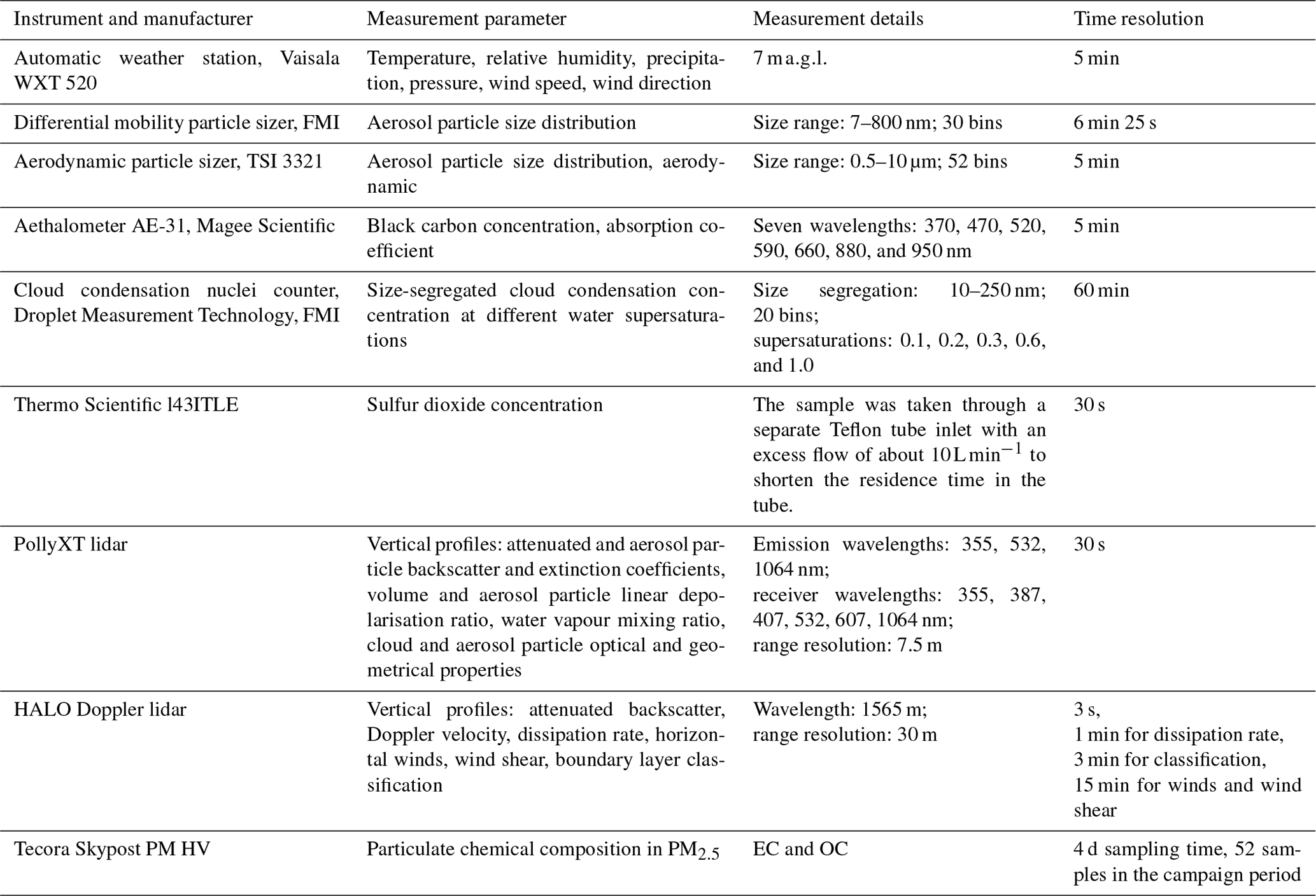
The SO2 concentrations were measured with a Thermo Scientific 43i-TLE using a 30 s time resolution. The sample air was taken through a separate Teflon tube inlet. The aerosol particle absorption coefficient was measured with an aethalometer (AE-31, Magee Scientific) at seven wavelengths (370, 470, 520, 590, 660, 880, and 950 nm) at 1 h time resolution. The list of instruments used in the measurement campaign is given in Table 1.
2.3 Offline sampling with filters
The PM2.5 samples were collected with an automatic outdoor station (Tecora Skypost PM HV) operating at a flow rate of 16.67 L min−1. The sampler automatically loaded a new filter every 96 h. There were 15 filters loaded in 1 cassette. The first filter was used as a blank filter and loaded and unloaded to the sampling position without any air flow. Aerosol particles were collected on pre-combusted 47 mm quartz fibre filters (Tissuquartz, PALL Life Science, Ann Arbor, USA). A total of 52 filters provided samples, with 6 filters providing blanks; the averaged concentrations from the blank filters were subtracted from the sample concentrations. The average blank concentrations of organic carbon (OC) and elemental carbon (EC) were 0.58 and 0.04 µg m−3, which were on average 19 % and 4 % of the sample concentrations, respectively. The average blank concentrations of analysed ions were below 0.02 µg m−3, which were on average below 5 % of the sample concentrations.
Punches of 1 cm2 were taken from the filters and analysed for OC and EC using thermal-optical techniques, which are based on the evolution of carbon species at different temperatures (Birch and Cary, 1996; Watson et al., 2005; Bauer et al., 2009). In the first phase, a sample is heated in steps from 550–900 ∘C using the EUSAAR-2 protocol (Cavalli et al., 2010) in an inert-helium atmosphere to remove OC. The organics may be pyrolysed to pyrolysed carbon (PC) during the inert phase, and this is observed by a decrease in the laser signal monitoring the transmittance through the sample matrix. In the second phase, oxygen is introduced, and the temperature is elevated stepwise as described by Cavalli et al. (2010). Carbon is oxidised to CO2, which is then converted to methane and detected by the flame ionisation detector. The PC formed during the temperature programme is compensated by determining the split point when the laser signal returns to its original value before pyrolysis. Methane was used as an internal standard and sucrose as an external standard.
Another filter punch (1 cm2) was used for analysing the main water-soluble inorganic ions (chloride, nitrate, sulfate, sodium, ammonium, potassium, magnesium, and calcium) using an ion chromatographic method based on the standard SFS-EN 16913:2017 (ambient air; standard method for measurement of , , Cl−, , Na+, K+, Mg2+, and Ca2+ in PM2.5 as deposited on filters). The filter sample was put in a test tube, extracted with 10 mL of ultrapure water for 30 min in an ultrasonic bath, and then directly filtered to the sampling vial using a syringe filter (Acrodisc 13, porosity 0.45 µm). Anions and cations were analysed using two identical ion chromatographs (Waters Corporation), which consisted of a separation module (Alliance 2695: an autosampler, an injector, and a pump) and a conductivity detector (Waters 432). In the anion ion chromatograph, calibration standards and samples were injected through the guard column (Waters Anion Guard-Pak) and analytical column (Waters IC-Pak A HR; 4.6×75 mm) using a borate–gluconate eluent and in the cation system through a guard column (Metrosep C4 Guard Metrohm) and analytical column (Waters IC-Pak C M/D; 3.9×150 mm) using an EDTA–HNO3 (ethylenediaminetetraacetic acid–nitric acid) eluent. The uncertainties in the analytical methods were 10 % or better for all analysed anions and cations.
2.4 Data processing
The data were first quality-checked and screened for outliers, such as extreme high or low concentrations, arising from an instrument malfunction or instrument maintenance. The aerosol particle data reported here are in standard temperature and pressure conditions (273.15 K, 1013.25 hPa).
The CCN data were processed in two parts. One part was the size-selected aerosol particles which were detected by both the CCN and a CPC concurrently to determine the sizes at which the aerosol particles could activate into cloud drops. The activation diameter where 50 % of the aerosol particles had been activated was determined by fitting the curve
to the ratio of CCN to CPC aerosol particle number concentration as a function of size. The curve fitting was done after manually checking the size distribution spectra, and, for a successful curve fit, the following criteria had to be met: (1) the activation curve should only cross the 0.5 (50 %) line once; (2) the curve should plateau out at higher diameters and remain roughly between 0.9 and 1.1.
The second part of the CCN data was the total number concentration of CCN at five different supersaturations. These data were aggregated into 10 min averages as that was the duration of the respective supersaturation measurement periods. This means that, for a particular supersaturation, the total CCN number concentration is represented by 10 min of data every second hour.
Aerosol particle water content and the conditions for cloud droplet activation can be predicted using the κ-Köhler theory (Petters and Kreidenweis, 2007). The value of κ describes an aerosol particle's hygroscopicity and hence the aerosol particle chemistry, with more hygroscopic aerosol particles having a higher κ value. When supersaturation increases, κ decreases because smaller aerosol particles are also activated to become CCN. The value of κ for the CCNc data was calculated at four different supersaturations (0.2, 0.3, 0.6, and 1.0) using
where Dc is the critical diameter, Sc is the supersaturation, σw is the surface tension of water, Mw is the molecular weight of water, R is the universal gas constant, T is the temperature, and ρw is the density of water. A typical range of κ for atmospheric aerosol particles extends from about 0.1 to 0.7, corresponding to nearly hydrophobic to very hygroscopic aerosol particle types (Petters and Kreidenweis, 2007).
The mass absorption cross-section (MAC) values used for black carbon concentration calculation were 39.53, 31.11, 28.13, 24.79, 22.16, 16.62, and 15.39 m2 g−1 (Arnott et al., 2005). The multiple-scattering enhancement correction factor (C0) value 3.5 was used based on World Meteorological Organization recommendations (GAW report no. 227; https://library.wmo.int/doc num.php?explnum id=3073, last access: 4 January 2022). The aethalometer measurement is known to suffer from filter loading and scattering artefacts. There are a number of different methods for correcting these artefacts, and here, the approach presented by Virkkula et al. (2007) was chosen.
The SO2 concentration data were first averaged hourly. After averaging, the data were corrected based on measured zero levels during the campaign (Komppula et al., 2017).
All the results are presented in local time (UTC+4 h).
2.5 Halo Doppler lidar measurements
The Halo Photonics Streamline Doppler lidar is a pulsed lidar operating at 1565 nm using heterodyne detection (Pearson et al., 2009). The instrument has full hemispheric scanning capability and provides range-resolved profiles of the backscattered signal intensity, in terms of signal-to-noise ratio (SNR), and radial Doppler velocity. For this campaign, the instrument was operated with a radial resolution of 30 m, covering a range from 90 to 9600 m. Additional instrument technical specifications and configurations are given in Table A1. The scan schedule selected for the campaign comprised vertical stare mode with 3 s integration time interspersed with a set of velocity-azimuth-display (VAD) scans every 15 min at three different elevations from horizontal: 15, 45, and 70∘. Each VAD scan contained 24 rays equally spaced in azimuth with an integration time of 2 s per ray, except for the highest elevation scan, at 70∘, which had an integration time of 3 s per ray.
Background correction of SNR was performed as described in Manninen et al. (2016) and Vakkari et al. (2019) in order to obtain reliable uncertainty estimates for SNR and radial Doppler velocity (Rye and Hardesty, 1993). Profiles of calibrated attenuated backscatter coefficient were then derived from the vertical profiles of corrected SNR using the telescope function determined with the method of Pentikäinen et al. (2020) and the dissipation rate of turbulent kinetic energy calculated from the variability in the vertical Doppler velocities (O'Connor et al., 2010).
The vertical profile of horizontal wind was calculated from the VAD scans (Päschke et al., 2015), with the lower-elevation scans providing better vertical resolution closer to the surface. The horizontal wind calculation assumes homogeneity, which may not be valid under strongly turbulent conditions, and the lower-elevation scans also suffer less from possible violation of this homogeneity assumption.
The presence of turbulent mixing is diagnosed from the dissipation rate (O'Connor et al., 2010), and the combination of attenuated backscatter coefficient, vertical velocity skewness, dissipation rate, horizontal wind, and vector wind shear is used to derive a boundary layer classification (Manninen et al., 2018). This boundary layer classification identifies the mixing layer height and also identifies which regions of mixing are connected to the surface. During the daytime, mixing connected to the surface is assumed to be convective (buoyancy production), but there are also cases where there is mixing at night connected to the surface arising from wind shear. For our purposes we assigned daytime mixing associated with convection to periods of mixing observed between 05:00 and 20:00 LT and nighttime mixing to periods of mixing observed between 20:00 and 05:00 LT.
3.1 Meteorological observations
The meteorological observations were averaged hourly, with a 1 h data coverage of 94 %. The highest hourly mean temperature of 48 ∘C was measured in July 2018, and the lowest hourly temperature of 10 ∘C was measured in February 2019. The hourly averaged maximum wind speed measured at the station was 17.5 m s−1 in May 2018. The minimum relative humidity of 6 % was measured in March 2018 and the maximum, 90 %, in November 2018. The measured ambient pressure was stable during the measurement period (minimum 972.6 hPa, maximum 1004.2 hPa). Rain rarely reached the surface, usually evaporating as it fell into dry layers below the cloud level – a frequent characteristic for rainfall events in this region (Wehbe et al., 2019, 2020); only eight rain events were observed at ground level during the campaign. The events were very short, lasting less than 1 h each.
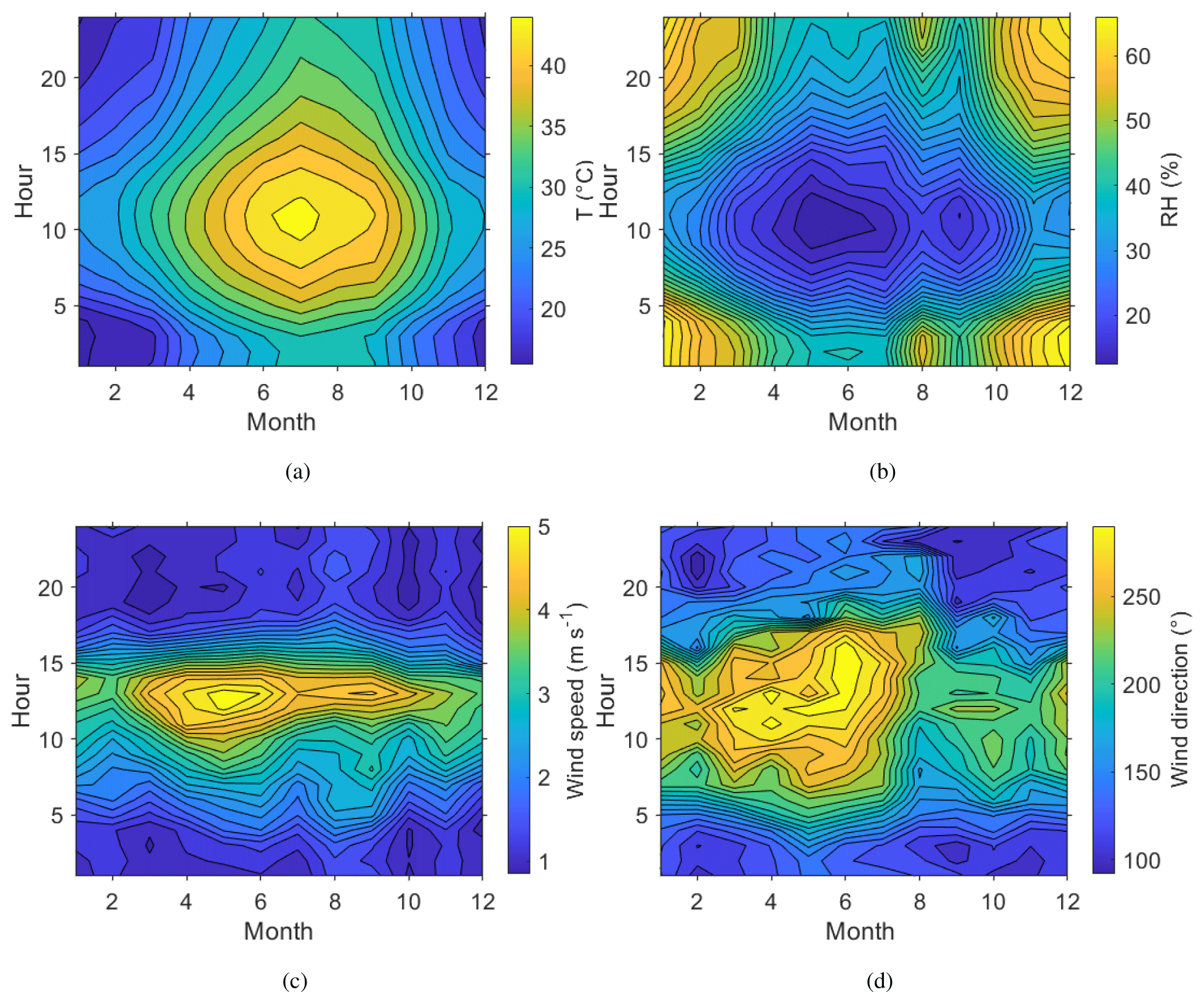
Figure 2Seasonal and diurnal variation in surface (a) temperature, T (∘C); (b) relative humidity, RH (%); (c) wind speed, WS (m s−1); and (d) wind direction, WD (∘). All measurements made at 7
Daily and annual variation in meteorological conditions during the campaign year are shown in Fig. 2. The highest temperatures were measured at noon during the summer months, when the relative humidity also reached its minimum. The highest wind speeds were measured in early summer. The daily variation in the wind direction at the site was very distinctive, following a similar pattern every day, turning from the eastern direction (Gulf of Oman) to the north-west (Arabian Gulf) during the day and then back to the east after the sun had set. From March to August the variation between these two directions was more pronounced than from September to February. The wind speeds at the surface were in general quite low, averaging only 2.2 m s−1. The wind speed showed a clear daily pattern, with the nights typically very calm and stronger winds during daytime, peaking around noon.

3.2 Aerosol particle properties
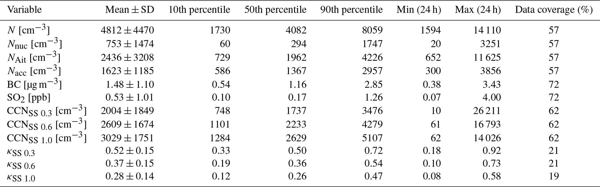
Chemical and physical properties of aerosol particles were investigated by statistical means. The statistics for daily means of different measured aerosol particle properties are shown in Table 2. The mean aerosol particle total number concentration was 4812 cm−3, which was much lower than the mean total concentration of 10 630 cm−3 measured by Lihavainen et al. (2016) in Saudi Arabia. We also compare our measurements to those made in another arid region in South Africa. Vakkari et al. (2013) observed median concentrations of 1856 and 7805 cm−3 in the size range of 12–840 nm at Botsalano and Marikana in South Africa, and Laakso et al. (2012) observed a mean aerosol particle total number concentration of 6310 cm−3 in the size range of 10–840 nm in the polluted Highveld area in South Africa, where several coal-fired power plants were located around the measurement site. The mean SO2 concentration of 0.53 ppb is equivalent to 1.4 µg m−3, which was consistent with the mean SO2 concentrations of 2.6–4.2 µg m−3 measured by Al Katheeri et al. (2012) in Al Mirfa, United Arab Emirates (UAE), during 2007–2009. The mean black carbon concentration measured during this campaign was lower than the mean concentration of 2.1 µg m−3 observed in Saudi Arabia by Lihavainen et al. (2016). The observed CCN number concentration was highest when measuring at a supersaturation of 1.0, with the largest κ parameter at a supersaturation of 0.3.
Table 2Mean; standard deviation; 10th, 50th, and 90th percentile; minimum and maximum values of daily means; and data coverage for different measured variables. The size ranges for different aerosol particle modes are 10–25 nm for nucleation mode aerosol particles, 25–100 nm for Aitken mode aerosol particles, and 100–800 nm for accumulation mode aerosol particles. N is total number concentration of all particles measured with the DMPS. Nnuc is the total number concentration of nucleation mode aerosol particles. NAit is the total number concentration of Aitken mode aerosol particles. Nacc is the total number concentration of accumulation mode aerosol particles. BC is black carbon. CCNSS 0.3 is the total number concentration of cloud condensation nuclei in supersaturation 0.3, CCNSS 0.6 in supersaturation 0.6, and CCNSS 1.0 in supersaturation 1.0; κSS 0.3 is κ value in supersaturation 0.3, κSS 0.6 in supersaturation 0.6, and κSS 1.0 in supersaturation 1.0.
3.2.1 Aerosol particle chemical components
Chemical analysis indicated that sulfate had the highest contribution (around 50 % of the analysed mass) to aerosol particle composition in the UAE (Table 3, Fig. 3), and it was mainly in a form of ammonium sulfate ((NH4)2SO4). The contribution of sea salt to was small (up to 4 %) at the site, indicating that the majority of the sulfate was of anthropogenic origin. Sulfate and SO2 concentrations were correlated with each other, having higher concentrations in spring and summer. The annual average sulfate mass concentration in the UAE was high (10.34 µg m−3; Table 3, Fig. 3). There are two oil refineries located on the eastern and western side of the measurement site: Fujairah oil refinery around 40 km in the east and Sharjah oil refinery around 70 km in the west (Fig. 1). The refineries are assumed to be the main reason for the measured high sulfate mass concentration at the site. When compared to other studies, the annual average sulfate mass concentration in the UAE was over twice as high as concentrations measured in rural South Africa sites and 5 times higher than concentrations measured in an urban area in the USA (Aurela et al., 2016; Chan et al., 2018). On the other hand, Wu and Wang (2007) measured 1.5 times higher 24 h filter sulfate mass concentration in a suburban area 45 km north-west of the centre of Shanghai and over 2 times higher concentration measured in a mountainous area 50 km north of the centre of Beijing. The carbonaceous components (OC and EC) made the second-highest contribution to aerosol particle mass (Table 3). EC forms during incomplete burning, and its origin is always primary, whereas OC can be primary or secondary. A rough guide to the origin of the carbonaceous aerosol particles is given by the ratio between OC and EC concentrations if only one major EC source (traffic or biomass combustion) is dominant (Turpin and Huntzicker, 1995). The OC-to-EC ratio was 2.81, which resembles values measured at urban background areas (e.g. Aurela et al., 2011). EC and BC showed a strong correlation, and, on average, the BC-to-EC ratio was 2.2. We also observed calcium, magnesium, sodium, and chloride (Table 3, Fig. 3), which are typically observed in the coarse-aerosol particle size fraction (>2.5 µm). These ions mostly originate from soil and sea salt. The ratio of cations to anions was close to 1, so the ion balance was neutral. Potassium showed higher concentrations during May 2018 (Fig. 3), which may be a result of biomass burning. However, a similar increase was not seen for BC.
Table 3PM2.5 concentrations and statistics for EC, OC, and their ratio and water-soluble ions, measured in 52 4 d samples. Units for components are µg m−3.
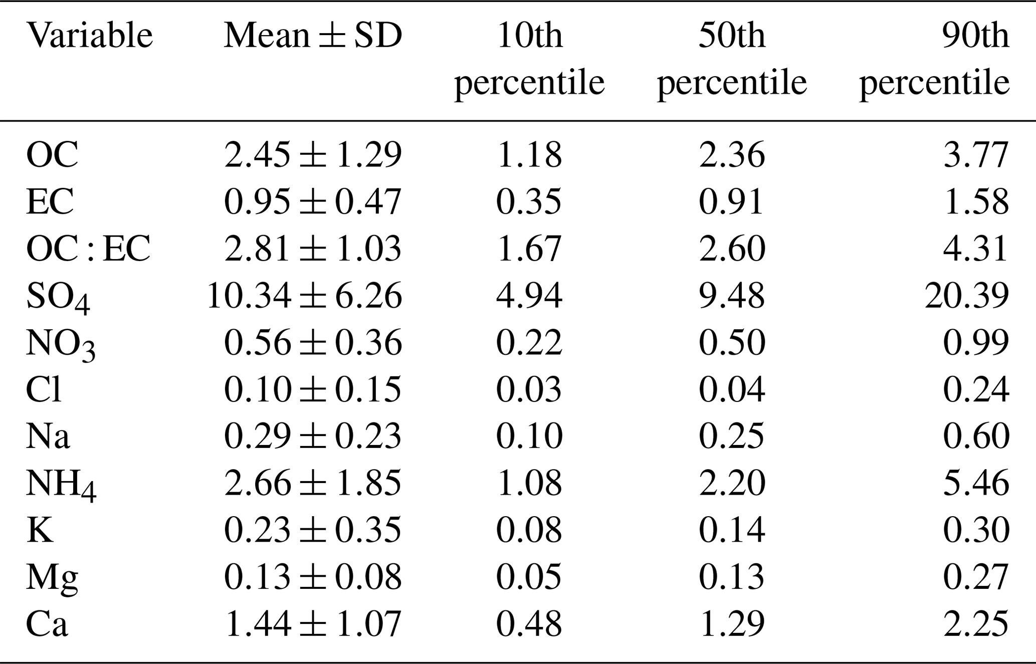
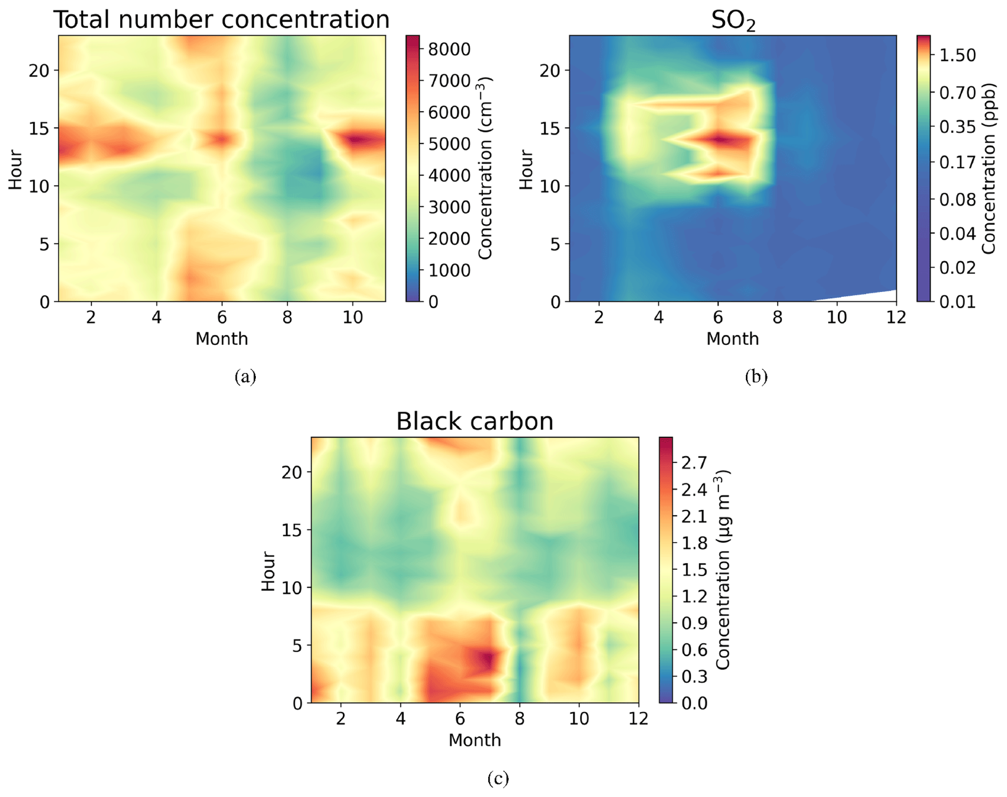
Figure 4Seasonally diurnal contour plots of (a) aerosol particle total number concentration (cm−3) measured with the DMPS, (b) SO2 concentration (ppb) measured with the SO2 gas analyser, and (c) black carbon mass concentration (µg m−3) measured with the aethalometer. Hourly median values have been used.
3.2.2 Daily and intra-annual variation
Figure 4a shows that the total aerosol particle number concentration usually peaked after local noon. This diurnal maximum is dominated by frequently observed secondary new-particle-formation (NPF) events that had a clear diurnal cycle, together with a potential change in aerosol particle population due to the change in wind direction during the day. The total aerosol particle number concentration was lowest during late summer and early autumn and relatively constant during the rest of the year. Figure 5 shows aerosol particle total number concentration separated into nucleation, Aitken, and accumulation modes. Nucleation mode aerosol particles have the highest concentration at noon, whereas accumulation mode aerosol particles have their highest concentrations during night. This is an expected result because accumulation mode aerosol particles are aged aerosol particles that have the longest lifetime in the atmosphere and are trapped in the nighttime stable layer, whereas nucleation mode aerosol particles are newly formed and grow fast to larger sizes during the day. This diurnal cycle is typical for locations experiencing NPF events and was also observed by Lihavainen et al. (2016) in western Saudi Arabia. The growth of the boundary layer also impacts the diurnal cycle of the concentration in accumulation mode aerosol particles through the dilution of the aerosol particles into a larger volume as the boundary layer depth increases.
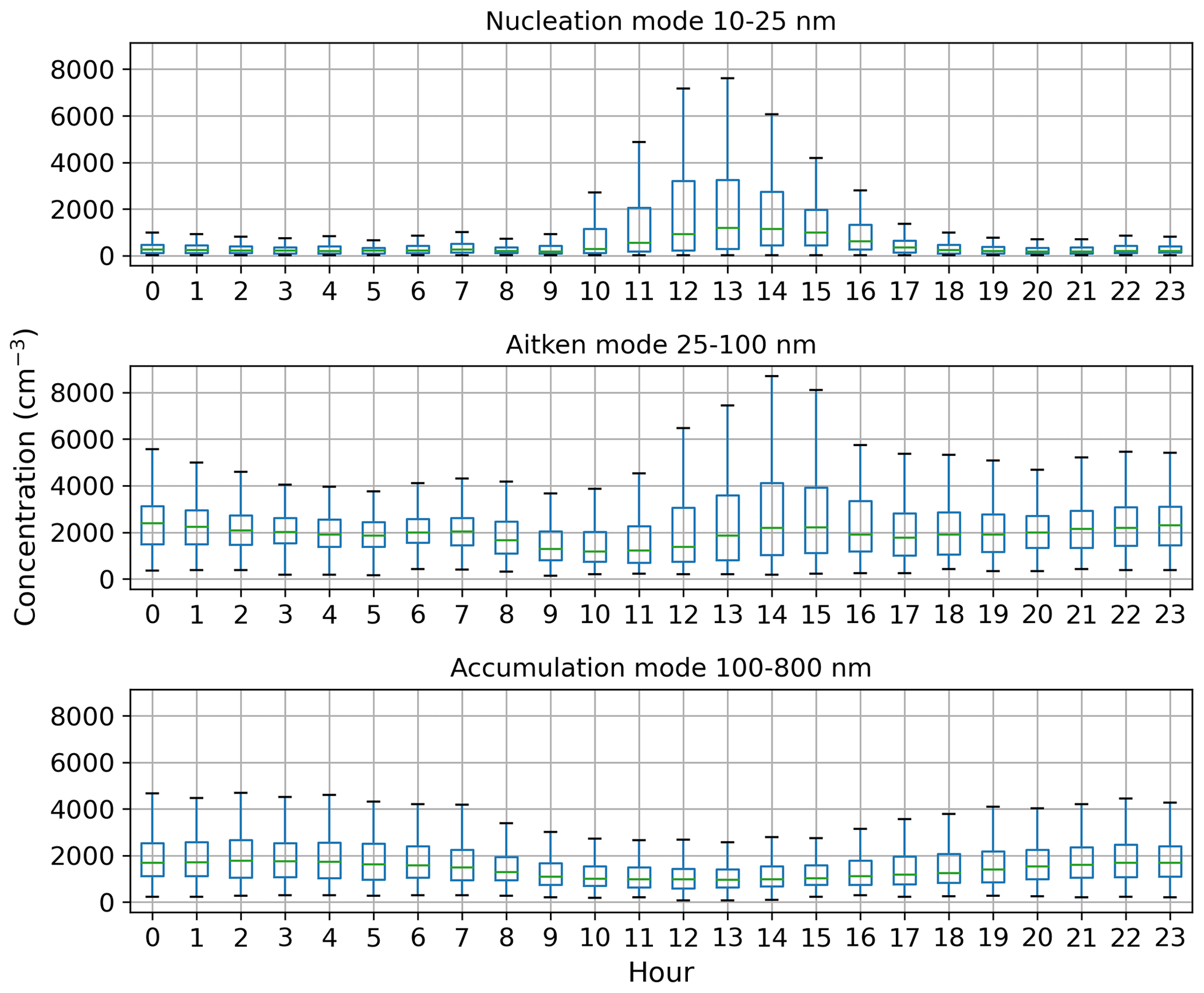
Figure 5Box-and-whisker plots for hourly median concentration values (cm−3) of different aerosol particle modes. The central line (green) in each box indicates the median, and the bottom and top lines of the boxes indicate the 25th and 75th percentiles. The whiskers mark the most extreme data points that are not considered to be outliers (within a range of 1.5× interquartile range from the edges of the box).

Figure 6Seasonally diurnal contour plots of (a) κ parameter, (b) CCN number concentration (cm−3), and (c) activation fraction (CCN/CN) in different supersaturations. Hourly median values have been used.
Similar to aerosol particle number, very strong diurnal and annual cycles were observed in SO2 concentrations (Fig. 4b). The highest SO2 concentrations were observed around midday, especially during spring (March to June). The wind direction at midday was coming from west or north-west (Fig. 2d), where sources of SO2 exist, such as Dubai. Lower concentrations at other times of the year are most likely because of the change in the prevailing midday wind direction to directions where no strong or nearby sources exist. The black carbon concentration was highest during the night (Fig. 4c), with low concentrations during the day presumably due to the increase in mixing volume in the boundary layer and increased wind speed. Black carbon concentration did not show any clear seasonal dependence.
The daily and annual variation in κ parameter at supersaturations of 0.3 and 1.0 is shown in Fig. 6a. The κ parameter decreased with supersaturation (SS); at SS0.3, κ varied from 0.17–1.16 and at SS1.0 from 0.01–0.87, with the highest values at a supersaturation of 0.3. The fraction where 50 % of aerosol particles activate into cloud droplets is called the activation diameter (D50) and is used when calculating κ. D50 was 68±6 nm at SS0.3 and 39±7 nm at SS1.0. This result suggests that aerosol particles at the critical diameter at SS0.3 had different chemistry and were more hygroscopic than other aerosol particles in the region (Sarangi et al., 2019), which means that smaller aerosol particles were less hygroscopic. The κ parameter had higher values during daytime, which suggests that there are more sulfate aerosol particles present from the NPF events, that the wind direction means there is significant transport of hygroscopic aerosol particles to the site, that sulfuric acid originating from SO2 condensates on pre-existing aerosol particles, or that all are affecting concurrently. During nighttime there are more BC aerosol particles present (Fig. 4c), which are less hygroscopic; κ showed a small decrease in early autumn, and there was a small decrease also in early spring.
The activation diameter of aerosol particles decreases when supersaturation increases, which can be seen in Fig. 6b, showing higher CCN concentrations during nighttime, when there were more long-lived and larger accumulation mode aerosol particles and black carbon present (see Figs. 5 and 4c). The CCN number concentrations were highest in early summer. The CCN number concentration decreased significantly in early autumn. This may be due to a change in the environmental circumstances, i.e. a change in the prevailing midday wind direction transporting aerosol particles from different sources.
The activation fraction (CCN CN) describes the number of aerosol particles that are activated to CCN. Figure 6c shows the diurnal and monthly changes in activation fraction; the highest activation fractions were measured in the morning and evening, when the CCN number concentration was also highest; κ values are highest during daytime, and when we consider the diurnal variation in different aerosol particle sizes shown in Fig. 5, it seems that size is more important for CCN activation than chemistry at this location. The activation fraction is smaller during the daytime because there are more small non-CCN active aerosol particles present. The reason for high daytime κ values may be due to the presence of hygroscopic aerosol particles such as sea salt or sulfate from anthropogenic sources that have been transported to the site by westerly winds. There was a peak in the activation fraction in early spring, after which the activation fraction smoothly decreased towards the end of the year. Activation fraction was the lowest in the beginning of the year.
The aerosol particle properties followed similar daily cycle. During late morning the wind direction typically changed from the eastern direction to the north-west. Before and during the change we observed lower aerosol particle total number concentrations compared to midday and also lower SO2 concentrations. On the other hand, the BC concentration was higher before the change in wind direction, after which the wind speed started to increase. The κ parameter was lower, but CCN number concentration and activation fraction were higher. During the afternoon, when the wind was coming from the north-west, we observed a peak in aerosol particle total number concentration and in SO2 concentration, whereas the BC concentration decreased, presumably due to dilution in the deeper boundary layer. The κ parameter was higher during the day, but the CCN number concentration and activation fraction decreased. After sunset and during the night, the wind direction changed back to the eastern direction, with the aerosol particle total number concentration and SO2 concentration decreasing and the relative portion of accumulation mode aerosol particles increasing, BC concentration starting to increase, κ parameter decreasing, and CCN number concentration and activation fraction starting to increase.
3.3 Impact of the boundary layer on aerosol particle properties
3.3.1 Turbulent and non-turbulent boundary layers
Aerosol particle properties at our UAE measurement site showed a clear diurnal cycle. This corresponds to the strong diurnal cycle in boundary layer evolution and the wind direction observed in the Doppler lidar profiles. To investigate the impact of the boundary layer evolution and wind direction on aerosol particle properties, we separated our analysis into three classes of boundary layer conditions using the boundary layer classification derived from Doppler lidar: daytime mixing (convective boundary layer), nighttime where mixing was present, and nighttime with no mixing present (calm). We assume that vertical mixing will dilute the concentrations from ground-level sources. When there is no mixing during the night we expect an increase in concentrations as the emissions from local sources are trapped in the surface layer with only advection providing transport at ground level and limited dilution in the vertical dimension. One source of turbulent mixing in the boundary layer at night is low-level wind jets with significant shear (Marke et al., 2018).
The median value of the SO2 concentration from each boundary layer class varied from 0.13–0.2 ppb, with the highest values during daytime mixing (Fig. A1a). This is attributed to the transport of pollution from Dubai and other urban areas (see prevailing wind direction during the day; Fig. 2d). At night, concentrations were higher when there was no mixing because of the limited dilution in the vertical. The median black carbon concentration at the surface varied between 0.9–1.9 µg m−3 in different boundary layer circumstances (Fig. A1b) and was more directly connected to the presence of boundary layer mixing, being lower during the day and higher during nights with no mixing.
Figure 7a shows κ values calculated for the three different boundary layer conditions. Median κ values ranged from 0.4–0.6, with the highest median value and largest variability during daytime mixing. This indicates that larger and more hygroscopic aerosol particles are present during the day, whether emitted locally or transported to the measurement site. One potential source is the elevated daytime SO2 concentrations from which sulfate aerosol particles can form. A smaller κ during nighttime is typical for anthropogenic aerosol particles (Hung et al., 2014; Cheung et al., 2020).

Figure 7Box-and-whisker plots of hourly median values for three boundary layer conditions for (a) κ parameter, (b) CCN number concentration (cm−3), and (c) activation fraction (CCN/CN) at a supersaturation of 0.3. The central line in each box indicates the median, and the bottom and top lines of the boxes indicate the 25th and 75th percentiles. The whiskers mark the most extreme data points that are not considered to be outliers.
Figure 7b shows that the median CCN number concentration was close to 1500 cm−3 when there was turbulent mixing present, whether during the day or at night, and was about 2000 cm−3 during calm nights. The lowest concentration values, observed during the day, are when there are more nucleation mode aerosol particles present, and there are more large accumulation mode aerosol particles present at night (Fig. 5).
Figure 7c shows activation fraction for the three different boundary layer conditions. Taken annually, an average of 40 %–50 % of aerosol particles were able to activate as CCN at SS = 0.3, with the highest median activation fraction being observed during turbulent conditions at night. This is probably due to the higher relative contribution of larger accumulation mode aerosol particles, which are more easily activated to CCN. The reason why the activation fraction is higher during turbulent rather than calm nights is probably due to the entrainment of the residual layer above back into the nocturnal boundary layer. The aerosol particle properties of the residual layer, which is formed from the decaying deep daytime boundary layer above the nocturnal boundary layer after sunset, evolve slowly from the aerosol particle properties of the daytime convective boundary layer. The residual layer is rich with larger aerosol particles, which, if mixed down into the nocturnal boundary layer, would increase the number of CCN-activated aerosol particles observed at the surface during nighttime. Another possibility is that a calm nocturnal layer leads to a build-up of small (non-CCN active) aerosol particles, which would be more effectively scavenged in a turbulent layer. Low activation fractions during daytime are probably due to NPF events occurring during the day, generating large numbers of small and hence less easily activated aerosol particles.
SO2 concentrations had their highest values during daytime mixing. More pronounced differences were seen in black carbon concentrations under different boundary layer conditions; higher concentrations were observed during calm nights, indicating that the source of black carbon is likely to be local and disperses in turbulent conditions. The highest median κ values were observed during daytime mixing, indicating that larger and more hygroscopic aerosol particles are present in the boundary layer during daytime. We observed the lowest CCN number concentrations during daytime, when there are more newly formed nucleation mode particles present. The highest activation fractions were observed during nighttime, when the boundary layer was turbulent, attributed to the entrainment of particles in the residual layer above down into the boundary layer. These results show that different boundary layer conditions affect aerosol particle properties at the site.
3.3.2 Boundary layer height
We also studied the impact of daytime boundary layer height on the aerosol particle measurements made at the surface. We took all daytime measurements for each day and binned these into four height ranges using the maximum boundary layer height for that day. Each bin was about 250 m wide to give approximate bin top heights at 1.5, 1.75, 2, and 2.25 km (1245–1515, 1515–1755, 1755–1995, and 1995–2265 m).
The median SO2 concentration showed a dependence on maximum boundary layer height (Fig. 8a), with median values increasing with maximum boundary layer height from 0.2–0.25 ppb up to boundary layer heights of 1.75–2 km; the highest median value and the greatest range in values were for boundary layer heights of 1.75–2 km. However, black carbon concentration (Fig. 8b) showed a slight decrease with increasing maximum boundary layer height. Median concentrations varied between 1.0–1.1 µg m−3, with the lowest median concentration measured in the same height range as the maximum median SO2 concentration. These results suggest that BC concentrations are dominated by local sources, whereas SO2 sources are not. The residual layer is one source of SO2, which requires the boundary layer to grow and entrain this source into the boundary layer. The other source is transport within the boundary layer, evidenced by the strong SO2 concentration dependence on wind direction.

Figure 8Box-and-whisker plots of hourly median values for a range of boundary layer heights for (a) SO2 (ppb), (b) black carbon (µg m−3), and (c) activation fraction (CCN/CN) at a supersaturation of 0.3. The central line in the boxes indicates the median, and the bottom and top lines of the boxes indicate the 25th and 75th percentiles. The whiskers mark the most extreme data points that are not considered outliers. The boundary layer height value refers to the top of each height bin.
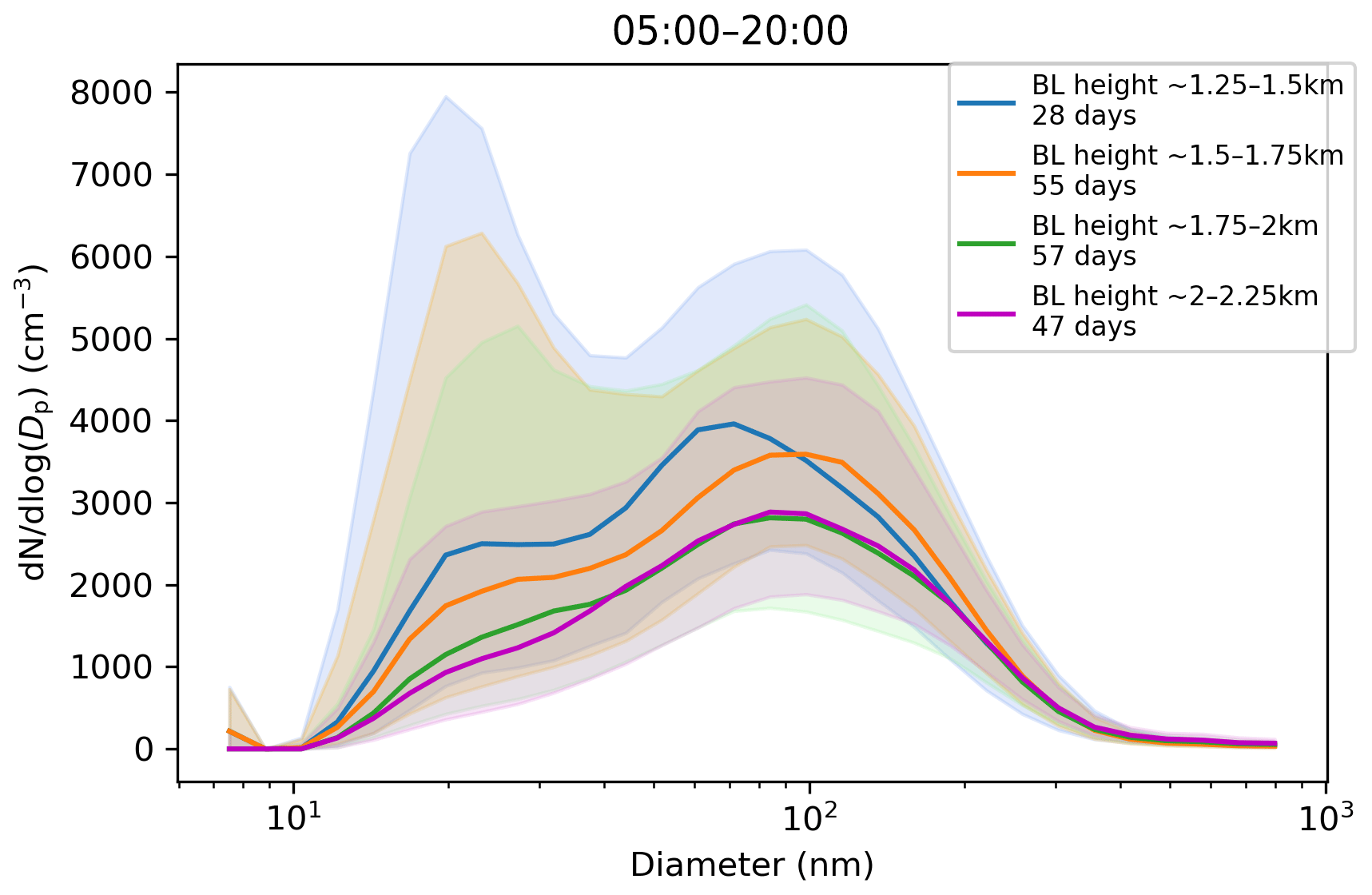
Figure 9Impact of boundary layer height on the aerosol particle size distribution in (cm−3) measured at the surface during daytime mixing (from 05:00 to 20:00 LT). Hourly median values are used. Number of days included in each boundary layer height range is given in the figure legend. The shaded areas indicate the median ± the interquartile range of the distributions.
Median CCN concentrations and κ values (not shown) displayed little dependence on maximum boundary layer height, but the median CCN-activation fraction, which ranged from 40 %–45 %, did increase with maximum boundary layer height (Fig. 8c). Figure 9 shows that the aerosol particle size distribution did change with maximum boundary layer height, with number concentrations reducing as the boundary layer height increased. The growing boundary layer dilutes the aerosol particles from local sources into a larger volume, but at the same time, there is entrainment of aged aerosol particles in the residual layer back into the boundary layer. The change in the shape of the size distribution explains the change in CCN-activation fraction, so although there is no change in the CCN concentration itself, the reduction in the number of small aerosol particle sizes, which are less likely to activate, with increasing maximum boundary layer height will increase the CCN-activation fraction with increasing maximum boundary layer height.
3.3.3 New-particle-formation events
We defined NPF event days based on the number concentration in the 16.8 nm size bin, with a threshold value of 3000 cm−3 () being exceeded in order to be classified as an event day. The relative proportion of event days was very high, with 178 event days from a total of 224 measurement days. The starting time of NPF events was defined using the concentrations in the 10.4 nm size bin. We identify that an event has started when the concentration in this size bin increases by at least 300 particles cm−3 (). The actual event starting time is then estimated based on the growth rate estimated visually from six DMPS size concentration figures (Fig. B1) where there was a very clear NPF event. Our estimate for the mean growth rate was (1 standard deviation), which is consistent with the median growth rate of 7.4 nm h−1 observed by Hakala et al. (2019) in Saudi Arabia. The visually estimated growth rates ranged between 2.5 and 10 nm h−1. We subtracted 2 h from the identification time obtained from analysing concentrations in the 10.4 nm size bin to derive the time when these aerosol particles were about 1 nm in size based on the estimated growth rate. We should highlight here that the growth rate as defined from the DMPS measurements is not directly applicable for the smallest particles, which usually have much lower growth rates (Kulmala et al., 2004). We assume that the growth rate for clusters 1.5–3 nm in diameter is about a quarter of the growth rate at 10.4 nm (Kulmala et al., 2004), which is 1.7 nm h−1. Thus, we assume that it takes about 1.5–2.5 h for clusters of particles 1 nm in size to grow to 10.4 nm and use this reasoning to justify the 2 h delay between the probable NPF event starting time and the event being observed with our measurement instrumentation. The start hours for NPF events determined in this manner are presented in Fig. 10a. NPF events usually started around 07:00–09:00 LT. This was compared with the time that the boundary layer started to grow (Fig. 10b). We defined the boundary layer growth start time based on the value of the dissipation rate of turbulent kinetic energy derived from Doppler lidar, ϵ, exceeding at a height of 225 m. Boundary layer growth at this height usually started around 09:00–10:00 LT, and if we consider that it started a little earlier at the surface, it is quite consistent with the estimated NPF event typical starting time.
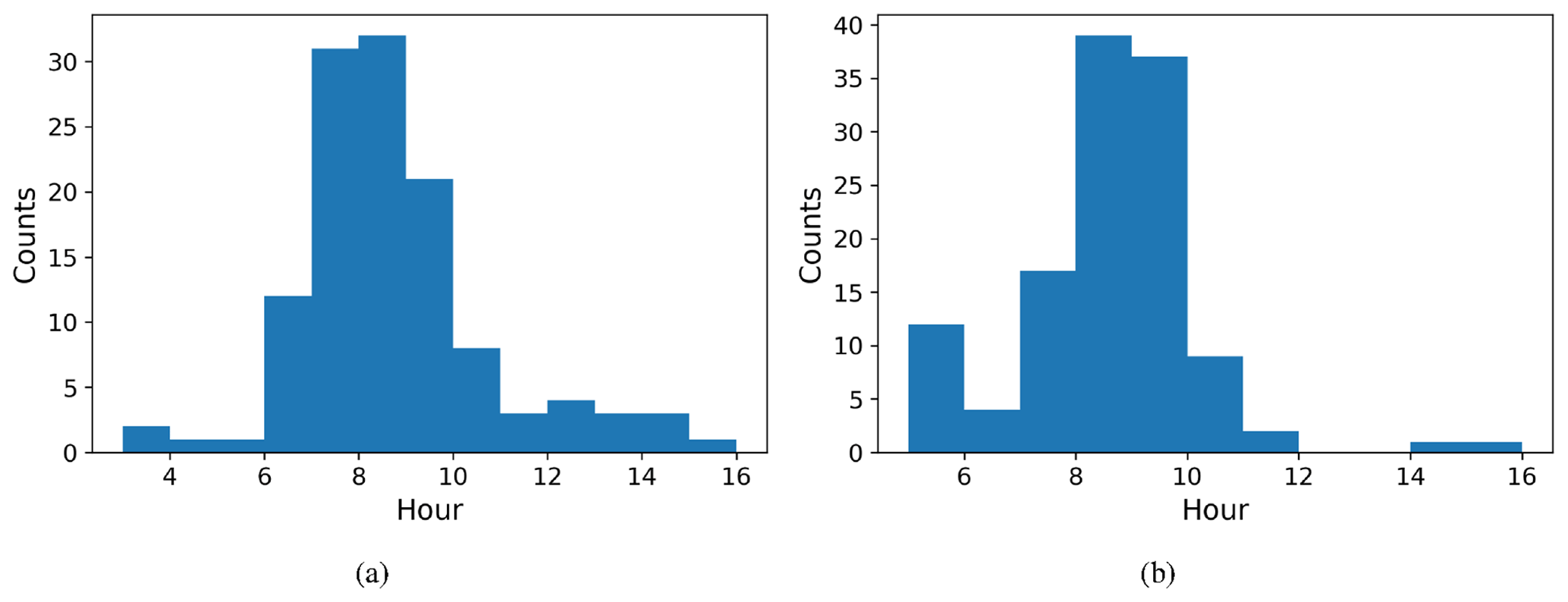
Figure 10Histograms of start time for (a) NPF events and (b) boundary layer growth. The time axis is local time (hours UTC+4).
Our explanation for the correlation between the starting time of boundary layer growth and the start of NPF events is that precursor gases from elevated levels are mixed down to the surface and initiate an NPF event at the surface or that the NPF event is initiated aloft, which has been observed by several studies (Größ et al., 2018; Lampilahti et al., 2021; Brus et al., 2021), and the newly formed particles are then measured at the surface once they are entrained within the growing boundary layer.
3.4 Case studies
The evolution of the boundary layer was very similar day to day at this location in the UAE, with a significant residual layer also present on most days. Here we show three representative case studies to examine how the evolution of the boundary layer impacted aerosol particle properties measured at the surface: a deep boundary layer with horizontal transport aloft, a shallow boundary layer, and a deep boundary layer with a stagnant residual layer and no significant horizontal transport aloft. Except for the horizontal transport loft, the dynamical evolution of the two deep boundary layers appeared to be very similar, with both growing boundary layers entraining residual layers containing significant numbers of aerosol particles. We chose to focus on conditions between midnight and 11:00 LT to concentrate on the time period which was most similar day to day and to avoid including daily dust events and other large-scale dynamical mechanisms such as sea breezes.
3.4.1 Deep boundary layer with horizontal transport aloft
We selected 19 May 2018 as a representative deep-boundary-layer case study. The boundary layer height reached a maximum of 2775 m on this day. Figure 11a shows that the surface was calm at night, and the convective boundary layer mixing started at the surface around 07:00 LT. SO2 concentrations (Fig. 11b) remained low at night and then rose rapidly as the convective boundary layer grew. There was a strong peak in aerosol particle number concentration before the mixing started (Fig. 11c), and then the sign of an NPF event was seen at 09:00 LT. The start time for the NPF event was therefore assumed to be 2 h earlier, at 07:00 LT, which was when the convective boundary layer mixing started, and the SO2 concentration began to increase. During the night, wind speeds were light at the surface (<5 m s−1) and from the south, but there was a stronger wind jet above at around 1 km height (Fig. 11d), which was coming from the north-north-west (Fig. 11e), i.e. from Dubai and other conurbations. Moderate turbulence arising from the wind shear associated with this wind jet can also be observed. The wind direction at the surface changed towards the north-west at 07:00 LT, which also coincides with when SO2 concentrations increased, although the surface winds remained light.
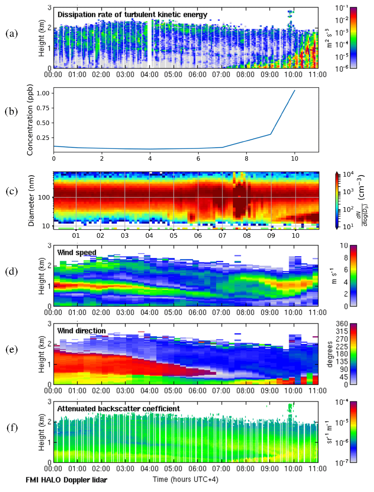
Figure 11Deep-boundary-layer case with transport aloft on 19 May 2018. (a) Time–height plot of dissipation rate of turbulent kinetic energy, ϵ; (b) SO2 concentration (ppb) measured at the surface; (c) aerosol particle size distribution measured at the surface (the colour indicates the concentration in cm−3); and time–height plots of (d) wind speed, (e) wind direction, and (f) attenuated backscatter coefficient. For all panels, the time axis is local time (hours UTC+4). The measurements in panels (a, d, e, and f) were obtained from the HALO Doppler lidar.
Occasional strong peaks in DMPS concentrations can be seen between 05:00 and 08:00 LT. At this time the boundary layer height had not yet grown significantly, so these are most likely arising from local sources, and this increase is also seen in the Doppler lidar attenuated backscatter coefficient (Fig. 11f) close to the surface. Such peaks are not seen later in the day once the boundary layer has grown deeper, and hence we suspect that any local pollution source is rapidly dispersed in a deeper boundary layer. Figure 11f also shows that there are considerable aerosol particles present in the residual layer which are then entrained into the boundary layer as it grows; hence the aerosol particle number concentration at the surface remains high.
3.4.2 Shallow boundary layer
The shallow-boundary-layer case study (21 February 2018) had a maximum boundary layer height of 1215 m. As in the deep-boundary-layer case study the surface was mostly calm at night, with Fig. C1a in the Appendix showing the convective boundary layer mixing starting around 09:00 LT. This coincides with an increase in SO2 concentrations and a change in the wind direction to the north-west. A peak in number concentration of smaller aerosol particles at 10:00 LT indicates an NPF event starting at around 08:00 LT. However, SO2 concentrations were also elevated during the night, when surface winds were also from the north-west, and then reduced by 04:00 LT as the wind direction changed to the west and south-west. The wind direction had changed at the surface by 02:00 LT, but some turbulent mixing was also present from 02:00–03:00 LT, which may also have helped continue to mix some elevated SO2 to the surface until the wind direction aloft had also changed.
Figure C1f shows again that there are considerable aerosol particles present in the residual layer which are then entrained into the boundary layer as it grows; hence the aerosol particle number concentration at the surface remains high.
3.4.3 Deep boundary layer, stagnant residual layer aloft
The case study for 8 May 2018 presents a case similar to the deep-boundary-layer case except that the weak winds aloft mean that the deeper residual layer above has not moved very far horizontally since the previous day and is hence stagnant. In addition, the residual layers have different aerosol particle properties to the surface layer formed overnight. As in previous cases, the surface was calm, and convective boundary layer mixing commenced around 08:00 LT (Fig. D1a). Surface SO2 concentrations were low throughout most of the night, and the wind direction at the surface remained east or south. Surface SO2 concentrations rapidly increased once convective mixing started, even though the wind direction at the surface was from the south. However, there was an elevated layer aloft advecting from the north-west to the north, which the boundary layer rapidly grew into after 08:00 LT, and we attribute the increase in SO2 concentration to the entrainment of this layer. This can also be seen in Fig. D1f, with the elevated layer no longer visible after 10:00 LT. Small aerosol particles were present at the surface during the night but disappeared once the convective mixing started, and SO2 concentrations also began to decrease again after this layer had been entrained. Winds in the deeper residual layer above this were low, so once the source had been depleted, there was no advection bringing more SO2.
3.4.4 Aerosol particle size distribution
For the three case study days selected, Fig. 12 showed the change in aerosol particle size distribution before and after convective mixing started at the surface. There is little change in concentration in the larger sizes (diameters >50 nm) for both the deep- and shallow-boundary-layer cases selected, but there is significant increase in the concentrations of smaller aerosol particles (diameters <30 nm). We attribute the change in small aerosol particle number concentration to NPF, which starts at a similar time to the daytime convective mixing. Note that the small mode peak is at smaller sizes for the shallow-boundary-layer case, for which there has been less time for aerosol particle growth as the NPF event started later. Little change is seen at larger sizes because the residual layer contains aerosol particles with a similar composition to that at the surface as it had been transported there during daytime convection the day before.

Figure 12Impact of convective mixing on the aerosol particle size distributions measured at the surface for 3 case study days. Hourly median values are used. Aerosol particle size distributions are averaged from midnight to start of convective mixing and from start of convective mixing to 11:00 LT. Convective mixing was assumed to start at 09:00 LT for the shallow-boundary-layer case study; 07:00 LT for the deep boundary layer with transport aloft; and around 08:00 LT for the deep boundary layer with a stagnant residual layer aloft, i.e. no significant transport (denoted stagnant in the plot). The shaded areas indicate the median ± the interquartile range of the distributions.
The third case study showed a remarkable difference in the aerosol particle size distributions before and after daytime convective mixing commenced. This indicates that the aerosol particles in the residual layer above had a different composition to the new layer forming at the surface overnight and was responsible for the changes in number concentrations at large sizes seen at the surface once this residual layer had been entrained into the growing daytime boundary layer and mixed down to the surface. In contrast to the other case study days, there was also a reduction in the number concentrations of small aerosol particle sizes after daytime convective mixing had started, and observations suggest that NPF had not begun during this period.
We conducted a 1-year campaign deploying aerosol particle in situ and ground-based remote sensing measurements in the United Arab Emirates to analyse the background aerosol particle properties and their changes in different boundary layer conditions in the region. The location selected, a palm tree farm in Al Dhaid, exhibited a clear diurnal cycle in wind direction, with surface winds from the east at night and west or north-west during the day. The wind direction had a strong impact on aerosol particle total number concentration, SO2 concentration, and black carbon mass concentration. We observed NPF events almost every day (178 d out of 224 measurement days). The NPF events had a similar daily pattern, which correlated with the change in wind direction but also with the start of daytime convective mixing. The κ parameter usually increased during daytime, whereas the aerosol particle activation fraction usually decreased, and CCN concentrations slightly reduced. If we consider the diurnal variation in the aerosol particle size distribution, this indicates that size is more important for aerosol particle CCN activation than chemistry at this site.
Anthropogenic sulfate dominates the aerosol particle mass composition in this region. Black carbon concentrations clearly depended on the presence of turbulent mixing, with much higher values during calm nights, but the depth of the daytime convective boundary layer had a negligible impact on black carbon concentrations. This implies that black carbon originates from sources local to the site. SO2 concentrations were highly dependent on the surface wind direction or the depth of the boundary layer, indicating that the source of SO2 was remote. SO2 concentrations at the surface were high when the surface winds were from the west or north-west or when elevated layers transported in the same direction were entrained into the growing boundary layer. We attribute the remote sources of SO2 to be the cities of Dubai and Abu Dhabi and other coastal conurbations.
SO2 concentrations were clearly connected with the NPF events observed at the site. Most NPF events started about 2 h after sunrise and coincided with the start of boundary layer growth and elevated SO2.
Calm nights had the highest CCN number concentrations and lowest κ values and activation fractions. We did not observe any clear dependence of CCN number concentration and κ parameter on the height of the daytime boundary layer, whereas the activation fraction did show a slight increase with increasing boundary layer height. The change in activation fraction with boundary layer height is a result of the change in the shape of the aerosol particle size distribution with boundary layer height, with deeper boundary layers having relatively lower numbers of aerosol particles in the smaller size range (20–50 nm). We attribute this to the relative amount of dilution of the aerosol particles formed in NPF events.
Usually, the residual layers formed from the previous day have the same aerosol particle characteristics as those of the new growing boundary layer, having been transported aloft in the boundary layer of the previous day. However, occasions when there are residual layers with different aerosol particle characteristics can be seen in the surface measurements once this layer is entrained into the growing boundary layer. This may be due to a change in the air mass above or to the different characteristics of the nocturnal layer forming near the surface. The combination of instrumentation used in this campaign enabled us to identify periods when anthropogenic pollution from remote sources that had been transported in elevated layers was present and had been mixed down to the surface. The dynamics of the vertical mixing of the aerosols and their precursors as observed here have important implications in the generation of the layers that may favour or hinder new particle formation. Further studies should address the connections between vertical mixing processes and nano-size particle concentrations in similar environments.
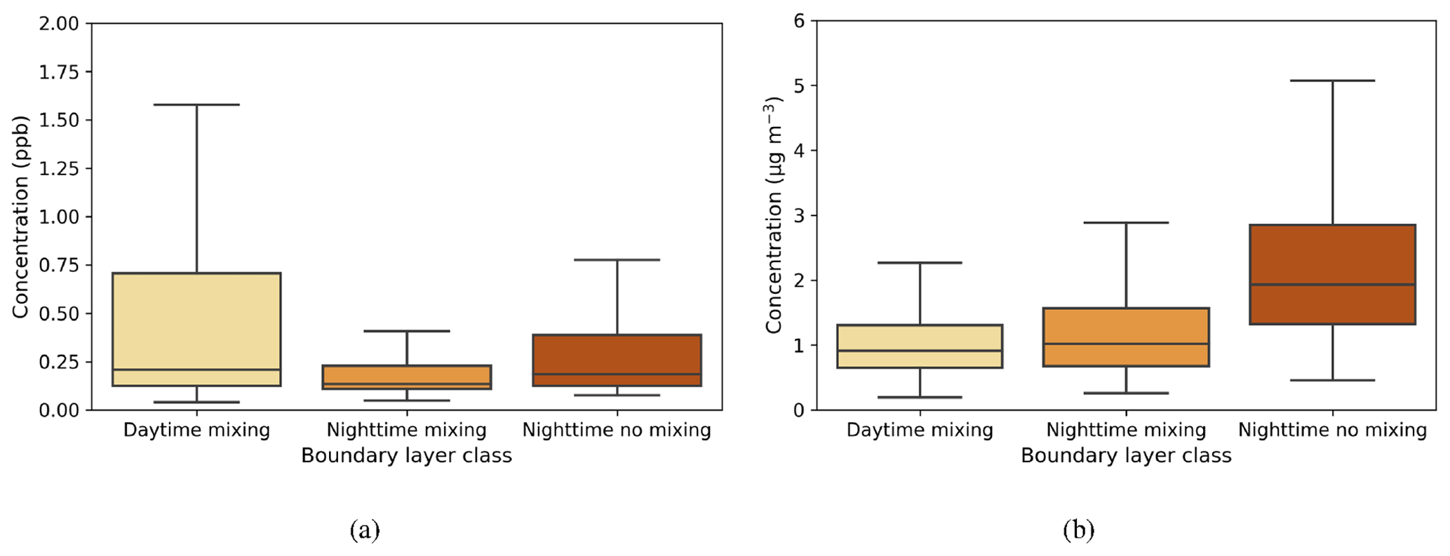
Figure A1Box-and-whisker plots of hourly median values for three boundary layer conditions for (a) SO2 (ppb) and (b) black carbon (µg m−3). The central line in the boxes indicates the median, and the bottom and top lines of the boxes indicate the 25th and 75th percentiles. The whiskers mark the most extreme data points that are not considered to be outliers.
Table A1Summary of the technical specifications of the Halo Streamline Doppler lidar.
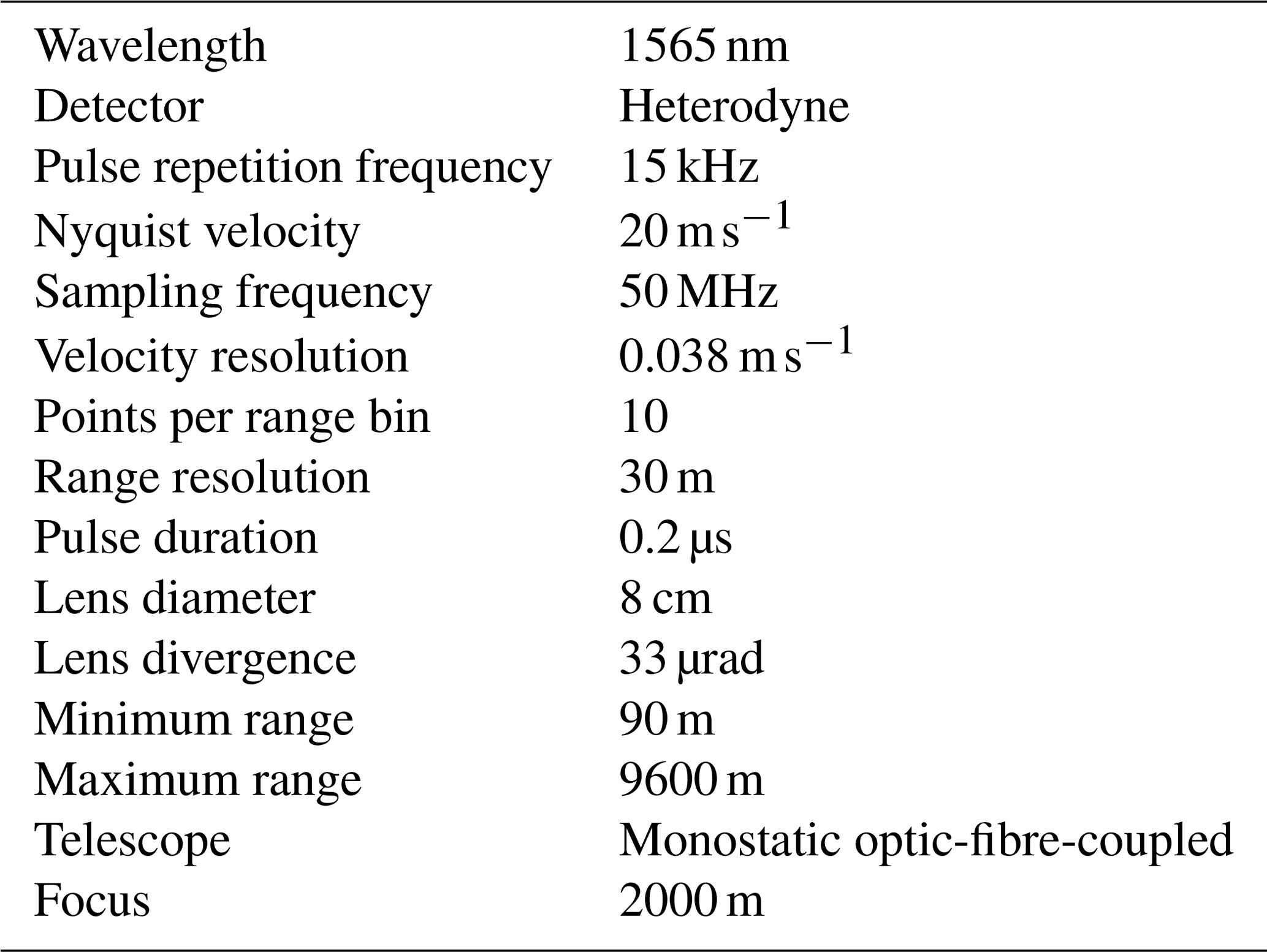
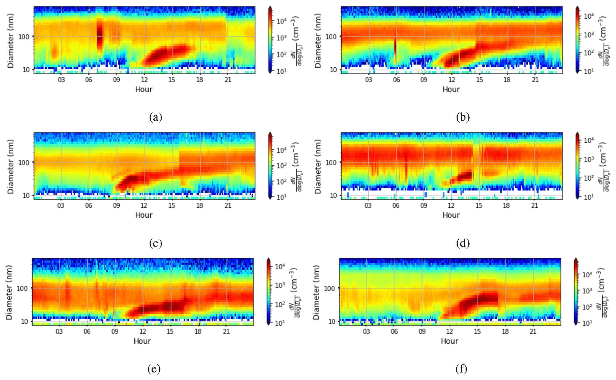
Figure B1Aerosol particle size distribution measured at the surface (the colour indicates the concentration in cm−3) on (a) 23 March 2018, (b) 20 April 2018, (c) 7 May 2018, (d) 13 August 2018, (e) 6 November 2018, and (f) 13 February 2019. For all figures, the time axis is local time (hours UTC+4). Visually estimated aerosol particle growth rates from the figures are (a) 6.7 nm h−1, (b) 6.7 nm h−1, (c) 10 nm h−1, (d) 5 nm h−1, (e) 2.5 nm h−1, and (f) 10 nm h−1.

Figure C1Shallow-boundary-layer case on 21 February 2018. (a) Time–height plot of dissipation rate of turbulent kinetic energy, ϵ; (b) SO2 concentration (ppb) measured at the surface; (c) aerosol particle size distribution measured at the surface (the colour indicates the concentration in cm−3); and time–height plots of (d) wind speed, (e) wind direction, and (f) attenuated backscatter coefficient. For all panels, the time axis is local time (hours UTC+4). The measurements in panels (a, d, e, and f) were obtained from the HALO Doppler lidar.
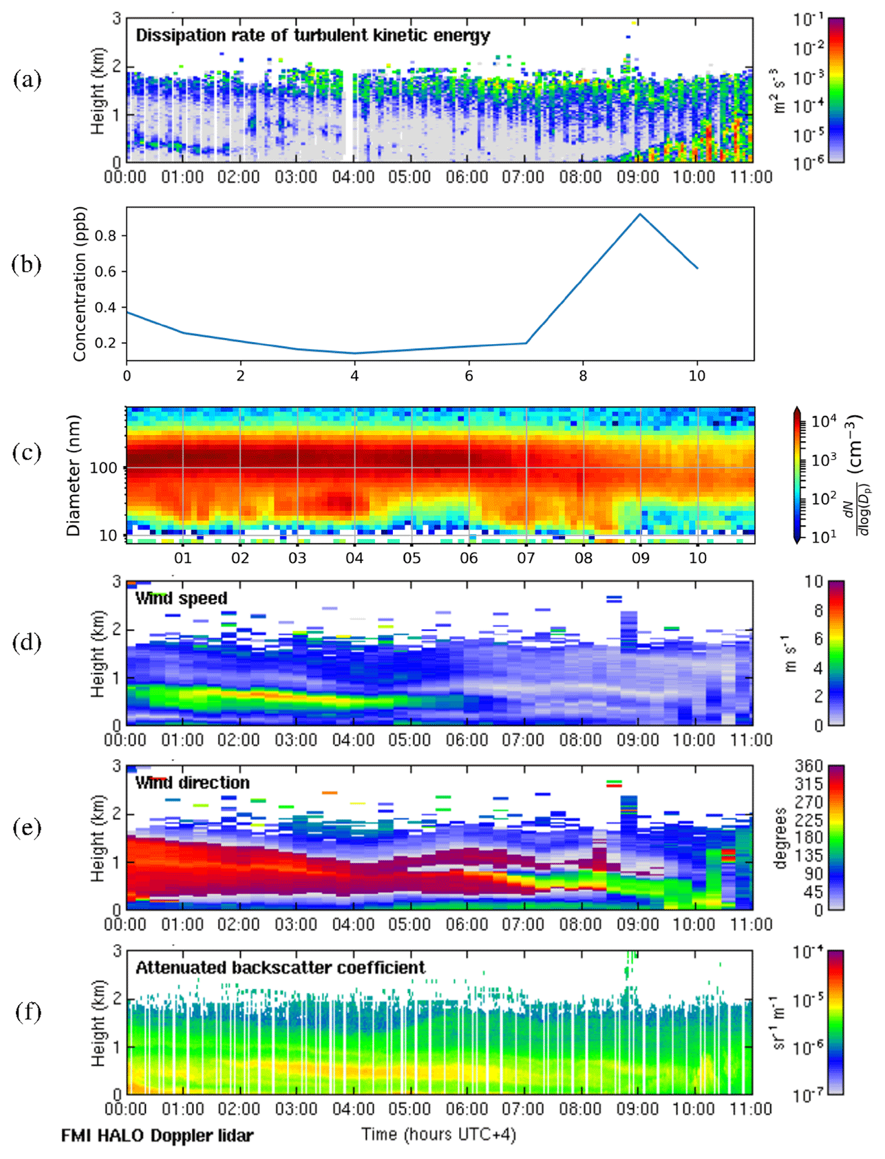
Figure D1Deep-boundary-layer case with stagnant residual layer on 8 May 2018. (a) Time–height plot of dissipation rate of turbulent kinetic energy, ϵ; (b) SO2 concentration (ppb) measured at the surface; (c) aerosol particle size distribution measured at the surface (the colour indicates the concentration in cm−3); and time–height plots of (d) wind speed, (e) wind direction, and (f) attenuated backscatter coefficient. For all panels, the time axis is local time (hours UTC+4). The measurements in panels (a, d, e, and f) were obtained from the HALO Doppler lidar.
The data used in this work are available upon request.
JK, EOC, AH, and EA planned the structure. JK, JB, and HL were responsible for the measurement data. JK, JB, EOC, MA, and UM processed the data. JK, HL, EOC, MA, and UM performed the data analysis. JK, EOC, HL, MA, and UM wrote the paper. All the co-authors were involved in the interpretation of the results and paper editing.
The contact author has declared that neither they nor their co-authors have any competing interests.
Any opinions, findings, and conclusions or recommendations expressed in this material are those of the author(s) and do not necessarily reflect the views of the National Center of Meteorology, Abu Dhabi, UAE, funder of the research.
Copernicus Publications remains neutral with regard to jurisdictional claims in published maps and institutional affiliations.
This work was supported by the National Center of Meteorology, Abu Dhabi, UAE, under the UAE Research Program for Rain Enhancement Science. We would also like to thank Timo Anttila, Siddharth Tampi, and Farah Abdi for providing on-site technical support.
This research has been supported by the Maj and Tor Nessling Foundation (grant no. 202000254) and the Academy of Finland Flagship (grant no. 337552).
This paper was edited by Ottmar Möhler and reviewed by two anonymous referees.
Aalto, P., Hämeri, K., Becker, E., Weber, R., Salm, J., Mäkelä, J. M., Hoell, C., O'Dowd, C. D., Hansson, H.-C., Väkevä, M., Koponen, I. K., Buzorius, G., and Kulmala, M.: Physical characterization of aerosol particles during nucleation events, Tellus B, 53, 344–358, 2001. a
Albrecht, B. A.: Aerosols, cloud microphysics, and fractional cloudiness, Science, 245, 1227–1230, 1989. a
Al Katheeri, E., Al Jallad, F., and Al Omar, M.: Assessment of gaseous and particulate pollutants in the ambient air in Al Mirfa City, United Arab Emirates, Journal of Environmental Protection, 3, 640–647, 2012. a
Arnott, W. P., Hamasha, K., Moosmüller, H., Sheridan, P. J., and Ogren, J. A.: Towards aerosol light-absorption measurements with a 7-wavelength aethalometer: Evaluation with a photoacoustic instrument and 3-wavelength nephelometer, Aerosol Sci. Tech., 39, 17–29, 2005. a
Aurela, M., Saarikoski, S., Timonen, H., Aalto, P., Keronen, P., Saarnio, K., Teinilä, K., Kulmala, M., and Hillamo, R.: Carbonaceous aerosol at a forested and an urban background site in Southern Finland, Atmos. Environ., 45, 1394–1401, 2011. a
Aurela, M., Beukes, J. P., Van Zyl, P., Vakkari, V., Teinilä, K., Saarikoski, S., and Laakso, L.: The composition of ambient and fresh biomass burning aerosols at a savannah site, South Africa, S. Afr. J. Sci., 112, 1–8, 2016. a
Baltensperger, U., Barrie, L., Fröhlich, C., Gras, J., Jäger, H., Jennings, S. G., Li, S.-M., Ogren, J. A., Wiedensohler, A., Wehrli, C., and Wilson, J.: WMO/GAW Aerosol Measurement Procedures, Guidelines and Recommendations, WMO/GAW, 67 pp., 2003. a
Bauer, J. J., Yu, X.-Y., Cary, R., Laulainen, N., and Berkowitz, C.: Characterization of the sunset semi-continuous carbon aerosol analyzer, J. Air Waste Manage., 59, 826–833, 2009. a
Birch, M. E. and Cary, R. A.: Elemental carbon-based method for monitoring occupational exposures to particulate diesel exhaust, Aerosol Sci. Tech., 25, 221–241, 1996. a
Brus, D., Gustafsson, J., Vakkari, V., Kemppinen, O., de Boer, G., and Hirsikko, A.: Measurement report: Properties of aerosol and gases in the vertical profile during the LAPSE-RATE campaign, Atmos. Chem. Phys., 21, 517–533, https://doi.org/10.5194/acp-21-517-2021, 2021. a
Buchhorn, M., Smets, B., Bertels, L., Lesiv, M., Tsendbazar, N.-E., Masiliunas, D., Linlin, L., Herold, M., and Fritz, S.: Copernicus Global Land Service: Land Cover 100m: Collection 3: epoch 2019: Globe (Version V3.0.1), Zenodo [Data set], https://doi.org/10.5281/zenodo.3939050, 2020. a
Cavalli, F., Viana, M., Yttri, K. E., Genberg, J., and Putaud, J.-P.: Toward a standardised thermal-optical protocol for measuring atmospheric organic and elemental carbon: the EUSAAR protocol, Atmos. Meas. Tech., 3, 79–89, https://doi.org/10.5194/amt-3-79-2010, 2010. a, b
Chan, E. A., Gantt, B., and McDow, S.: The reduction of summer sulfate and switch from summertime to wintertime PM2.5 concentration maxima in the United States, Atmos. Environ., 175, 25–32, 2018. a
Cheung, H. C., Chou, C. C.-K., Lee, C. S. L., Kuo, W.-C., and Chang, S.-C.: Hygroscopic properties and cloud condensation nuclei activity of atmospheric aerosols under the influences of Asian continental outflow and new particle formation at a coastal site in eastern Asia, Atmos. Chem. Phys., 20, 5911–5922, https://doi.org/10.5194/acp-20-5911-2020, 2020. a
Dave, P., Bhushan, M., and Venkataraman, C.: Aerosols cause intraseasonal short-term suppression of Indian monsoon rainfall, Sci. Rep.-UK, 7, 1–12, 2017. a
Dusek, U., Frank, G. P., Hildebrandt, L., Curtius, J., Schneider, J., Walter, S., Chand, D., Drewnick, F., Hings, S., Jung, D., Borrmann, S., and Andreae, M. O.: Size matters more than chemistry for cloud-nucleating ability of aerosol particles, Science, 312, 1375–1378, 2006. a, b
Fan, J., Rosenfeld, D., Zhang, Y., Giangrande, S. E., Li, Z., Machado, L. A. T., Martin, S. T., Yang, Y., Wang, J., Artaxo, P., Barbosa, H. M. J., Braga, R. C., Comstock, J. M., Feng, Z., Gao, W., Gomes, H. B., Mei, F., Pöhlker, C., Pöhlker, M. L., Pöschl, U., and de Souza, R. A. F.: Substantial convection and precipitation enhancements by ultrafine aerosol particles, Science, 359, 411–418, 2018. a
Filioglou, M., Giannakaki, E., Backman, J., Kesti, J., Hirsikko, A., Engelmann, R., O'Connor, E., Leskinen, J. T. T., Shang, X., Korhonen, H., Lihavainen, H., Romakkaniemi, S., and Komppula, M.: Optical and geometrical aerosol particle properties over the United Arab Emirates, Atmos. Chem. Phys., 20, 8909–8922, https://doi.org/10.5194/acp-20-8909-2020, 2020. a, b, c
Fitzgerald, J. W., Hoppel, W. A., and Vietti, M. A.: The size and scattering coefficient of urban aerosol particles at Washington, DC as a function of relative humidity, J. Atmos. Sci., 39, 1838–1852, 1982. a
Giechaskiel, B., Ntziachristos, L., and Samaras, Z.: Effect of ejector dilutors on measurements of automotive exhaust gas aerosol size distributions, Meas. Sci. Technol., 20, 045703, https://doi.org/0.1088/0957-0233/20/4/045703, 2009. a
Größ, J., Hamed, A., Sonntag, A., Spindler, G., Manninen, H. E., Nieminen, T., Kulmala, M., Hõrrak, U., Plass-Dülmer, C., Wiedensohler, A., and Birmili, W.: Atmospheric new particle formation at the research station Melpitz, Germany: connection with gaseous precursors and meteorological parameters, Atmos. Chem. Phys., 18, 1835–1861, https://doi.org/10.5194/acp-18-1835-2018, 2018. a
Hakala, S., Alghamdi, M. A., Paasonen, P., Vakkari, V., Khoder, M. I., Neitola, K., Dada, L., Abdelmaksoud, A. S., Al-Jeelani, H., Shabbaj, I. I., Almehmadi, F. M., Sundström, A.-M., Lihavainen, H., Kerminen, V.-M., Kontkanen, J., Kulmala, M., Hussein, T., and Hyvärinen, A.-P.: New particle formation, growth and apparent shrinkage at a rural background site in western Saudi Arabia, Atmos. Chem. Phys., 19, 10537–10555, https://doi.org/10.5194/acp-19-10537-2019, 2019. a
Hitzenberger, R., Berner, A., Dusek, U., and Alabashi, R.: Humidity-dependent growth of size-segregated aerosol samples, Aerosol Sci. Tech., 27, 116–130, 1997. a, b
Hudson, J. G. and Da, X.: Volatility and size of cloud condensation nuclei, J. Geophys. Res.-Atmos., 101, 4435–4442, 1996. a
Hung, H.-M., Lu, W.-J., Chen, W.-N., Chang, C.-C., Chou, C. C.-K., and Lin, P.-H.: Enhancement of the hygroscopicity parameter kappa of rural aerosols in northern Taiwan by anthropogenic emissions, Atmos. Environ., 84, 78–87, 2014. a
IPCC: Climate Change 2013: The Physical Science Basis, in: Contribution of Working Group I to the Fifth Assessment Report of the Intergovernmental Panel on Climate Change, edited by: Stocker, T. F., Qin, D., Plattner, G.-K., Tignor, M., Allen, S. K., Boschung, J., Nauels, A., Xia, Y., Bex, V., and Midgley, P. M., Cambridge University Press, Cambridge, UK and New York, NY, USA, 1535 pp., available at: https://www.ipcc.ch/report/ar5/wg1/ (last access: 5 January 2022), 2013. a, b, c
Jaatinen, A., Romakkaniemi, S., Anttila, T., Hyvärinen, A.-P., Hao, L.-Q., Kortelainen, A., Miettinen, P., Mikkonen, S., Smith, J. N., Virtanen, A., and Laaksonen, A.: The third Pallas Cloud Experiment: Consistency between the aerosol hygroscopic growth and CCN activity, Boreal Environ. Res., 19, 368–382, 2014. a
Jiang, H., Xue, H., Teller, A., Feingold, G., and Levin, Z.: Aerosol effects on the lifetime of shallow cumulus, Geophys. Res. Lett., 33, L14806, https://doi.org/10.1029/2006GL026024, 2006. a
Jokinen, V. and Mäkelä, J. M.: Closed-loop arrangement with critical orifice for DMA sheath/excess flow system, J. Aerosol Sci., 28, 643–648, 1997. a
Junge, C. and McLaren, E.: Relationship of cloud nuclei spectra to aerosol size distribution and composition, J. Atmos. Sci., 28, 382–390, 1971. a
Köhler, H.: The nucleus in and the growth of hygroscopic droplets, T. Faraday Soc., 32, 1152–1161, 1936. a
Komppula, B., Waldén, J., Lusa, K., Kyllönen, K., Saari, H., Vestenius, M., Salmi, J., and Latikka, J.: Ilmanlaadun mittausohje 2017, available at: http://hdl.handle.net/10138/228440 (last access: 5 January 2022), 2017. a
Kulmala, M., Laakso, L., Lehtinen, K. E. J., Riipinen, I., Dal Maso, M., Anttila, T., Kerminen, V.-M., Hõrrak, U., Vana, M., and Tammet, H.: Initial steps of aerosol growth, Atmos. Chem. Phys., 4, 2553–2560, https://doi.org/10.5194/acp-4-2553-2004, 2004. a, b
Laakso, L., Vakkari, V., Virkkula, A., Laakso, H., Backman, J., Kulmala, M., Beukes, J. P., van Zyl, P. G., Tiitta, P., Josipovic, M., Pienaar, J. J., Chiloane, K., Gilardoni, S., Vignati, E., Wiedensohler, A., Tuch, T., Birmili, W., Piketh, S., Collett, K., Fourie, G. D., Komppula, M., Lihavainen, H., de Leeuw, G., and Kerminen, V.-M.: South African EUCAARI measurements: seasonal variation of trace gases and aerosol optical properties, Atmos. Chem. Phys., 12, 1847–1864, https://doi.org/10.5194/acp-12-1847-2012, 2012. a
Lampilahti, J., Leino, K., Manninen, A., Poutanen, P., Franck, A., Peltola, M., Hietala, P., Beck, L., Dada, L., Quéléver, L., Öhrnberg, R., Zhou, Y., Ekblom, M., Vakkari, V., Zilitinkevich, S., Kerminen, V.-M., Petäjä, T., and Kulmala, M.: Aerosol particle formation in the upper residual layer, Atmos. Chem. Phys., 21, 7901–7915, https://doi.org/10.5194/acp-21-7901-2021, 2021. a
Lihavainen, H., Alghamdi, M. A., Hyvärinen, A.-P., Hussein, T., Aaltonen, V., Abdelmaksoud, A. S., Al-Jeelani, H., Almazroui, M., Almehmadi, F. M., Al Zawad, F. M., Hakala, J., Khoder, M., Neitola, K., Petäjä, T., Shabbaj, I. I., and Hämeri, K.: Aerosols physical properties at Hada Al Sham, western Saudi Arabia, Atmos. Environ., 135, 109–117, 2016. a, b, c, d
Manninen, A. J., Marke, T., Tuononen, M., and O'Connor, E. J.: Atmospheric boundary layer classification with Doppler lidar, J. Geophys. Res.-Atmos., 123, 8172–8189, 2018. a
Manninen, A. J., O'Connor, E. J., Vakkari, V., and Petäjä, T.: A generalised background correction algorithm for a Halo Doppler lidar and its application to data from Finland, Atmos. Meas. Tech., 9, 817–827, https://doi.org/10.5194/amt-9-817-2016, 2016. a
Marke, T., Crewell, S., Schemann, V., Schween, J. H., and Tuononen, M.: Long-Term Observations and High-Resolution Modeling of Midlatitude Nocturnal Boundary Layer Processes Connected to Low-Level Jets, J. Appl. Meteorol. Clim., 57, 1155–1170, https://doi.org/10.1175/JAMC-D-17-0341.1, 2018. a
O'Connor, E. J., Illingworth, A. J., Brooks, I. M., Westbrook, C. D., Hogan, R. J., Davies, F., and Brooks, B. J.: A method for estimating the turbulent kinetic energy dissipation rate from a vertically pointing Doppler lidar, and independent evaluation from balloon-borne in situ measurements, J. Atmos. Ocean. Tech., 27, 1652–1664, 2010. a, b
Päschke, E., Leinweber, R., and Lehmann, V.: An assessment of the performance of a 1.5 µm Doppler lidar for operational vertical wind profiling based on a 1-year trial, Atmos. Meas. Tech., 8, 2251–2266, https://doi.org/10.5194/amt-8-2251-2015, 2015. a
Pearson, G., Davies, F., and Collier, C.: An analysis of the performance of the UFAM pulsed Doppler lidar for observing the boundary layer, J. Atmos. Ocean. Tech., 26, 240–250, 2009. a
Pentikäinen, P., O'Connor, E. J., Manninen, A. J., and Ortiz-Amezcua, P.: Methodology for deriving the telescope focus function and its uncertainty for a heterodyne pulsed Doppler lidar, Atmos. Meas. Tech., 13, 2849–2863, https://doi.org/10.5194/amt-13-2849-2020, 2020. a
Petters, M. D. and Kreidenweis, S. M.: A single parameter representation of hygroscopic growth and cloud condensation nucleus activity, Atmos. Chem. Phys., 7, 1961–1971, https://doi.org/10.5194/acp-7-1961-2007, 2007. a, b
Ramanathan, V., Crutzen, P. J., Kiehl, J. T., and Rosenfeld, D.: Aerosols, climate, and the hydrological cycle, Science, 294, 2119–2124, 2001. a
Roberts, G. C. and Nenes, A.: A continuous-flow streamwise thermal-gradient CCN chamber for atmospheric measurements, Aerosol Sci. Tech., 39, 206–221, 2005. a
Rosenfeld, D., Zhu, Y., Wang, M., Zheng, Y., Goren, T., and Yu, S.: Aerosol-driven droplet concentrations dominate coverage and water of oceanic low-level clouds, Science, 363, 6427, https://doi.org/10.1126/science.aav0566, 2019. a
Rye, B. J. and Hardesty, R. M.: Discrete spectral peak estimation in incoherent backscatter heterodyne lidar. I: Spectral accumulation and the Cramer-Rao lower bound, IEEE T. Geosci. Remote, 31, 16–27, 1993. a
Sarangi, B., Ramachandran, S., Rajesh, T., and Dhaker, V. K.: Black carbon linked aerosol hygroscopic growth: Size and mixing state are crucial, Atmos. Environ., 200, 110–118, 2019. a, b
Saxena, P., Hildemann, L. M., McMurry, P. H., and Seinfeld, J. H.: Organics alter hygroscopic behavior of atmospheric particles, J. Geophys. Res.-Atmos., 100, 18755–18770, 1995. a
Semeniuk, T. A., Bruintjes, R. T., Salazar, V., Breed, D. W., Jensen, T. L., and Buseck, P. R.: Individual aerosol particles in ambient and updraft conditions below convective cloud bases in the Oman mountain region, J. Geophys. Res.-Atmos., 119, 2511–2528, 2014. a
Semeniuk, T. A., Bruintjes, R., Salazar, V., Breed, D., Jensen, T., and Buseck, P. R.: Processing of aerosol particles within the Habshan pollution plume, J. Geophys. Res.-Atmos., 120, 1996–2012, 2015. a
Svenningsson, B., Hansson, H.-C., Wiedensohler, A., Noone, K., Ogren, J., Hallberg, A., and Colvile, R.: Hygroscopic growth of aerosol particles and its influence on nucleation scavenging in cloud: Experimental results from Kleiner Feldberg, in: The Kleiner Feldberg Cloud Experiment 1990, Springer, 129–152, https://doi.org/10.1007/978-94-011-0313-8 7, 1994. a
Turpin, B. J. and Huntzicker, J. J.: Identification of secondary organic aerosol episodes and quantitation of primary and secondary organic aerosol concentrations during SCAQS, Atmos. Environ., 29, 3527–3544, 1995. a
Vakkari, V., Beukes, J. P., Laakso, H., Mabaso, D., Pienaar, J. J., Kulmala, M., and Laakso, L.: Long-term observations of aerosol size distributions in semi-clean and polluted savannah in South Africa, Atmos. Chem. Phys., 13, 1751–1770, https://doi.org/10.5194/acp-13-1751-2013, 2013. a
Vakkari, V., Manninen, A. J., O'Connor, E. J., Schween, J. H., van Zyl, P. G., and Marinou, E.: A novel post-processing algorithm for Halo Doppler lidars, Atmos. Meas. Tech., 12, 839–852, https://doi.org/10.5194/amt-12-839-2019, 2019. a
Virkkula, A., Mäkelä, T., Hillamo, R., Yli-Tuomi, T., Hirsikko, A., Hämeri, K., and Koponen, I. K.: A simple procedure for correcting loading effects of aethalometer data, J. Air Waste Manage., 57, 1214–1222, 2007. a
Watson, J. G., Chow, J. C., and Chen, L.-W. A.: Summary of organic and elemental carbon/black carbon analysis methods and intercomparisons, Aerosol Air Qual. Res., 5, 65–102, 2005. a
Wehbe, Y. and Temimi, M.: A Remote Sensing-Based Assessment of Water Resources in the Arabian Peninsula, Remote Sens.-Basel, 13, 247, https://doi.org/10.3390/rs13020247, 2021. a
Wehbe, Y., Ghebreyesus, D., Temimi, M., Milewski, A., and Al Mandous, A.: Assessment of the consistency among global precipitation products over the United Arab Emirates, J. Hydrol. Reg. Stud., 12, 122–135, 2017. a
Wehbe, Y., Temimi, M., Ghebreyesus, D. T., Milewski, A., Norouzi, H., and Ibrahim, E.: Consistency of precipitation products over the Arabian Peninsula and interactions with soil moisture and water storage, Hydrolog. Sci. J., 63, 408–425, 2018. a
Wehbe, Y., Temimi, M., Weston, M., Chaouch, N., Branch, O., Schwitalla, T., Wulfmeyer, V., Zhan, X., Liu, J., and Al Mandous, A.: Analysis of an extreme weather event in a hyper-arid region using WRF-Hydro coupling, station, and satellite data, Nat. Hazards Earth Syst. Sci., 19, 1129–1149, https://doi.org/10.5194/nhess-19-1129-2019, 2019. a
Wehbe, Y., Temimi, M., and Adler, R. F.: Enhancing precipitation estimates through the fusion of weather radar, satellite retrievals, and surface parameters, Remote Sens.-Basel, 12, 1342, https://doi.org/10.3390/rs12081342, 2020. a
Wiedensohler, A., Birmili, W., Nowak, A., Sonntag, A., Weinhold, K., Merkel, M., Wehner, B., Tuch, T., Pfeifer, S., Fiebig, M., Fjäraa, A. M., Asmi, E., Sellegri, K., Depuy, R., Venzac, H., Villani, P., Laj, P., Aalto, P., Ogren, J. A., Swietlicki, E., Williams, P., Roldin, P., Quincey, P., Hüglin, C., Fierz-Schmidhauser, R., Gysel, M., Weingartner, E., Riccobono, F., Santos, S., Grüning, C., Faloon, K., Beddows, D., Harrison, R., Monahan, C., Jennings, S. G., O'Dowd, C. D., Marinoni, A., Horn, H.-G., Keck, L., Jiang, J., Scheckman, J., McMurry, P. H., Deng, Z., Zhao, C. S., Moerman, M., Henzing, B., de Leeuw, G., Löschau, G., and Bastian, S.: Mobility particle size spectrometers: harmonization of technical standards and data structure to facilitate high quality long-term observations of atmospheric particle number size distributions, Atmos. Meas. Tech., 5, 657–685, https://doi.org/10.5194/amt-5-657-2012, 2012. a
Winklmayr, W., Reischl, G. P., Lindner, A. O., and Berner, A.: A new electromobility spectrometer for the measurement of aerosol size distributions in the size range from 1 to 1000 nm, J. Aerosol Sci., 22, 289–296, 1991. a
Wu, W. S. and Wang, T.: On the performance of a semi-continuous PM2.5 sulphate and nitrate instrument under high loadings of particulate and sulphur dioxide, Atmos. Environ., 41, 5442–5451, 2007. a
Ye, X., Tang, C., Yin, Z., Chen, J., Ma, Z., Kong, L., Yang, X., Gao, W., and Geng, F.: Hygroscopic growth of urban aerosol particles during the 2009 Mirage-Shanghai Campaign, Atmos. Environ., 64, 263–269, 2013. a