the Creative Commons Attribution 4.0 License.
the Creative Commons Attribution 4.0 License.
 | 11 Mar 2022
Sensitivity of low-level clouds and precipitation to anthropogenic aerosol emission in southern West Africa: a DACCIWA case study
Adrien Deroubaix
Laurent Menut
Cyrille Flamant
Peter Knippertz
Andreas H. Fink
Anneke Batenburg
Joel Brito
Cyrielle Denjean
Cheikh Dione
Régis Dupuy
Valerian Hahn
Norbert Kalthoff
Fabienne Lohou
Alfons Schwarzenboeck
Guillaume Siour
Paolo Tuccella
Christiane Voigt
During the West African summer monsoon, pollutants emitted in urbanized coastal areas modify cloud cover and precipitation patterns. The Dynamics-Aerosol-Chemistry-Cloud Interactions in West Africa (DACCIWA) field campaign provided numerous aircraft-based and ground-based observations, which are used here to evaluate two experiments made with the coupled WRF–CHIMERE model, integrating both the direct and indirect aerosol effect on meteorology. During one well-documented week (1–7 July 2016), the impacts of anthropogenic aerosols on the diurnal cycle of low-level clouds and precipitation are analyzed in detail using high and moderate intensity of anthropogenic emissions in the experiments. Over the continent and close to major anthropogenic emission sources, the breakup time of low-level clouds is delayed by 1 hour, and the daily precipitation rate decreased by 7.5 % with the enhanced anthropogenic emission experiment (with high aerosol load). Despite the small modifications on daily average of low-level cloud cover (+2.6 %) with high aerosol load compared to moderate, there is an increase by more than 20 % from 14:00 to 22:00 UTC on hourly average. Moreover, modifications of the modeled low-level cloud and precipitation rate occur far from the major anthropogenic emission sources, to the south over the ocean and to the north up to 11∘ N. The present study adds evidence to recent findings that enhanced pollution levels in West Africa may reduce precipitation.
- Article
(13846 KB) - Full-text XML
- BibTeX
- EndNote


In southern West Africa (SWA), the population is rapidly increasing, driving up anthropogenic emissions (AE) (Liousse et al., 2014). During the West African monsoon (WAM) period (June–September), in addition to local pollution emissions, aerosols from two remote sources are transported toward the Guinean coast, namely mineral dust from the north and biomass burning aerosol (BBA) from Central Africa (e.g., Flamant et al., 2018a). These different sources contribute to the high aerosol load over the SWA and have deleterious human health impacts (Bauer et al., 2019).
Depending on their optical and chemical properties, aerosols influence the local meteorology through direct (and semi-direct) effects via the absorption and scattering of radiation, and via hygroscopic aerosol enhancing cloud droplet number concentrations, thereby decreasing droplet sizes (e.g., Haywood and Boucher, 2000; Carslaw et al., 2010). These effects account for modifications in the meteorology especially in the boundary layer, which in turn affect pollution transport and washout (Thompson and Eidhammer, 2014; Baklanov et al., 2017). An adequate representation of these effects is critical for general circulation models (Fan et al., 2016; Seinfeld et al., 2016), especially over West Africa, where clouds in the lowermost troposphere are not well reproduced during the WAM season (Hannak et al., 2017).
The latest generation of numerical weather prediction models integrates the aerosol effects on meteorology (Baklanov et al., 2014). Over Africa, Menut et al. (2019) have shown – with the online coupled WRF–CHIMERE model – that a decrease of anthropogenic emissions along the Guinean coast imposes a northward shift of the monsoonal precipitation associated with an increase of the surface wind speed over arid areas in the Sahel, inducing more mineral dust emissions.
Aerosol transport has complex pathways during the WAM season (Menut et al., 2018). The large amount of biomass burning aerosols in the accumulation mode (i.e., cloud condensation nuclei) transported from Central Africa over the ocean toward the coast of the Guinea Gulf together with the humidity in the monsoon flow impacts cloud microphysics, already reducing the droplet effective radius before reaching the coast (Haslett et al., 2019; Taylor et al., 2019). Upon reaching the highly urbanized regions, these air masses are further loaded with additional aerosols from anthropogenic emissions (Taylor et al., 2019; Denjean et al., 2020). Therefore, the diurnal cycle of winds, low-level clouds (LLC) and precipitation over SWA are impacted by both biomass burning and anthropogenic aerosols (Taylor et al., 2019).
Over continental SWA and during the monsoon period, LLC are formed during the night and break up in the afternoon, however, the variability of the LLC cover is only partly understood, which is mainly due to the lack of measurements in this region (Knippertz et al., 2015a). One of the goals of the recent DACCIWA project (Dynamics-Aerosol-Chemistry-Cloud Interactions in West Africa) was to address this issue, using the important database collected during June and July 2016 (Knippertz et al., 2015b, 2017). The interactions between the nocturnal low-level jet and LLC were studied during the DACCIWA campaign deployed in SWA, using radiosondes, aircraft (Flamant et al., 2018b), and three super-sites (Kalthoff et al., 2018).
During the months of June and July, the maritime air from the Atlantic reaches Savè (Benin), one of the DACCIWA super-sites about 185 km north of the coast, between 16:00 and 21:00 UTC associated with the occurrence of the nocturnal low-level jet and the LLC (Dione et al., 2019; Zouzoua et al., 2021). Between 22:00 and 06:00 UTC, the LLC layer continues it formation, due to an increase of relative humidity (RH) caused by the advection of cold air (Adler et al., 2019; Babić et al., 2019; Lohou et al., 2020). The persistence of LLC has a considerable impact on the energy balance at the surface (Lohou et al., 2020).
In general, three phases of the wind in the lowest troposphere in SWA can be distinguished according to Adler et al. (2017) and Deetz et al. (2018a, b): (i) a phase of low wind speed from 09:00 to 15:00 UTC, referred as “daytime drying”; (ii) an increase of meridional wind when convection decreases in the boundary layer from 16:00 to 02:00 UTC, referred to as “maritime inflow”; and (iii) a subsequent decrease of meridional wind from 03:00 to 08:00 UTC referred as “moist morning”. Moreover, Deroubaix et al. (2019) have shown that pollutants are accumulated along the coast during the “daytime drying” phase and transported inland during the “maritime inflow” phase, which suggests that LLC and precipitation could be especially modified by anthropogenic aerosol during a specific phase.
This article aims at understanding the influence of the anthropogenic aerosol emissions on the diurnal cycle of LLC and precipitation in SWA. The DACCIWA campaign provides a unique chance to analyze and validate online coupled models. This study presents numerical modeling experiments conducted with WRF-CHIMERE in combination with aerosol and cloud observational datasets from the DACCIWA campaign, which are described in Sect. 2. An analysis of the location and intensity of the modeled anthropogenic plumes is given in Sect. 3. The mean state of humidity and wind is presented in Sect. 4. In Sect. 5, we analyze the modifications of LLC and precipitation by the anthropogenic aerosol emissions from the Gulf of Guinea coast to a few hundred of kilometers north, followed by their consequences at the regional scale in Sect. 6. Conclusions appear in Sect. 7.
In this section, we briefly present the coupling of the WRF (Weather Research and Forecast) model and the CHIMERE chemistry-transport model (Sect. 2.1), and the two experiments conducted using two different anthropogenic emission scenarios (Sect. 2.2). We then detail the observational datasets acquired during the DACCIWA campaign used to evaluate the two experiments and analyze LLC and precipitation (Sect. 2.3).
2.1 CHIMERE model and its coupling with WRF
The WRF model is widely used for various meteorological studies at the regional scale (Powers et al., 2017). We use the model in its 3.7.1 version (Skamarock and Klemp, 2008), allowing non-hydrostatic motion to be calculated (Janjic, 2003). The surface layer scheme is the Carlson–Boland viscous sub-layer with the surface physics calculated by the “Noah” land surface model (Ek et al., 2003). The planetary boundary layer (PBL) physics are calculated by the Yonsei University scheme (Hong et al., 2006). We use the scale-aware scheme of convective parameterization proposed by Grell and Freitas (2014) without sub-grid cloud fraction scheme.
Meteorological initial and boundary conditions are provided by the operational analyses produced by the US National Center for Environmental Prediction (operational analyses: ds083.3 dataset, DOI: https://doi.org/10.5065/D65Q4T4Z, National Centers for Environmental Prediction/National Weather Service/NOAA/U.S. Department of Commerce, 2015). These fields are used to nudge hourly fields of pressure, temperature, humidity, and wind in the WRF simulations, with spectral nudging, which has been evaluated for regional models by von Storch et al. (2000). In order to enable the PBL variability to be resolved by WRF, low frequency spectral nudging is used only above the 12th vertical level. This set-up has already been used over SWA by Deroubaix et al. (2018, 2019).
CHIMERE (version 2017) is a regional chemistry-transport model, which is fully described in Menut et al. (2013) and Mailler et al. (2017) for its offline mode. Bessagnet et al. (2004) describe the calculation of gaseous species in the MELCHIOR-2 (reduced) scheme and the aerosol scheme, which takes into account species such as sulfate, nitrate, ammonium, primary organic matter, black carbon, secondary organic aerosols, sea salt, dust, and water. All aerosols are represented using 10 bins, from 40 nm to 40 µm in diameter. Menut et al. (2016) have validated and analyzed aerosol speciation and size distribution as well as the chemical mechanisms used in the CHIMERE model over Europe and North Africa. Boundary conditions at a 6 h time step are taken from the Copernicus Atmosphere Monitoring Service made by the European Centre for Medium-Range Weather Forecasts (Inness et al., 2019) for both experiments. These include the biomass burning aerosols from Central Africa (and mineral dust aerosols from the Sahel–Sahara), thanks to assimilation of aerosol optical depth retrieved from the Moderate Resolution Imaging Spectroradiometer (MODIS) in this dataset (Fig. A1).
The coupled WRF–CHIMERE model integrates the direct (and semi-direct) and indirect effects between CHIMERE and WRF through exchanges via an external coupling software developed primarily for use in the climate community, namely OASIS3-MCT (Craig et al., 2017), at a 10 min time step. Three fields are sent to the radiative scheme of WRF to represent the direct effect: (i) aerosol optical depth, (ii) single scattering albedo, and (iii) asymmetry parameter (Briant et al., 2017). The indirect effect is taken into account thereby transferring four fields of CHIMERE to the microphysics scheme of WRF: (i) aerosol size distribution (the 10 bins used in CHIMERE to simulate the aerosol size distribution are transferred to WRF), (ii) bulk hygroscopicity of internally mixed aerosols (the hygroscopicity is a unique value calculated for each grid point), (iii) ice nuclei, and (iv) deliquesced aerosols (Tuccella et al., 2019). Moreover, the wet scavenging is calculated in CHIMERE using the liquid and frozen precipitation flux, and liquid and frozen hydrometeor mixing ratio.
For the coupled WRF–CHIMERE model, two schemes are mandatory in order to reproduce: (i) the direct effects, which are taken into account through exchanges between the radiative scheme and CHIMERE, the Rapid Radiative Transfer Model for general circulation models with the Monte-Carlo Independent Column Approximation method of random cloud overlap (Mlawer et al., 1997; Iacono et al., 2008); and (ii) the indirect effects, which are accounted for via the aerosol-aware microphysics scheme proposed by Thompson and Eidhammer (2014) taking into account the modifications in lifetime and reflectivity of clouds due to aerosols.
The scheme proposed by Thompson and Eidhammer (2014) is an aerosol-aware cloud microphysics scheme including a parametrization for aerosol activation based on a single mode log-normal distributed aerosol population taken from a climatology. In WRF-CHIMERE, this approach has been replaced by using the aerosol size distribution and composition predicted by CHIMERE and the aerosol activation as cloud water droplet is parameterized following the Abdul-Razzak (2002) approach. Starting from the updraft velocity, aerosol size distribution and composition, Abdul-Razzak (2002) scheme predicts the fraction of activated aerosol within each model section as a function of maximum supersaturation of an adiabatic rising parcel. According to Ghan et al. (1997), the fraction of aerosols activated in each section of CHIMERE size distribution is calculated on a maximum supersaturation determined from a Gaussian spectrum of updraft velocity and internally mixed aerosol properties following a similar method adopted in WRF-Chem (Chapman et al., 2009). Further details may be found in Tuccella et al. (2019).
In WRF-CHIMERE, the aerosol load affects the cloud lifetime and the precipitation because it modifies the autoconversion from cloud water droplet to rain particles, which is based on the scheme of Berry and Reinhardt (1974). Moreover, it is also affected by the radiation absorption from dust or black carbon via the semi-direct effect (Briant et al., 2017). Over West Africa, the high aerosol load makes the integration of aerosol effects an important step towards understanding meteorological feedbacks during the monsoon (Menut et al., 2019).
2.2 Anthropogenic emission experiments
The simulated period runs from 1 to 7 July 2016 (with a spin-up period starting on 23 June), which is entirely included in the post-onset phase of the 2016 WAM defined from 22 June to 20 July 2016 by Knippertz et al. (2017). The 32 vertical levels of WRF from the surface to 50 hPa are projected onto the 20 levels of CHIMERE from the surface up to 200 hPa, which includes 12 levels below 2 km where the LLC are located, this is why spectral nudging is only applied for vertical levels above the 12th level. Simulations are performed at 5 km resolution in order to explicitly resolve convection. The domain extending from 1∘ S to 12∘ N and from 10∘ W to 8∘ E (located in the Greenwich Mean Time) is shifted compared to Deroubaix et al. (2018, 2019) to the south and to the west in order to improve the modeled WAM flux (Fig. 1).
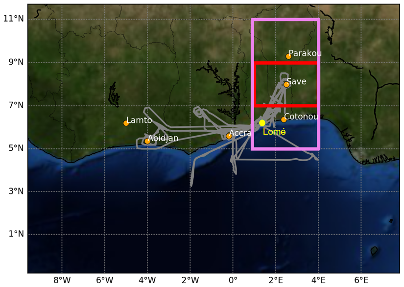
Figure 1Map of the modeling domain with locations of the radiosonde launch sites (orange dots), Lomé airport (yellow dot), and the flight tracks of the three research aircraft during the 1–7 July 2016 period (gray lines). The red and violet rectangles represent the three investigated areas.
The Hemispheric Transport of Air Pollution version 2 (HTAPv2) inventory provides the anthropogenic emission flux (Janssens-Maenhout et al., 2015). This dataset is relevant for the year 2010 and, given that the population is rapidly increasing in this region, it should underestimate the 2016 emissions.
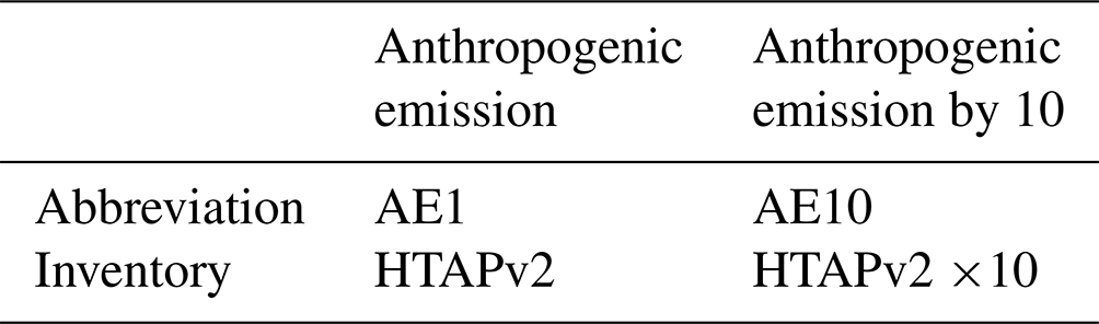
Therefore, two experiments are proposed (Table 1): (i) a simulation with HTAPv2 designed to underestimate anthropogenic emission (AE), which is called AE1, and (ii) a simulation designed to overestimate the AE obtained by multiplying the emissions of HTAPv2 by a factor of 10, called AE10. This factor may seem huge but is not unrealistic, as anthropogenic emissions are estimated to increase very rapidly as “explosive growth” (Liousse et al., 2014).
Table 1Name and corresponding anthropogenic emission inventory of the two WRF-CHIMERE coupled simulations used in this study.
2.3 Measurements in the framework of the DACCIWA project
We use three types of measurements of the DACCIWA campaign: (i) radiosonde measurements, (ii) aircraft measurements, (iii) ground-based measurements at Savè. Ground measurement stations and aircraft trajectories are illustrated in Fig. 1. Additionally, precipitation rate retrieved by the Tropical Rainfall Measuring Mission (TRMM), and aerosol optical depth and liquid water path retrieved by the Moderate Resolution Imaging Spectroradiometer (MODIS), both provided by NASA, and the Spinning Enhanced Visible and Infra-Red Imager (SEVIRI) images provided by EuMetSat and NAScube, are presented.
- i.
We selected six locations of the radiosonde campaign: Lamto and Abidjan in Ivory Coast, Accra in Ghana, Cotonou, Savè and Parakou in Benin (Fig. 1). There were four releases per day at around 00:00, 06:00, 12:00, and 18:00 UTC, and in Savè additional radiosondes were launched every 1.5 to 3 h during intensive observation periods (Kalthoff et al., 2018).
- ii.
The DACCIWA aircraft campaign took place during the period 25 June–14 July 2016, with three research aircraft: a Twin Otter operated by the British Antarctic Survey, an ATR-42 operated by the French “Service des Avions Français Instrumentés pour la Recherche en Environnement”, and a Falcon-20 operated by the German “Deutsches Zentrum für Luft- und Raumfahrt”, based at the Lomé (Togo) airport (Flamant et al., 2018b).
Mass concentrations of four aerosol types are analyzed, namely black carbon (BC), organic carbon (OC), ammonium, and nitrate, as well as two trace gases, CO and NO2, and meteorological variables. We use measurements of a SP2 (Single Particle Soot Photometer) for black carbon, and of a C-ToF-AMS (Compact Time-of-Flight Aerosol Mass Spectrometer) instruments for inorganic and organic aerosol concentration. We compare with modeled aerosol size less than 1 µm, which is compatible to the aerosol instruments used here.
- iii.
At Savè, one of the three super-sites of the DACCIWA project, meteorological measurements were performed. Savè is a village located downstream of several large coastal cities, due to the prevailing low-level southwesterlies during the WAM season. For Savè, priority is given to the CHM15k ceilometer data providing a robust value of the cloud base height (Adler et al., 2019; Dione et al., 2019; Lohou et al., 2020).
In this section, we evaluate the spatial variability of the modeled anthropogenic aerosol concentration in the lowermost troposphere, with a particular focus given to the location and the magnitude of the modeled pollution plumes. We investigate four aerosol types (BC, OC, ammonium, nitrate), which are of prime importance due to their optical and hygroscopic properties (Carslaw et al., 2010). We first analyze the modeled aerosol concentration distributions with observations acquired below 2 km a.m.s.l. (above mean sea level) using all available measurements (Table 2). Secondly, we study in detail a specific flight of the ATR-42 conducted on 6 July (Fig. 2).
Table 2Distribution of observed and modeled aerosol concentrations (in µg m−3) given by first quartile (Q1), median (Q2) and third quartile (Q3) of black carbon (BC), organic carbon (OC), ammonium, and nitrate below 2 km a.m.s.l. (and above 300 m a.m.s.l. to avoid airport areas) using all flights of the DACCIWA campaign during the period 1–7 July 2016. N is the number of samples for the comparison between observations and simulations.
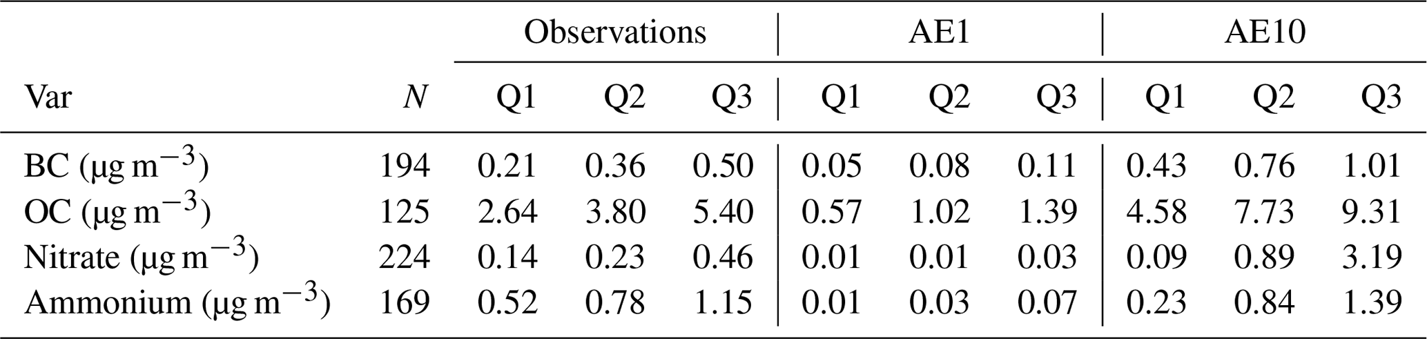
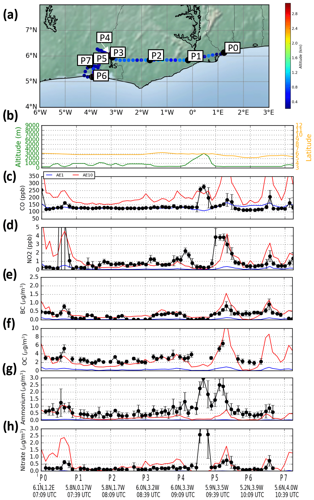
Figure 2(a) Map of the flight spatial trajectory of the ATR-42 research aircraft data on 6 July 2016, and time series composed of seven parts (from the top to the bottom): (b) the altitude (in m a.m.s.l.) with the latitude (in ∘ N); (c–h) the six other panels present the modeled values interpolated along the flight positions for the two experiments, AE1 (blue line) and AE10 (red line), and the 3 min averaged observations (black points and the associated standard deviation with the error bars) of: (c) carbon monoxide (CO in ppb), (d) nitrogen oxides (NO2 in ppb), (e) black carbon (BC in µg m−3), (f) organic carbon (OC in µg m−3), (g) ammonium (in µg m−3), (h) nitrate (in µg m−3). Aerosol concentrations are measured with a cut-off diameter of 1 µm and the modeled concentrations are shown accordingly.
We compare the distribution of the aerosol concentrations (BC, OC, ammonium, nitrate) of the two experiments (AE1 and AE10) with measurements of the three aircraft below 2 km (and above 300 m a.m.s.l. to avoid perturbation close to the airport areas). The number of 3 min averaged observations is about 200 during the studied period, which corresponds to about 10 h of sampling. The modeled concentrations are interpolated along the flight positions with a triple interpolation (bi-linear horizontally, linear vertically, and linear between two time steps).
The observations show that the OC concentration is by far the highest (Q1[OC] > Q3[others]), followed by ammonium, BC, and nitrate (Table 2). The model reproduces that OC concentration is higher than ammonium, BC, and nitrate. For all aerosol types, the observations are between AE1 and AE10. With AE10, NOx concentration is multiplied by 10, but the nitrate and ammonium concentrations are a factor 100 higher from AE1 to AE10. This shows the non-linearity of NOx to nitrate conversion and also a possible misrepresentation in the CHIMERE model, as has already been raised by Petetin et al. (2016). The underestimation of BC and OC by the two experiments could be explained by low emission factors in anthropogenic emission inventories (such as HTAPv2), as shown using in-situ measurement made during the DACCIWA campaign (Keita et al., 2018). We conclude that the range of the modeled aerosol concentration is realistic, and that the AE10 experiment is closer to the observations than AE1.
We select one specific flight in order to evaluate the location of the anthropogenic sources. This flight was performed by the ATR-42 on 6 July from Lomé in Togo (take-off at 07:09 UTC) to Abidjan in Ivory Coast (landing at 10:45 UTC), during the time of day when the boundary layer height over the continent starts to increase, while being typically below 1 km a.m.s.l. in the morning (Kalthoff et al., 2018). This flight is particularly interesting because it was performed mostly below 1 km a.m.s.l., over coastal, forest, and urban areas, and allowed measurements in the vicinity of three major population centers (Lomé, Accra, and Abidjan), with all instruments operating normally (Fig. 2).
The modeled aerosol concentrations are compared to aircraft measurements together with modeled and observed concentrations of CO and NO2 used as proxies of the (incomplete) combustion and of urban areas, respectively. The analysis of the concentrations measured during the flight is separated into eight positions. For this flight, Brito et al. (2018) have decomposed the aerosol concentration measurements into three parts, which correspond to: (i) advecting air mass (close to position P6), (ii) Abidjan plume (between position P5 and P6), and (ii) continental (between position P1 and P4). On average, the continental aerosol concentration was 0.33 µg m−3 for BC, 2.91 µg m−3 for OC, 0.21 µg m−3 for ammonium, and 0.17 µg m−3 for nitrate. A clear enhancement was measured in the Abidjan plume compared to continental aerosol concentrations, while advecting air mass and continental aerosol concentrations were similar (except for OC higher over the continent due to biogenic sources).
From position P0 to P1 (07:09 to 07:39 UTC), the aircraft sampled coastal urban areas between Lomé and Accra. Aerosol concentrations are high for the four studied aerosol types (BC ranges from 0.3 to 0.8 µg m−3, OC from 3 to 5 µg m−3, ammonium from 0.4 to 1.2 µg m−3, and nitrate from 0.1 to 0.5 µg m−3). The observations are closest to the AE10 experiment. We attribute the peak observed at 07:25 UTC to the Accra plume with high CO up to 160 ppb and especially high NO2 up to 17.9 ppb (Fig. 2). This also corresponds to a peak in the time series of BC (0.8 µg m−3), OC (5.2 µg m−3), ammonium (1.2 µg m−3), and nitrate (0.6 µg m−3). The model predicts this peak in better agreement for AE10 than AE1. The AE1 experiment underestimates the concentrations of all aerosols, while AE10 is correct for BC, OC, ammonium, and overestimates nitrate by 1.6 µg m−3 on average.
From position P1 to P4 (07:39 to 09:09 UTC), the aircraft sampled continental background concentrations corresponding to low NO2 and CO (about 1 and 120 ppb, respectively), since it flew over areas of low population density as well as forested areas. The OC and ammonium concentrations remain high (OC about 3.2 µg m−3, ammonium about 0.6 µg m−3), whereas a more pronounced decrease is noticed for BC and nitrate concentrations (BC about 0.3 µg m−3, nitrate from 0.2 µg m−3). The observations are between AE1 and AE10 for BC (AE1 about 0.05 µg m−3 and AE10 about 0.3 µg m−3), OC (AE1 about 0.3 µg m−3 and AE10 about 3.0 µg m−3), and nitrate (AE1 about 0.01 µg m−3 and AE10 about 0.1 µg m−3), while ammonium is underestimated (by 0.3 µg m−3 with AE10).
From position P4 to P5 (09:09 to 09:39 UTC), the aircraft performed a vertical sounding, reaching 3 km, before going back down, measuring an increase of CO (> 250 ppb), ammonium (> 2.8 µg m−3) and nitrate (> 3 µg m−3) associated with low NO2 (< 0.5 ppb), which suggests aged biomass burning air masses, described in detail by Brito et al. (2018) and Haslett et al. (2019). The model does not reproduce this feature in the aerosol concentrations.
From position P5 to P6 (09:39 to 10:39 UTC), the aircraft circled around the city of Abidjan, flying upwind then downwind then upwind again. There is a clear increase of the aerosol concentrations, showing that the aircraft was flying through the city's plume, with high concentrations of CO (> 150 ppb) and NO2 (> 1 ppb), likewise for the four aerosol concentrations studied (BC up to 1 µg m−3, OC up to 6 µg m−3, ammonium up to 2.5 µg m−3, nitrate up to 0.7 µg m−3). The modeled aerosol concentrations increase, showing that this plume is well represented in AE10 with low biases for BC, OC, and nitrate (but ammonium is underestimated by −0.7 µg m−3). AE1 represents this plume with much larger biases.
From position P6 to P7 (09:39 to 10:39 UTC), upwind of Abidjan, another plume of high CO, NO2, BC, ammonium, and nitrate is sampled, which is well reproduced by AE10, also with low biases (for BC up to +0.1 µg m−3, ammonium up to +0.4 µg m−3, nitrate up to +0.01 µg m−3), whereas their counterparts in AE1 are all underestimated.
Overall, the ATR-42 flight on 6 July shows that the location of the urban plumes is well modeled, thus we can infer that the main aerosol sources are also well located. The magnitude of the anthropogenic emission sources is underestimated for the AE1 experiment, and slightly overestimated for the AE10 experiment.
In conclusion, the urban plumes of Accra and Abidjan are well reproduced by the model. The range of modeled aerosol concentrations is realistic for both simulations, although the simulation AE10 is closer to the observations. The two experiments allow investigation of the effect of changes in anthropogenic aerosol emission change on meteorology, as discussed in the following.
We now want to evaluate the modeled meteorology and quantify the sensitivity to the aerosol load described by the two experiments. We select two meteorological variables, namely relative humidity (RH) and wind speed (WS), for which the vertical profiles have already been described by e.g., Deroubaix et al. (2019). We evaluate firstly the averaged vertical profiles using radiosonde measurements, and secondly the variability of these two variables using aircraft measurements.
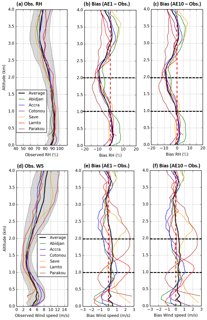
Figure 3Observed mean vertical profiles of wind speed (in m s−1), and relative humidity (RH in %) averaged for all profiles over the period 1–7 July 2016 at Abidjan (green line) and Lamto (red line) in Ivory Coast, Accra in Ghana (blue line), Cotonou (purple line), Savè (orange line) and Parakou (brown line) in Benin. The mean and standard deviation at the six locations are represented by the black line and the gray shading (a, d). WRF-derived variables are interpolated to the radiosonde positions and (b, c; e, f) vertical biases (mod-obs) are presented at each location (colored line) and for the average of the six locations (black line) for the experiments AE1 and AE10.
In the modeled domain, there are six radiosonde sites where balloons were frequently launched (cf. Sect. 2.3), which corresponds to 28 balloon launches in Abidjan, 28 in Accra, 23 in Cotonou, 43 in Savè, 7 in Lamto, and 28 in Parakou. The averages of the observed vertical profiles are presented for each site as well as their mean and standard deviation. We analyze the vertical biases (mod-obs) of the two experiments (Fig. 3).
The observed mean vertical profiles are composed of three vertical parts: (i) from the surface to 1 km a.m.s.l., close to saturation (> 90 %), which is the monsoon layer, (ii) from 1–2 km a.m.s.l., RH close to 90 % and low wind speed, which is a directional shear layer, and (iii) from 2–4 km a.m.s.l., a drier and faster layer compared to below layers, which is a mid-level easterly flow layer, south of the African Easterly Jet core, and for which Parakou and Savè are the closest. These three layers are reproduced by WRF-CHIMERE as already shown by Deroubaix et al. (2019) and Menut et al. (2019).
For all locations, the observed vertical profiles present a decrease of RH from the surface to 3 km a.m.s.l., and for WS, the average is high in the monsoon layer (about 6 m s−1), low in the directional shear layer (about 4 m s−1), and high in the mid-level easterly flow layer (about 8 m s−1). From 2 to 4 km a.m.s.l., the WS observed vertical profile at Parakou and Savè stand out because the wind is higher than at the other locations, being closer to the African Easterly Jet core.
The vertical biases are similar for the two experiments, which shows that the synoptic profiles are only marginally modified by aerosol effects. Similar vertical biases are noticed in all locations as a function of altitude, except for WS at the stations far from the coast (Lamto, Savè, and Parakou). Thus, it is consistent to quantify the bias of the model for the three ranges of altitude described above (Table 3). There is a clear dry bias in both experiments between 1.5 and 2.5 a.m.s.l., which is also present in the data of the Integrated Forecasting System of the European Centre for Medium-range Weather Forecasts (van der Linden et al., 2020).
Table 3Mean biases (mod–obs) of observed and modeled (experiments AE1 and AE10) vertical profiles of relative humidity (RH) and wind speed (WS) over three altitude ranges (i) from the surface to 1 km, (ii) from 1–2 km, (iii) from 2–4 km, using the average of 157 radiosondes launched during the period 1–7 July 2016.
The bias is slightly reduced for RH with AE10 compared to AE1 in the three vertical layers, by 0.21 % between 0 and 1 km a.m.s.l., by 0.24 % between 1 and 2 km a.m.s.l. and 0.05 % between 2 and 4 km a.m.s.l. This suggests an underestimation of vertical mixing with a PBL that is too moist, and a free troposphere above that is too dry. The bias is lower from the surface to 1 km a.m.s.l. than in the above layers. For wind speed, the biases remain similar between AE1 and AE10. Nevertheless, we note that the bias on WS is reduced in Accra and Cotonou in the first kilometer when comparing AE10 to AE1 (Fig. 3).
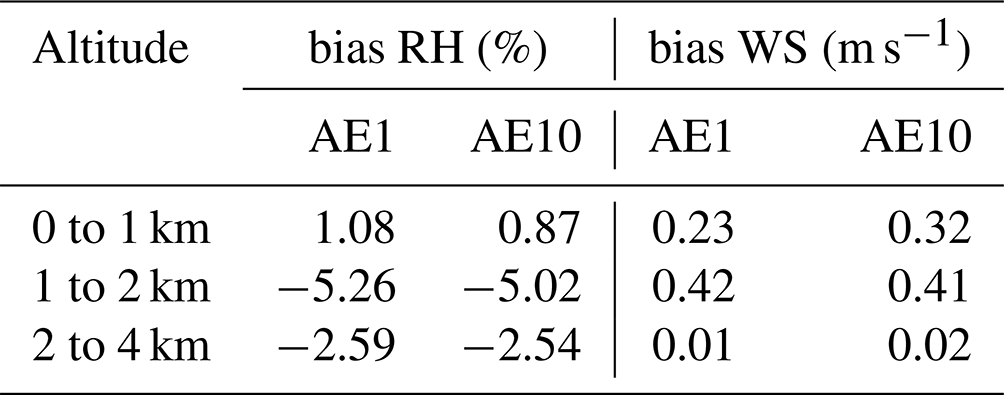
Now, we want to analyze in detail the modeled and observed variability in the lowermost troposphere (< 4 km). We compare 3 min averages of aircraft measurements with the model interpolated to the flight trajectory (with the same methodology as in Sect. 3), using scatter plots (Fig. 4) together with reduced major axis regression fits (Ayers, 2001; Smith, 2009).
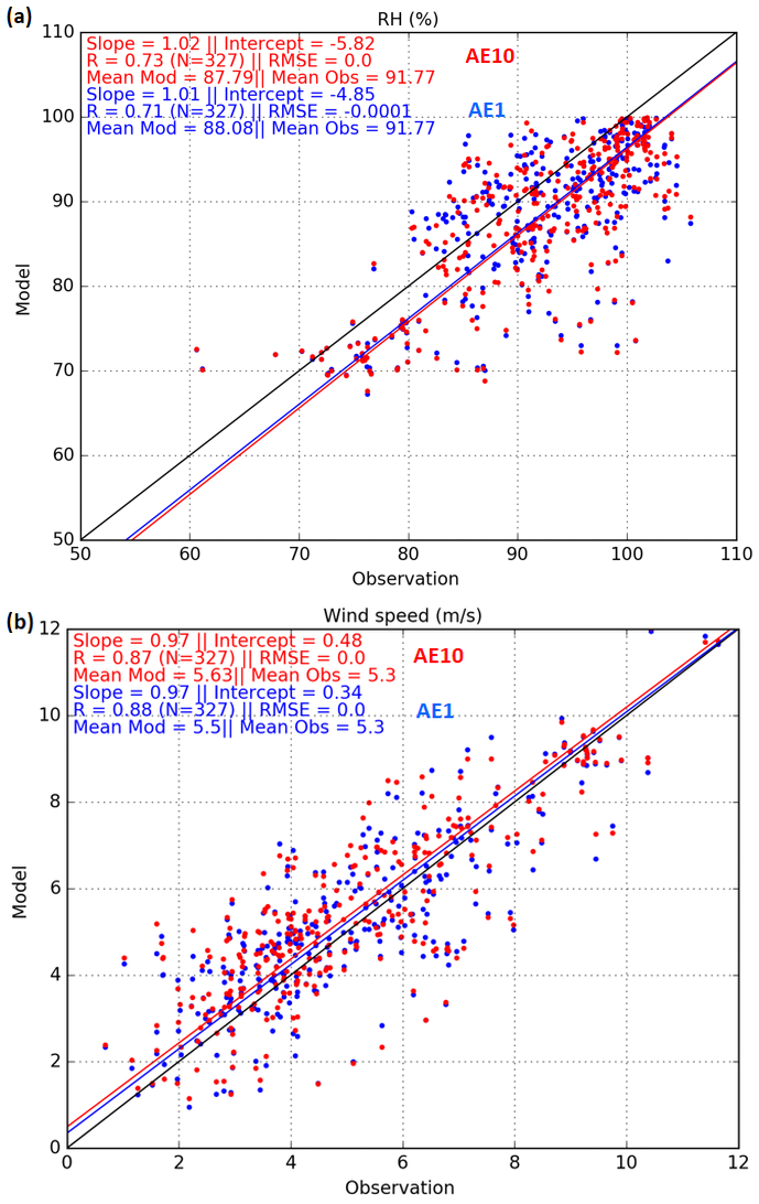
Figure 4Scatter plot of (a) relative humidity (RH) and (b) wind speed (WS) with the 3 min averaged observations against the modeled values interpolated along the flight positions for the two experiments AE1 (in blue) and AE10 (in red) below 4 km a.m.s.l. (and above 300 m a.m.s.l.) using all flights of the DACCIWA campaign during the period 1–7 July 2016. Statistics of a linear regression analysis are given in top left corner of each panel.
While the observed RH may exceed 100 % at times, the modeled values are lower than 100 % (Fig. 4) because cloud water condenses only when the water vapor exceeds a saturation threshold calculated with the polynomial approximation from Flatau et al. (1992). The saturation adjustment is treated by solving the Clausius–Clapeyron equation with the Newton–Raphson interactive scheme (Thompson et al., 2008). On average, for the period 1–7 July, the model underestimates humidity, especially for low humidity (60 %–70 %). The regression coefficients and the slopes of the regression are high and similar for both experiments (R = 0.73 for AE10 and R = 0.71 for AE1; slope of 1.02 for AE1 and of 1.01 for AE10). The wind speed observations range from 1 to 12 m s−1. The model predicts the same range with a positive bias of 0.2 m s−1 for AE1 and 0.33 m s−1 for AE10. The model–observation comparison for wind speed are similar for the two experiments (R = 0.88 for AE1 and R = 0.87 for AE10).
In conclusion, the vertical mean profiles and the range of variability of relative humidity and wind speed are well represented below 4 km a.m.s.l. in the two experiments. There is no clear improvement from AE1 to AE10 for relative humidity and wind speed because differences in the correlation coefficients are less than 0.1 between the two experiments. The mean state of the lowermost troposphere is only marginally modified despite the important difference in the aerosol load between the two experiments, which is normal since an important change in the relative humidity and wind speed by the introduction of the aerosol effects in the coupled model is not expected. However, we expect LLC and precipitation to be more influenced by the large difference in anthropogenic aerosol load between the two experiments.
This section aims at evaluating the sensitivity of the modeled LLC diurnal cycle to the anthropogenic aerosol load differences between the two experiments. We first focus on 5 July 2016 of the DACCIWA campaign, because the three aircraft were flying with a similar flight plan targeting LLC at different times of the day. Second, we study the LLC diurnal cycle during the studied week at the site of Savè in Benin. Finally, we analyze the features of the LLC diurnal cycle most influenced by the anthropogenic aerosol emissions.
On 5 July, the Lomé–Savè transect was flown by the ATR-42 in the morning (from 08:00 to 11:00 UTC), then by the Falcon-20 at noon (from 11:30 to 13:50 UTC), ending with the TO (from 15:50 to 17:50 UTC, which is not presented because it occurred after the LLC breakup time between 15:00 and 16:00 UTC). We compare the liquid water mixing ratio (LWMR, in kg kg−1) measured with 3 min averages and modeled using vertical cross sections along the aircraft trajectory in order to evaluate the modeled LLC altitude (Figs. 5 and 6).
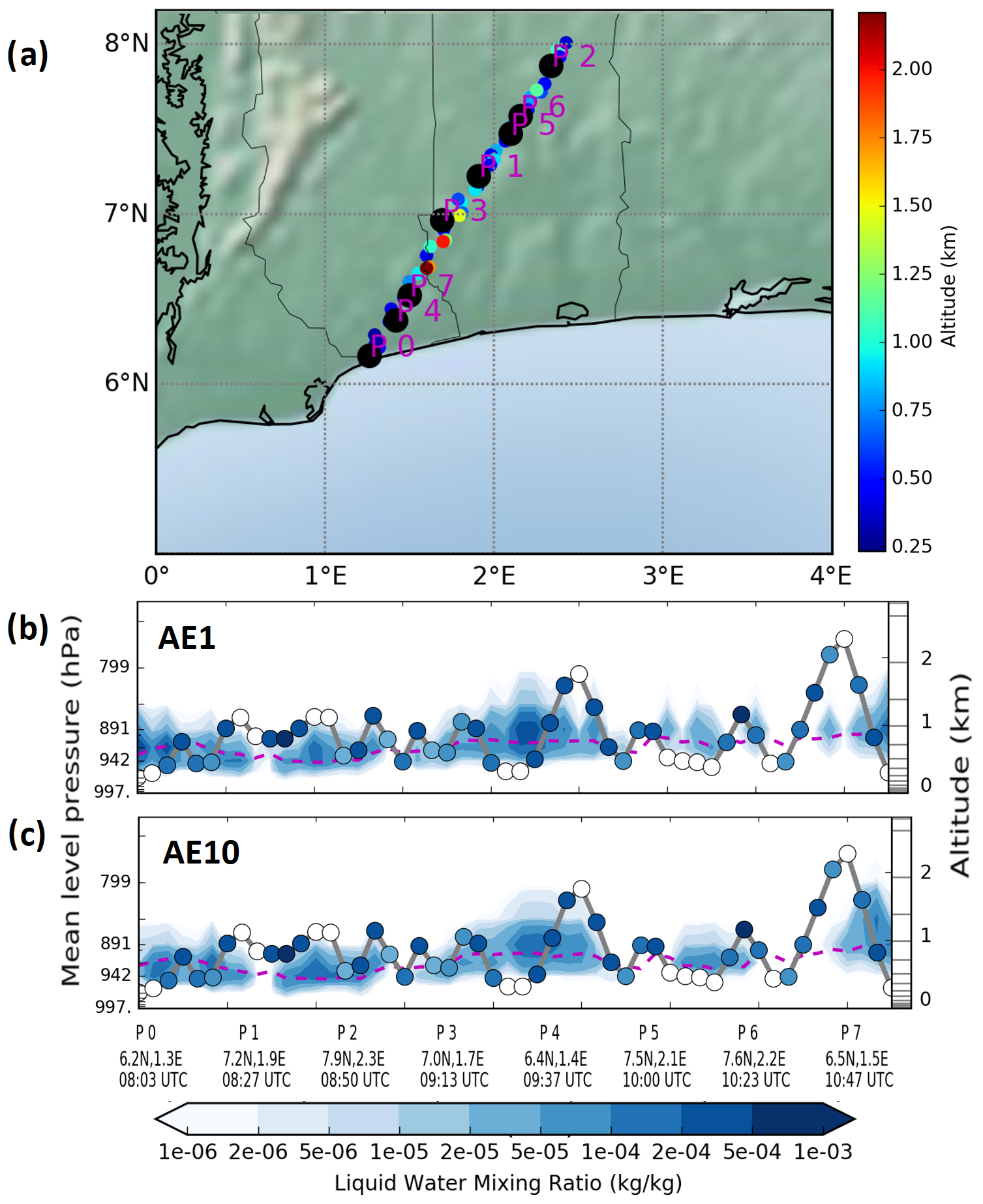
Figure 5Vertical cross section of the liquid water mixing ratio (in kg kg−1) along the trajectory of the ATR-42 research aircraft on 5 July 2016 denoted on the map (a). The 3 min averaged observations are displayed by the colored circles and the modeled vertical distribution along the flight positions by the colored fields for the two experiments: (b) AE1 and (c) AE10, with modeled planetary boundary layer height (dashed violet line).
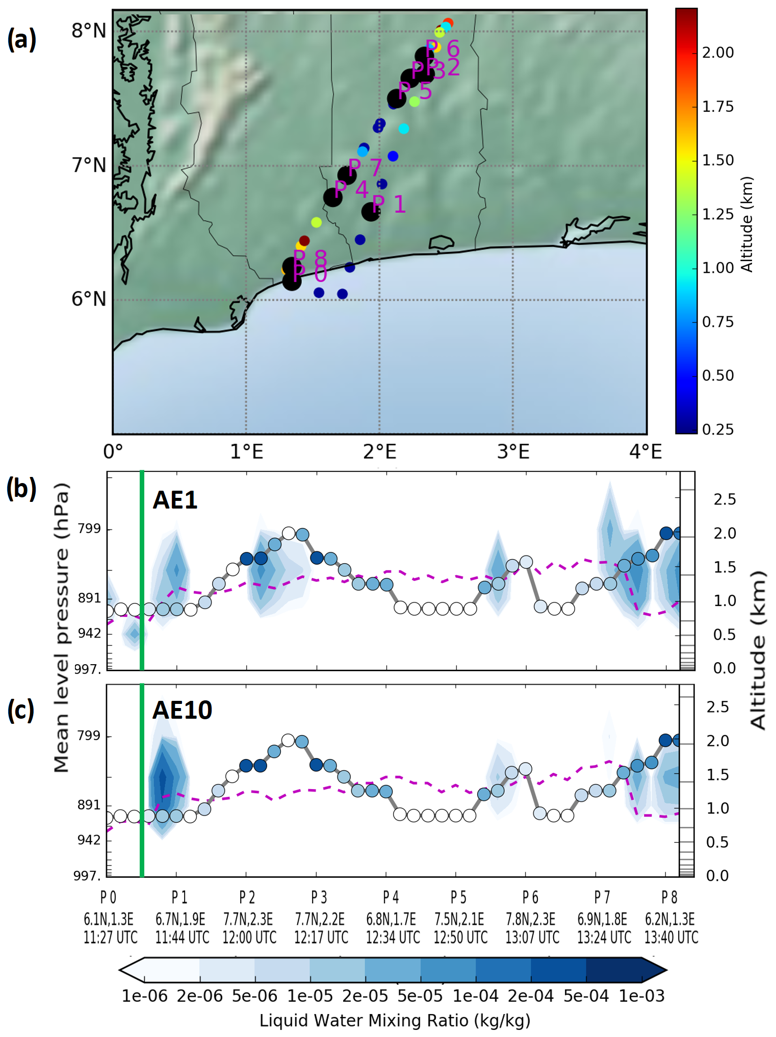
Figure 6Vertical cross section of the liquid water mixing ratio (in kg kg−1) along the trajectory of the Falcon-20 research aircraft on 5 July 2016 denoted on the map (a). The 3 min averaged observations are displayed by the colored circles and the modeled vertical distribution along the flight positions by the colored fields for the two experiments: (b) AE1 and (c) AE10, with modeled planetary boundary layer height (dashed violet line). The green bars indicate the time of the picture taken from the cockpit presented in Fig. A2).
In the morning between Lomé and Savè, the ATR-42 measured a homogenous LLC cover between 0.5 and 2 km a.m.s.l. The LWMR measured in clouds ranges from 10−5 to 10−3 (kg kg−1). LLC are vertically located near the modeled PBL top, ranging between 700 and 1000 m a.m.s.l. The model predicts a similar magnitude of LWMR for AE10 than AE1, which matches with the observations in terms of altitude and magnitude. The modeled LWMR ranges from 10−5 to 5 × 10⁻⁴ (kg kg−1), thus its maximum is underestimated compared to observations. Nevertheless, the spatial variability as well as the altitude of LLC are in good agreement with the observations for both experiments.
At noon, as measured by the Falcon-20 instrumentation (Voigt et al., 2010), the modeled PBL top is higher (ranging between 700 and 1700 m a.m.s.l.) than for the ATR-42 flight and fewer clouds are observed, which is reproduced by the model. The model underestimates the LLC cover, which seems to be lower over the continent for the AE10 experiment. When the Falcon-20 flew over the ocean towards the coast (green bar on Fig. 6 corresponding to the picture of the cockpit from a camera, cf. Fig. A2), a clear front of LLC is facing the aircraft a few hundred meters behind the shore. The aircraft sampled the lower part of the modeled front of LLC (about 5 × 10⁻⁵ kg kg−1) with its cloud instrumentation (Voigt et al., 2011; Kleine et al., 2018). The model reproduces this coastal front, which simulates with the highest LWMR for the AE10 experiment. From 09:00 to 15:00 UTC, there is an accumulation of anthropogenic pollutants at the coast (Deroubaix et al., 2019), which could explain the important difference between the two emission scenarios (AE10 and AE1). In conclusion, the variability of the LWMR is close for the two experiments, and in good agreement with the aircraft measurements.
The spatial analysis of the 5 July flights is completed by a temporal analysis of the LLC altitude over the studied week at the site of Savè. We use the data of cloud base height (CBH) estimated by the ceilometer based on a manufactured software (Handwerker et al., 2016) to compute an hourly average, and we compare it to the modeled vertical distribution of LWMR interpolated at the Savè location for the two experiments (Fig. 7).
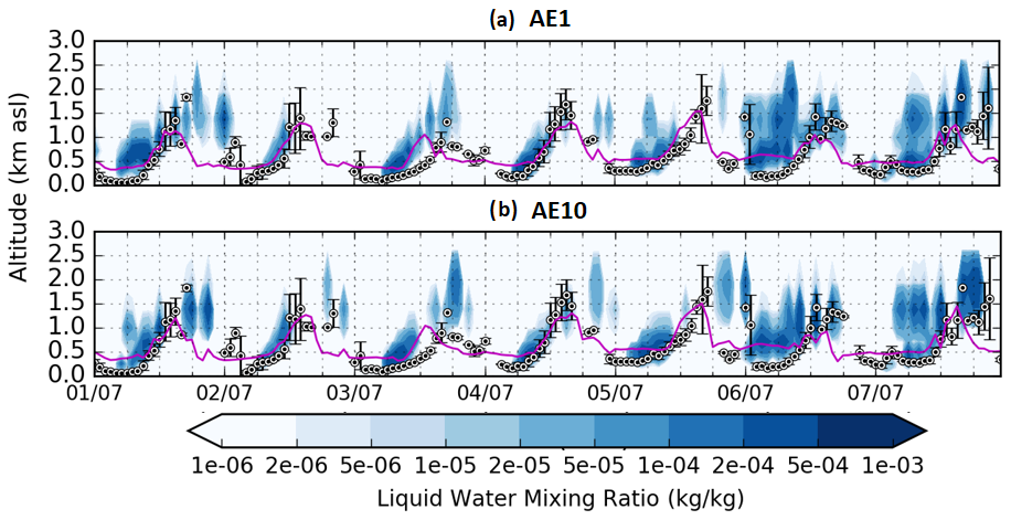
Figure 7Cloud base height at Savè (Benin) measured with the ceilometer (the black circles represent the hourly averages and the bars represent the hourly standard deviation), and compared to the modeled vertical distribution (blueish color shading) of liquid water mixing ratio (kg kg−1) interpolated at Savè in Benin (8.03∘ N, 2.49∘ E) for the two experiments (a) AE1 and (b) AE10, with the modeled planetary boundary layer height (violet line).
In Savè, there is a clear diurnal cycle of LLC because they form at low altitude (few hundred meters) during the night, get elevated by the increase of the PBL height until noon, and break up between 12:00 and 18:00 UTC (Dione et al., 2019; Zouzoua et al., 2021). We note that in the morning, the clouds are always present, mostly with CBH below 500 m a.m.s.l. From 06:00 and 12:00 UTC, the CBH rises up to 1 km a.m.s.l. From 12:00 to 18:00 UTC, the variability (shown by the standard deviation, vertical bars in Fig. 7) of CBH increases, because LLC break up and dissipate around this time (Dione et al., 2019; Zouzoua et al., 2021). From 18:00 to 00:00 UTC, less LLC are observed.
We compare the altitude of the observed hourly CBH evolution to the modeled LWMR vertical patterns in order to analyze the LLC formation, elevation and breakup time. The modeled LWMR for the two experiments reproduces the LLC diurnal cycle depicted above, since we can see the bottom of the modeled clouds, which correspond to LWMR ranging from 10−5 to 5 × 10⁻⁴ kg kg−1, moving vertically from below 500 to 1000 m a.m.s.l. (in blue in Fig. 7). The observed CBH during the morning is in good agreement with the height of the PBL where the modeled cloud base is located. It seems that the duration of the LLC in the afternoon lasts longer in AE10 compared to AE1, and that from 12:00 to 00:00 UTC, the LWMR is slightly higher for the AE10 than AE1.
Both experiments reproduce a realistic temporal variability of LWMR in the studied region. The main differences between the two experiments occur between 12:00 and 00:00 UTC during the LLC breakup time. In the AE10 experiment, LLC lasts longer. However, these differences are small. In order to understand the differences between the two experiments, we need to analyze carefully the modeled features of the LLC diurnal cycle in terms of timing, intensity, and altitude, as well as the implications for precipitation.
In the following, we carry out an analysis of an “Inland” area going from 7∘ N (not including the coastline) to 9∘ N, and from 1 to 4∘ E (Savé is in the middle of this area), which is flat terrain with little elevation without any major city, and thus few anthropogenic emission sources. It is an important region for agriculture (mostly composed of tree crops, cereal, and root vegetables according to the farming system maps produced by the Food and Agriculture Organization of the United Nations), potentially strongly affected by modifications of LLC and precipitation. Using spatial averages of the modeled fields over this area, we analyze the effect of the anthropogenic aerosol load increase on LWMR, liquid water path(LWP), and precipitation rate.
We compute the modeled LWP expressed in mass of water per square meter (kg m−2) in the lowermost troposphere (below 2 km a.m.s.l.) from the LWMR expressed in mass of water divided by mass of air (kg kg−1), using the modeled air density (Mair in kg m−3) and height of the vertical levels (Hlevel in m) with the following formula:
The hourly evolution of the LWMR, LWP, and precipitation are averaged over the “Inland” area (red square on Fig. 1). We analyze each day and the averaged diurnal cycles (with hourly mean and standard deviation) in order to analyze which features are seen every day, and to understand the main differences between AE1 and AE10 (Figs. 8, 9 and 10).
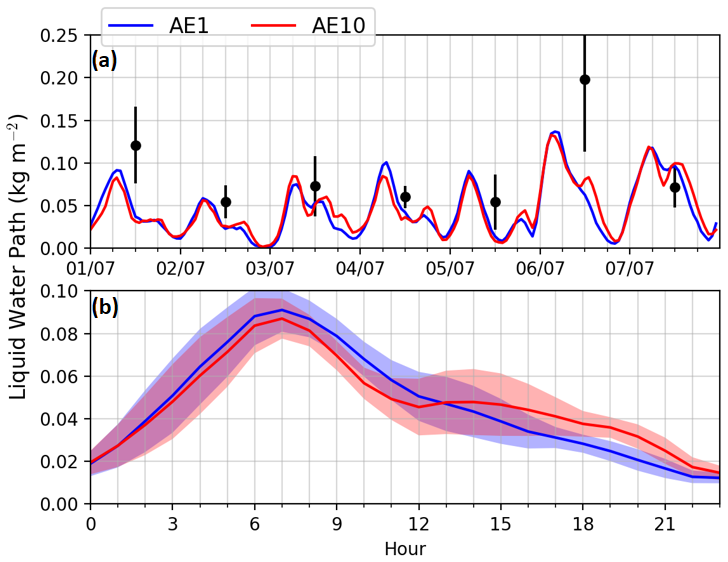
Figure 8Time series (a) and diurnal cycles (b) of modeled hourly liquid water path (kg m−2) for the two experiments, AE1 (blue) and AE10 (red), averaged over an inland area extending from 7 to 9∘ N, and from 1 to 4∘ E, and for the period 1–7 July 2016. (a) The vertical dashed lines indicate periods of 6 h starting at 00:00 UTC. (b) Means of each hour for the period 1–7 July 2016 are presented by lines, and the upper and lower shading limits correspond to the hourly standard deviation. Daily averages of the Moderate Resolution Imaging Spectroradiometer (MODIS) data retrieved by the instruments on the Terra and the Aqua satellites (datasets: MCD06COSP-D3) are black dots with the error bars representing the standard deviation in the area.
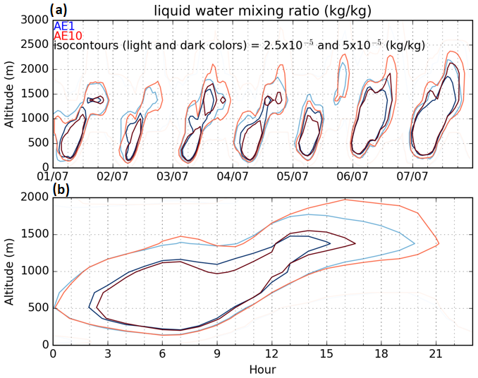
Figure 9Time series of the vertical profile of modeled iso-contours of hourly liquid water mixing ratio (2.5 and 5 × 10⁻⁵ kg kg−1) for the two experiments AE1 (light and dark blue) and AE10 (light and dark red) averaged over an inland area ranging from 7 to 9∘ N, and from 1 to 4∘ E for (a) the period 1–7 July 2016, and (b) means of each hour for this period.
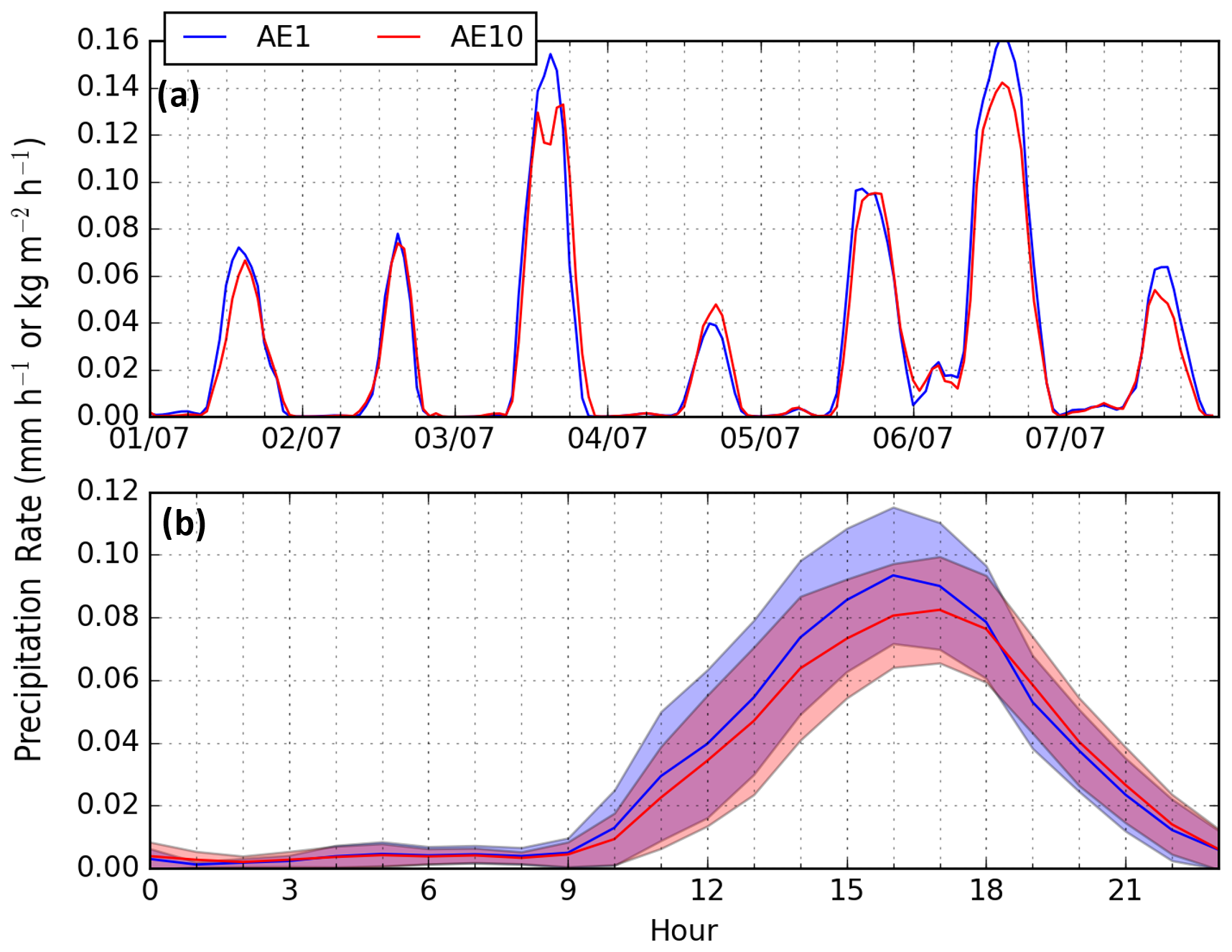
Figure 10Time series (a) and diurnal cycles (b) of modeled hourly precipitation rate (kg m−2) for the two experiments, AE1 (blue) and AE10 (red), averaged over an inland area extending from 7 to 9∘ N, and from 1 to 4∘ E for the period 1–7 July 2016. (a) The vertical dashed lines indicate periods of 6 h starting at 00:00 UTC. (b) Means of each hour for the period 1–7 July 2016 are presented by lines, and the upper and lower shading limits correspond to the hourly standard deviation.
The modeled LWP agrees with the LWP retrieved by MODIS in the sense that, for both, the minimum LWP occurs on 2 July and the maximum LWP occurs on 6 July, although the model is slightly lower than the MODIS estimate (Fig. 8b). The model simulates an increase of the LWP from 00:00 to 07:00 UTC, and a decrease from 07:00 to 00:00 UTC for the two experiments. This diurnal cycle is observed every day (Fig. 8a). We note again that, from 07:00 to 13:00 UTC, the LWP in AE10 is slightly lower than in AE1, then from 13:00 to 22:00 UTC, the LWP in AE10 is higher than in AE1. The LWP in AE1 and AE10 differ mostly from 13:00 to 22:00 UTC (shadings corresponding to mean ± SD are less overlapping in Fig. 8b). In the averaged diurnal cycle (Fig. 8b), the hourly LWP relative change from AE1 to AE10, i.e., (AE10 − AE1) AE1, reaches −16 % at 11:00 UTC, while it is higher than +20 % from 16:00 to 22:00 UTC, even reaching +48 % at 20:00 UTC.
In order to understand how anthropogenic emissions affect the vertical distribution of LWMR, the diurnal evolution is analyzed using two iso-contours relevant for high cloudiness (two iso-contours equal to 2.5 × 10⁻⁵ and to 5 × 10⁻⁵ kg kg−1) in the lowermost troposphere (Fig. 9). We note that for both experiments, (i) the two iso-contours of LWMR appear during the night at the same time for both experiments (at 00:00 and 02:00 UTC, respectively), (ii) the LLC altitude (i.e., low and high parts of the iso-contours) rises from 500 m a.m.s.l. at the beginning of the night to 1400 m at the end of the afternoon, (iii) the main differences between the two simulations occur from 14:00 to 21:00 UTC because the presence of the two iso-contours is delayed by 1 hour for AE10 compared to AE1.
Finally, we analyze the modeled diurnal cycle of precipitation for the two simulations (Fig. 10). The precipitation rates also show a clear cycle every day, occurring from 09:00 to 22:00 UTC in the “Inland” area, which is in agreement with in-situ hourly precipitation measurements (Kalthoff et al., 2018; Knippertz et al., 2017). The more intense hourly precipitation rates are modeled for AE1 with about 0.10 mm occurring at 16:00 UTC, and for AE10 with about 0.08 mm occurring at 17:00 UTC (Fig. 10b). In the averaged diurnal cycle, the relative change in hourly precipitation from AE1 to AE10 reaches −28 % at 16:00 UTC and −23 % at 17:00 UTC. However, the differences concern mostly precipitation rates greater than 0.1 mm h−1 that occurred only on 3 and 6 June 2016 (Fig. 10a).
In our simulations, both the semi-direct and the indirect effects are taken into account, which act simultaneously on evaporation and on precipitation. An increase in the aerosol load may not result in an increase in LWMR, depending on the change in the entrainment in and around clouds due to the evaporation and precipitation of cloud liquid water (e.g., Hill et al., 2009; Toll et al., 2019). The differences between the two experiments (AE10 − AE1) are small for temperature and specific humidity, less than 1 % (with maximum hourly differences reaching 0.24 ∘C and 0.0003 kg kg−1 respectively), and high for liquid water mixing ratio and rain mixing ratio, around −20 % (with maximum hourly differences reaching 10−5 and 10−7 kg kg−1 respectively), which suggests that the reduction in precipitation is mainly related to wetter clouds (Fig. A3). Nevertheless, with our experiments, it is not possible to distinguish the influence of evaporation by the semi-direct effect and of precipitation by the indirect effect on liquid water because we cannot exclude possible opposing effects on temperature and humidity.
In summary, AE1 produces more precipitation and an earlier maximum, while AE10 starts later and produces less precipitation. This might be attributed to the smaller drops, which sustain cloud cover for longer in the afternoon, as shown in our results. Considering daily averages during the studied week (over the “Inland” area), the AE10 experiment simulates LWMR increased by 2.6 % and precipitation rate reduced by 7.5 % compared to AE1. These low relative changes of LWMR hide contrasted periods between the morning and the afternoon. Thus, we conclude that there is a moderate influence of anthropogenic aerosol emission on LLC and precipitation over this area. Nevertheless, these aerosols modify liquid water patterns in the boundary layer, changing precipitation in the north of the “Inland” area, and potentially also over the ocean, as anthropogenic aerosols are eventually transported over the ocean.
The anthropogenic pollution emitted along the coast of the Gulf of Guinea is mostly transported towards the north in the PBL (Deroubaix et al., 2019), modifying the cloud cover, and in turn the precipitation further inland, as shown in the previous subsection. However, there are tropospheric circulations, due to the mid-level return flow of the coastal shallow circulation, transporting polluted air masses towards the ocean, which have been observed with the aircraft measurements and analyzed by Flamant et al. (2018a). This could strongly modify the LLC and precipitation over the ocean, especially because the aerosol concentration is lower than over the continent.
In this section, we extend the analysis of the temporal variability of LLC and precipitation to a larger region. We study three areas (cf. Fig. 1), namely from north to south: Area-9–11N, from 9 to 11∘ N, Area-7–9N, from 7 to 9∘ N (the area studied in Sect. 5), and Area-5–7N, from 5 to 7∘ N, all three extend from 1 to 4∘ E. Note that the Area-5–7N contains a portion of the ocean from 5 to about 6∘ N.
In a first step, we compare the two experiments with TRMM estimates averaged over the three areas at a daily scale (Fig. 11). In a second step, we compare averages of the relative change in LWP and precipitation rate between the two experiments in average for the three areas. In a third step, we analyze the differences between the AE1 and AE10 experiments in terms of LWP and precipitation rate at an hourly time step using time–latitude Hovmoller diagrams (Figs. 12 and 13).
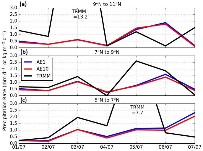
Figure 11Daily precipitation rates measured by the TRMM instrument (black line) and modeled by the AE1 (blue line) and AE10 (red line) experiments for the period 1–7 July 2016, averaged over three areas extending from 1 to 4∘ E, and (a) from 9 to 11∘ N, (b) from 7 to 9∘ N, and (c) from 5 to 7∘ N.
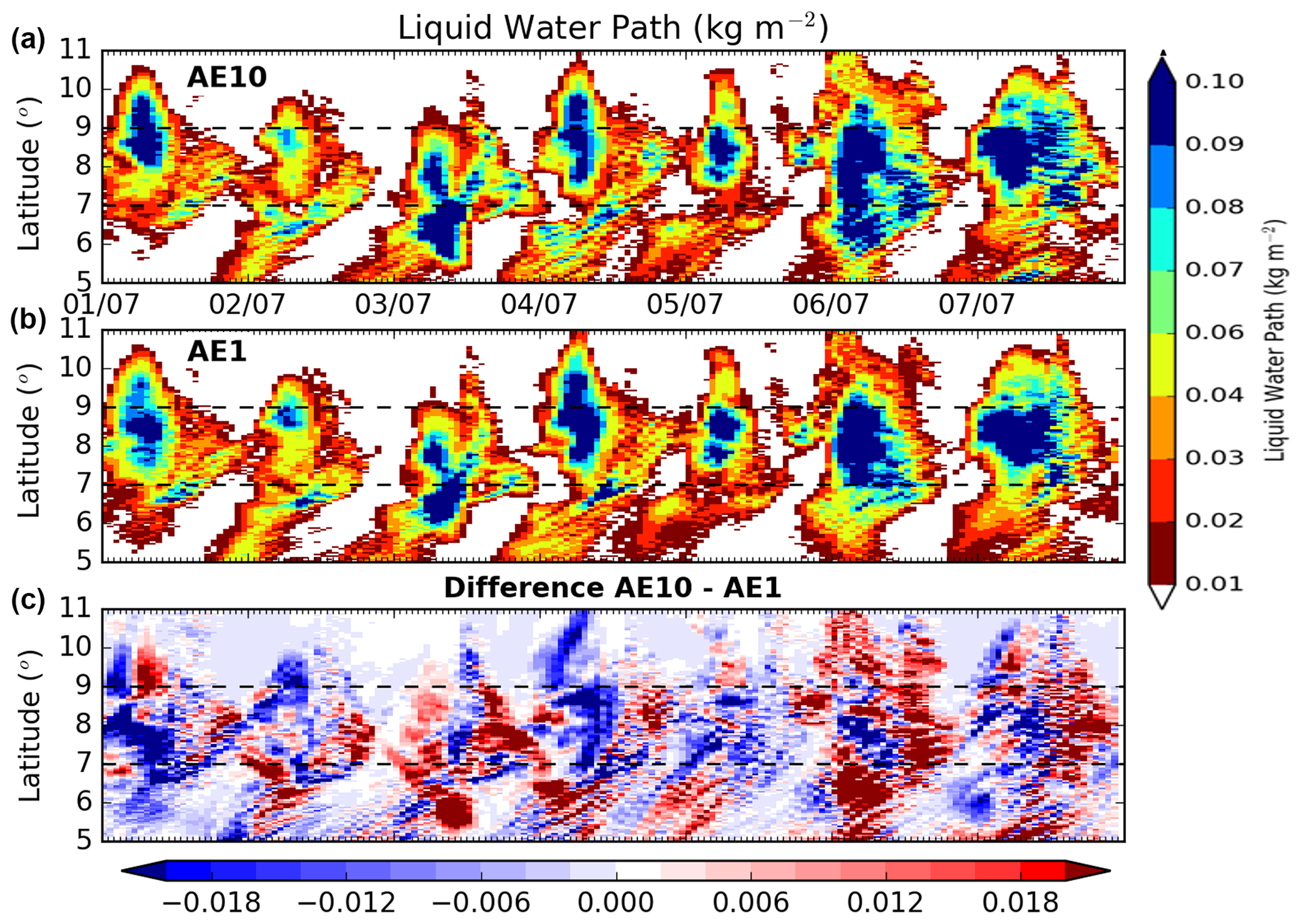
Figure 12Time–latitude average (Hovmoller) of hourly liquid water path (kg m−2) for the two experiments (a) AE10 and (b) AE1, and (c) the difference (AE10 − AE1), averaged over an area extending from 1 to 4∘ E during the period 1–7 July 2016.
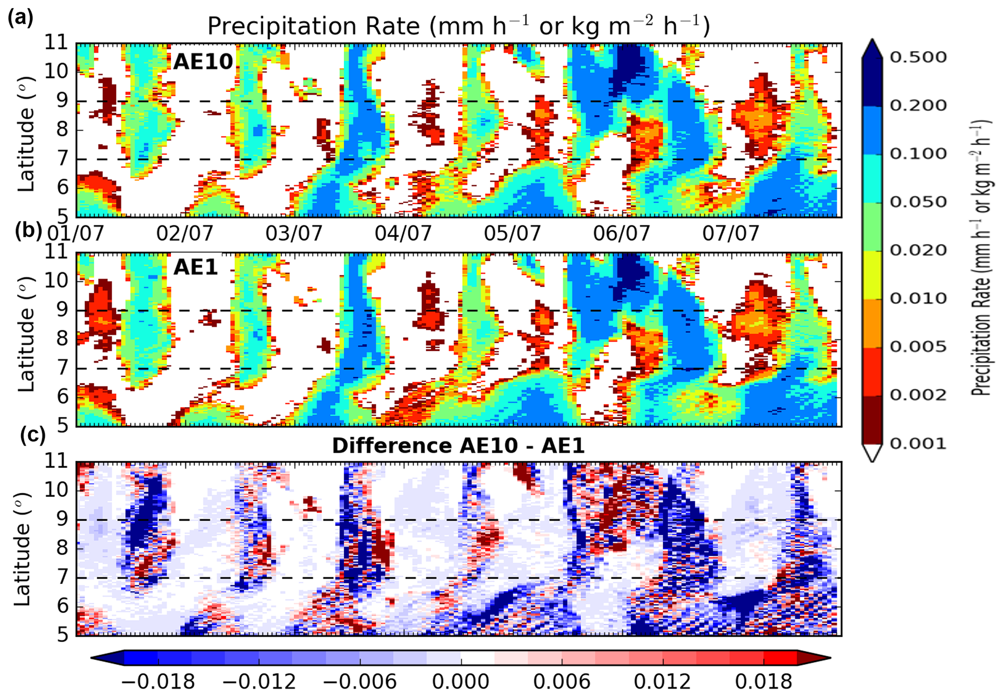
Figure 13Time–latitude average (Hovmoller) of hourly precipitation rate (kg m−2) for the two experiments (a) AE10 and (b) AE1, and (c) the difference (AE10 − AE1) averaged over an area extending from 1 to 4∘ E during the period 1–7 July 2016.
The TRMM estimates show a large day-to-day variability of precipitation rate in the three areas, ranging for Area-9–11N) from 0.1 to 13.2 mm d−1, Area-7–9N) from 0 to 2.5 mm d−1, and Area-5–7N) from 0.2 to 7.7 mm d−1 (Fig. 11). Satellite estimates reveal a larger day-to-day variability than the modeled precipitation rates, which vary from 0.1 to about 2 mm d−1. The maximum modeled precipitation rates are in: Area-9–11N) 1.7 mm d−1 for AE1 and 1.7 mm d−1 for AE10, Area-7–9N) 2.1 mm d−1 for AE1 and 1.8 mm d−1 for AE10, and Area-5–7N) 2.6 mm d−1 for AE1 and 2.0 for AE10. The model reproduces days of light precipitation but days of heavy precipitation are not reproduced.
Even if both state-of-the-art models and satellite products have difficulties in retrieving the precipitation in SWA, this comparison suggests that the model predicts too many days of low precipitation rate, as it has already been shown from comparisons between the observations and the results of the WRF model (Menut et al., 2015, 2019).
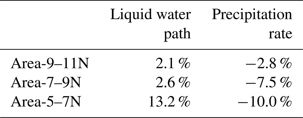
In the area of Savè (Area-7–9N), LWP is increased by 2.6 % in AE10 compared to AE1 on average over the studied week, while the precipitation rate is decreased by −7.5 % (Table 4). North of 9∘ N (Area-9–11N), LWP is increased by 2.1 %, while the precipitation rate is decreased by −2.8 %. The relative difference between the two experiments is greater over the ocean in the Area-5–7N for LWP reaching 13.2 %, and for precipitation rate reaching −10.0 %, which shows the importance of anthropogenic aerosol transported over the ocean where the aerosol load is lower than over the two other areas.
Table 4Relative difference ((AE10 − AE1) AE1) of modeled liquid water path and precipitation rate in average for the three areas: (Area-9–11N) from 9 to 11∘ N, (Area-7–9N) from 7 to 9∘ N, and (Area-5–7N) from 5 to 7∘ N, and extending from 1 to 4∘ E.
To understand the meridional evolution of LWP and precipitation, we investigate the modeled differences with Hovmoller diagrams (time–latitude) from 5 to 11∘ N and averaged over the same longitudes from 1 to 4∘ E. Higher LWP is modeled every day in the Area-7–9N from 03:00 to 09:00 UTC for AE10 and AE1 (Fig. 12), which confirms the homogeneity of the modeled LLC cover over the Savè area.
The modeled spatial variability of the LLC cover is in good agreement with SEVIRI satellite images at 08:00 and 16:00 UTC (Figs. A4 and A6 compared to Figs. A5 and A7). In both experiments, LLC appear first over the ocean in the Area-5–7N at around 18:00 UTC (i.e., LWP > 0.01 kg m−2), and disappear the next day at 12:00 UTC (Fig. 12). We can see a modification along the coastline (about 6∘ N). In the Area-7–9N, this pattern is shifted in time because LLC appear at around 03:00 UTC, and disappear at around 18:00 UTC. In the Area-9–11N, the LLC period is shorter, appearing at 03:00 UTC, and disappearing at 12:00 UTC.
There are contrasting periods of positive/negative difference between AE10 and AE1. In the Area-7–9N, strong positive differences (AE10 − AE1) are observed when cloudiness is high in the afternoon in AE10 (AE10 − AE1 > 0), whereas in the morning, there are mostly negative differences (AE10 − AE1 < 0). Over the ocean (Area-5–7N), there are more LLC in the morning in AE10 (AE10 − AE1 > 0).
Precipitation rates occur in the Area-5–7N over the ocean (from 5 to 6∘ N) every day from midnight to the following morning with slightly higher rates for AE1 compared to AE10 (Fig. 13). We can see that, at the latitude of the coast (between 6 and 6.5∘ N), precipitation rates are decreased in the morning every day. Precipitation rates are highest in the Area-7–9N, occurring during the afternoon over this entire area at the same time.
The high precipitation rates occur at a different time over the ocean between 00:00 and 12:00 UTC, and over the continent between 12:00 and 00:00 UTC. In both simulations, precipitation rates are higher for AE1 compared to AE10. We note that the high precipitation occurring on 6 July during the night in the area-9–11N is stronger for AE10 than AE1 (but precipitation rates that are not in agreement with TRMM measurements on this day).
To conclude, aerosols emitted by anthropogenic activities have a regional scale influence on the LLC and precipitation in our experiments by comparing AE1 to AE10, both inland and over the ocean. The differences for LLC between the two experiments are small on average, however there are contrasting periods during the day.
This study deals with low-level clouds and precipitation over southern West Africa, and focuses on their interactions with anthropogenic aerosols, which are mostly emitted by activities located close to the coast of the Gulf of Guinea. We use the coupled WRF–CHIMERE model making two experiments, which differ solely by the intensity of their anthropogenic emissions. With the HTAP inventory (Janssens-Maenhout et al., 2015) representative of 2010, the experiment underestimates largely the aerosol concentrations in comparison with aircraft measurements during the DACCIWA campaign in July 2016. With the HTAP emissions multiplied by 10, the simulation of the atmospheric aerosol composition is in better agreement with observations of black carbon, organic carbon, ammonium, and nitrate concentrations, which reinforces a major main conclusion of the DACCIWA project, pointing to the importance of using specific anthropogenic emission inventory for southern West Africa (Evans et al., 2018; Keita et al., 2021).
The consideration of different aerosol concentrations in the two experiments does not induce important modifications of humidity and wind speed variability in the lowermost troposphere. The two experiments are realistic and similar for humidity and wind speed. Over an “Inland” area (extending from 7 to 9∘ N and from 1 to 4∘ E), which corresponds to land widely used for agriculture and without any major city, the anthropogenic aerosol increase leads to an increase of hourly low-level cloud cover of more than 20 % in the afternoon, in agreement with Taylor et al. (2019). The breakup time of low-level clouds is delayed by 1 hour, associated with a decrease of precipitation of up to 16 %. The influence of anthropogenic aerosols on low-level clouds is most significant from 16:00 to 21:00 UTC every day, which corresponds to the period of the transport of anthropogenic aerosol from the coastal urbanized area toward the north (Adler et al., 2017; Deetz et al., 2018b; Deroubaix et al., 2019). In contrast, from 09:00 to 15:00 UTC, the anthropogenic aerosols are accumulated along the coastline (Deroubaix et al., 2019), where the modeled low-level cloud cover seems to be sensitive to the anthropogenic aerosol difference between the two experiments.
We conclude that there is a moderate effect of anthropogenic aerosol emissions on low-level clouds and precipitation in SWA from the analysis of our experiments. The long-range transport of aerosol reaching the Gulf of Guinea was significant during the DACCIWA campaign period, mostly because of the biomass burning emission in Central Africa (Haslett et al., 2019; Taylor et al., 2019; Denjean et al., 2020), which is taken into account in the two experiments, contributing to reduce the effect of anthropogenic aerosol emissions. However, our results suggest that local anthropogenic aerosol emissions have an effect on low-level clouds and precipitation over the entire southern West African region, even over the ocean, which highlights the importance of mid-level circulation from the continent to the ocean (Flamant et al., 2018a). The modifications in low-level clouds and precipitation can affect the agricultural activities in this region, and could also have implications for the transition from stratiform to convective clouds (Lohou et al., 2020). Furthermore, the reduction of precipitation in southern West Africa due to the anthropogenic aerosol emitted along the coast, changes the liquid water transported towards the Sahel, and modifies the winds and soil humidity, and as a consequence dust emissions, as shown by Menut et al. (2019). The present study adds evidence to the emerging hypothesis that, during the West African monsoon, increasing anthropogenic aerosol pollution in southern West Africa has already caused a precipitation reduction (Pante et al., 2021).

Figure A1Aerosol Optical Depth (AOD) averaged for the period 1–7 July 2016 for (a) Copernicus Atmosphere Monitoring Service (CAMS) at 09:00 and 13:00 UTC, and for (b) the Moderate Resolution Imaging Spectroradiometer (MODIS) retrieved by the instruments on the Terra and the Aqua satellites (datasets: MOD08-D3 and MID08-D3). Missing values in (b) are colored in gray. The green rectangle represents the studied domain.
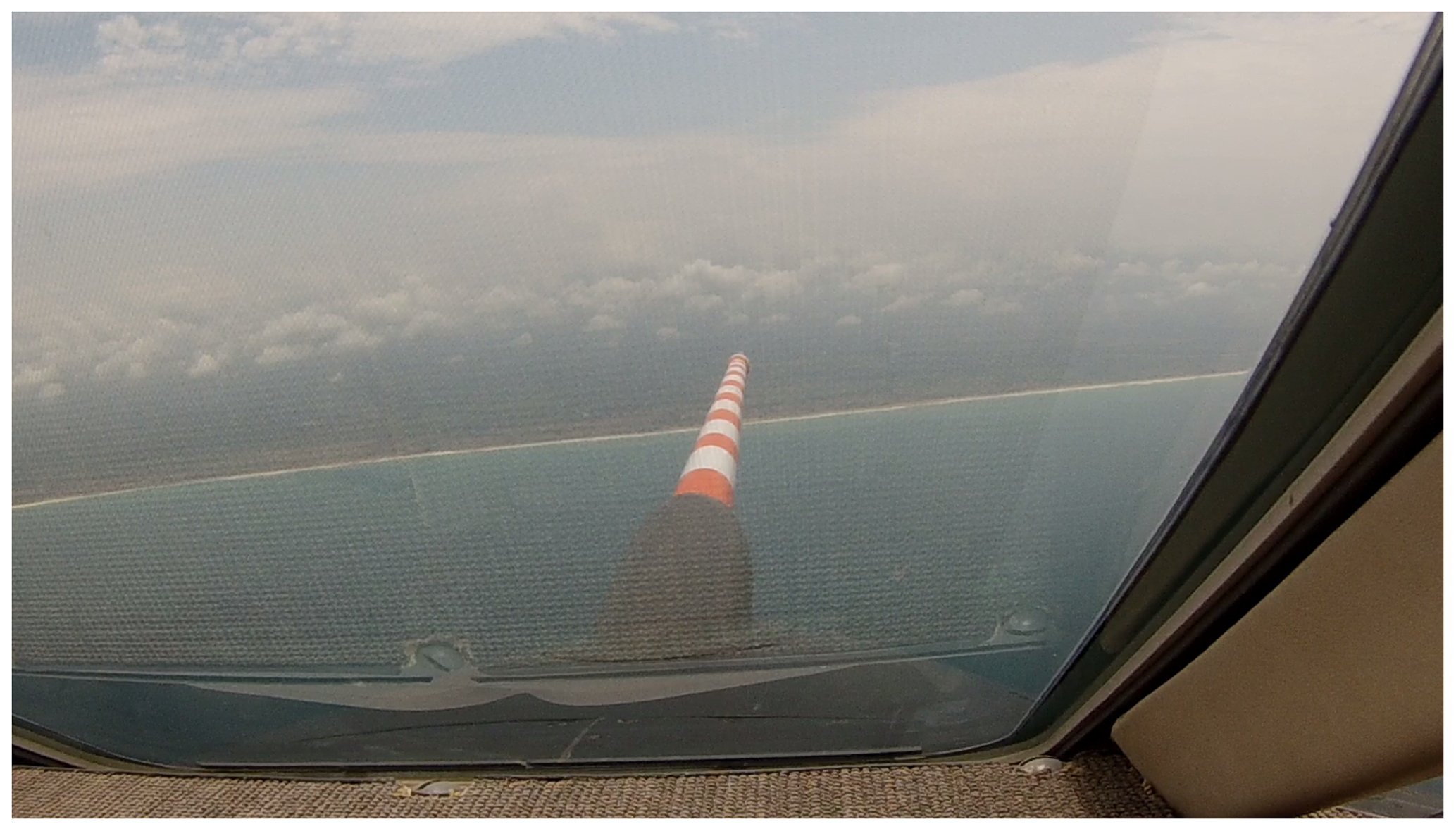
Figure A2Image from the cockpit of the Falcon-20 operated by the DLR for the flight conducted on 5 July 2016 at 11:35 UTC taken in front of the shore of the Gulf of Guinea (at 6.4∘ N, 1.6∘ E, 1 km a.m.s.l.).
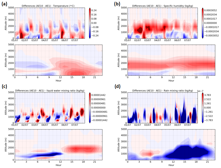
Figure A3Time series of vertical profiles of the differences between the two experiments (AE10 − AE1) for (a) temperature, (b) specific humidity, (c) liquid water mixing ratio, and (d) rain mixing ratio, averaged over an inland area ranging from 7 to 9∘ N, and from 1 to 4∘ E for (a, b) the period 1–7 July 2016, and (c, d) means of each hour for this period.

Figure A4Images by the Spinning Enhanced Visible and Infra-Red Imager (SEVIRI) provided by EuMetSat and NAScube over the studied domain at 08:00 UTC for the period 1–6 July 2016.
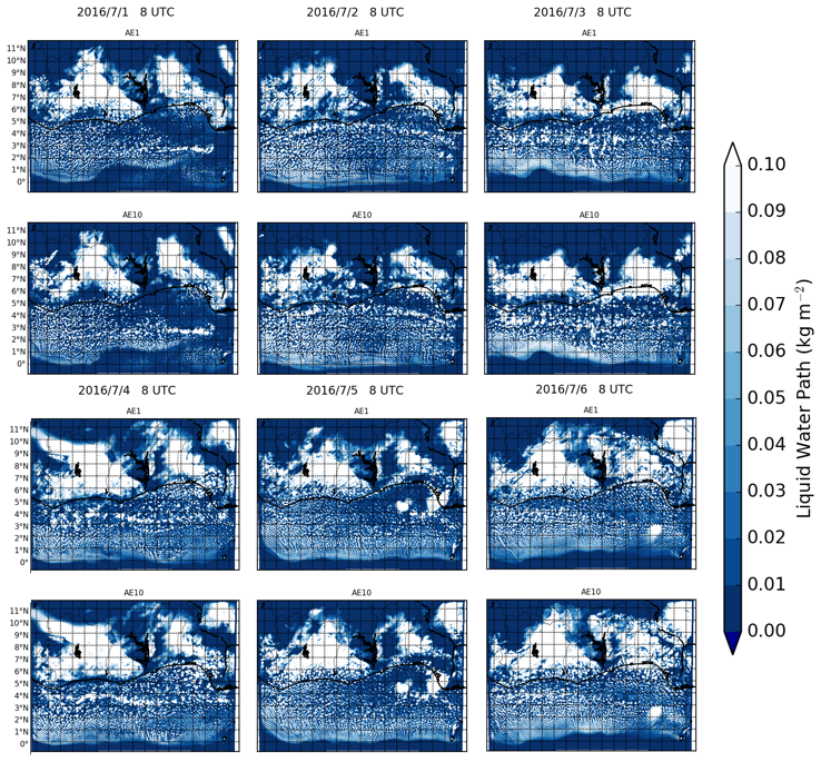
Figure A5Modeled Liquid Water Path over the studied domain at 08:00 UTC for the period 1–6 July 2016.
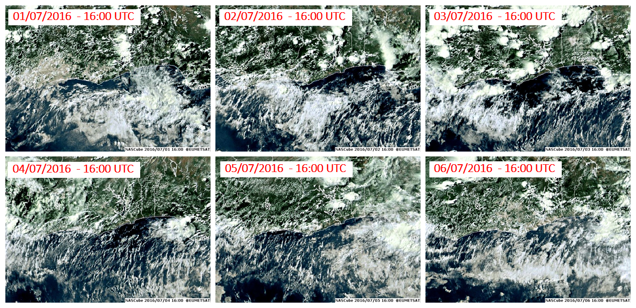
Figure A6Images by the Spinning Enhanced Visible and Infra-Red Imager (SEVIRI) provided by EuMetSat and NAScube over the studied domain at 16:00 UTC for the period 1–6 July 2016.
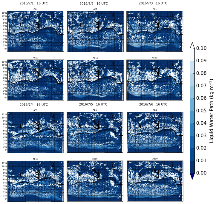
Figure A7Modeled Liquid Water Path over the studied domain at 16:00 UTC for the period 1–6 July 2016.
The aircraft measurements taken during the DACCIWA field campaign can be obtained from https://baobab.sedoo.fr/ (last access: 7 March 2022) after (free) registration or https://doi.org/10.6096/dacciwa.1618 (Derrien and Bezombes, 2016).
AD designed the study, performed the data analysis and produced the figures. AD, CF and LM wrote the initial version of the paper. All co-authors contributed to the interpretation of the results and edited the final version of the paper.
The contact author has declared that neither they nor their co-authors have any competing interests.
Publisher’s note: Copernicus Publications remains neutral with regard to jurisdictional claims in published maps and institutional affiliations.
The Service des Avions Français Instrumentés pour la Recherche en Environnement (SAFIRE, a joint entity of CNRS, Météo-France and CNES and operator of the ATR-42), the British Antarctic Survey (BAS, operator of the Twin Otter) and the Deutsches Zentrum für Luft und Raumfahrt (operator of the Falcon-20) are thanked for their support. We acknowledge the AMS team of the Falcon-20, Stephan Borrmann, Johannes Schneider and Christiane Schulz, for providing data. Christiane Voigt acknowledges funding within the DFG SPP PROM by contract number VO 1504/5-1.
The research leading to these results has been supported by the European Union 7th Framework Programme (FP7/2007-2013) under Grant Agreement no. 603502 (EU project DACCIWA: Dynamics-aerosol-chemistry-cloud interactions in West Africa).
This paper was edited by Nikos Hatzianastassiou and reviewed by four anonymous referees.
Abdul-Razzak, H.: A parameterization of aerosol activation 3. Sectional representation, J. Geophys. Res., 107, 4026, https://doi.org/10.1029/2001JD000483, 2002. a, b
Adler, B., Kalthoff, N., and Gantner, L.: Nocturnal low-level clouds over southern West Africa analysed using high-resolution simulations, Atmos. Chem. Phys., 17, 899–910, https://doi.org/10.5194/acp-17-899-2017, 2017. a, b
Adler, B., Babić, K., Kalthoff, N., Lohou, F., Lothon, M., Dione, C., Pedruzo-Bagazgoitia, X., and Andersen, H.: Nocturnal low-level clouds in the atmospheric boundary layer over southern West Africa: an observation-based analysis of conditions and processes, Atmos. Chem. Phys., 19, 663–681, https://doi.org/10.5194/acp-19-663-2019, 2019. a, b
Ayers, G.: Comment on regression analysis of air quality data, Atmos. Environ., 35, 2423–2425, https://doi.org/10.1016/S1352-2310(00)00527-6, 2001. a
Babić, K., Adler, B., Kalthoff, N., Andersen, H., Dione, C., Lohou, F., Lothon, M., and Pedruzo-Bagazgoitia, X.: The observed diurnal cycle of low-level stratus clouds over southern West Africa: a case study, Atmos. Chem. Phys., 19, 1281–1299, https://doi.org/10.5194/acp-19-1281-2019, 2019. a
Baklanov, A., Schlünzen, K., Suppan, P., Baldasano, J., Brunner, D., Aksoyoglu, S., Carmichael, G., Douros, J., Flemming, J., Forkel, R., Galmarini, S., Gauss, M., Grell, G., Hirtl, M., Joffre, S., Jorba, O., Kaas, E., Kaasik, M., Kallos, G., Kong, X., Korsholm, U., Kurganskiy, A., Kushta, J., Lohmann, U., Mahura, A., Manders-Groot, A., Maurizi, A., Moussiopoulos, N., Rao, S. T., Savage, N., Seigneur, C., Sokhi, R. S., Solazzo, E., Solomos, S., Sørensen, B., Tsegas, G., Vignati, E., Vogel, B., and Zhang, Y.: Online coupled regional meteorology chemistry models in Europe: current status and prospects, Atmos. Chem. Phys., 14, 317–398, https://doi.org/10.5194/acp-14-317-2014, 2014. a
Baklanov, A., Brunner, D., Carmichael, G., Flemming, J., Freitas, S., Gauss, M., Hov, O., Mathur, R., Schlünzen, K. H., Seigneur, C., and Vogel, B.: Key Issues for Seamless Integrated Chemistry–Meteorology Modeling, B. Am. Meteorol. Soc., 98, 2285–2292, https://doi.org/10.1175/BAMS-D-15-00166.1, 2017. a
Bauer, S. E., Im, U., Mezuman, K., and Gao, C. Y.: Desert Dust, Industrialization, and Agricultural Fires: Health Impacts of Outdoor Air Pollution in Africa, J. Geophys. Res.-Atmos., 124, 4104–4120, https://doi.org/10.1029/2018JD029336, 2019. a
Berry, E. X. and Reinhardt, R. L.: An Analysis of Cloud Drop Growth by Collection Part II. Single Initial Distributions, J. Atmos. Sci., 31, 1825–1831, https://doi.org/10.1175/1520-0469(1974)031<1825:AAOCDG>2.0.CO;2, 1974. a
Bessagnet, B., Hodzic, a., Vautard, R., Beekmann, M., Cheinet, S., Honoré, C., Liousse, C., and Rouil, L.: Aerosol modeling with CHIMERE – Preliminary evaluation at the continental scale, Atmos. Environ., 38, 2803–2817, https://doi.org/10.1016/j.atmosenv.2004.02.034, 2004. a
Briant, R., Tuccella, P., Deroubaix, A., Khvorostyanov, D., Menut, L., Mailler, S., and Turquety, S.: Aerosol–radiation interaction modelling using online coupling between the WRF 3.7.1 meteorological model and the CHIMERE 2016 chemistry-transport model, through the OASIS3-MCT coupler, Geosci. Model Dev., 10, 927–944, https://doi.org/10.5194/gmd-10-927-2017, 2017. a, b
Brito, J., Freney, E., Dominutti, P., Borbon, A., Haslett, S. L., Batenburg, A. M., Colomb, A., Dupuy, R., Denjean, C., Burnet, F., Bourriane, T., Deroubaix, A., Sellegri, K., Borrmann, S., Coe, H., Flamant, C., Knippertz, P., and Schwarzenboeck, A.: Assessing the role of anthropogenic and biogenic sources on PM1 over southern West Africa using aircraft measurements, Atmos. Chem. Phys., 18, 757–772, https://doi.org/10.5194/acp-18-757-2018, 2018. a, b
Carslaw, K. S., Boucher, O., Spracklen, D. V., Mann, G. W., Rae, J. G. L., Woodward, S., and Kulmala, M.: A review of natural aerosol interactions and feedbacks within the Earth system, Atmos. Chem. Phys., 10, 1701–1737, https://doi.org/10.5194/acp-10-1701-2010, 2010. a, b
Chapman, E. G., Gustafson Jr., W. I., Easter, R. C., Barnard, J. C., Ghan, S. J., Pekour, M. S., and Fast, J. D.: Coupling aerosol-cloud-radiative processes in the WRF-Chem model: Investigating the radiative impact of elevated point sources, Atmos. Chem. Phys., 9, 945–964, https://doi.org/10.5194/acp-9-945-2009, 2009. a
Craig, A., Valcke, S., and Coquart, L.: Development and performance of a new version of the OASIS coupler, OASIS3-MCT_3.0, Geosci. Model Dev., 10, 3297–3308, https://doi.org/10.5194/gmd-10-3297-2017, 2017. a
Deetz, K., Vogel, H., Haslett, S., Knippertz, P., Coe, H., and Vogel, B.: Aerosol liquid water content in the moist southern West African monsoon layer and its radiative impact, Atmos. Chem. Phys., 18, 14271–14295, https://doi.org/10.5194/acp-18-14271-2018, 2018a. a
Deetz, K., Vogel, H., Knippertz, P., Adler, B., Taylor, J., Coe, H., Bower, K., Haslett, S., Flynn, M., Dorsey, J., Crawford, I., Kottmeier, C., and Vogel, B.: Numerical simulations of aerosol radiative effects and their impact on clouds and atmospheric dynamics over southern West Africa, Atmos. Chem. Phys., 18, 9767–9788, https://doi.org/10.5194/acp-18-9767-2018, 2018b. a, b
Denjean, C., Bourrianne, T., Burnet, F., Mallet, M., Maury, N., Colomb, A., Dominutti, P., Brito, J., Dupuy, R., Sellegri, K., Schwarzenboeck, A., Flamant, C., and Knippertz, P.: Overview of aerosol optical properties over southern West Africa from DACCIWA aircraft measurements, Atmos. Chem. Phys., 20, 4735–4756, https://doi.org/10.5194/acp-20-4735-2020, 2020. a, b
Derrien, S. and Bezombes, Y.: DACCIWA field campaign, Savè super-site, UPS instrumentation, SEDOO OMP [data set], https://doi.org/10.6096/dacciwa.1618, 2016. a
Deroubaix, A., Flamant, C., Menut, L., Siour, G., Mailler, S., Turquety, S., Briant, R., Khvorostyanov, D., and Crumeyrolle, S.: Interactions of atmospheric gases and aerosols with the monsoon dynamics over the Sudano-Guinean region during AMMA, Atmos. Chem. Phys., 18, 445–465, https://doi.org/10.5194/acp-18-445-2018, 2018. a, b
Deroubaix, A., Menut, L., Flamant, C., Brito, J., Denjean, C., Dreiling, V., Fink, A., Jambert, C., Kalthoff, N., Knippertz, P., Ladkin, R., Mailler, S., Maranan, M., Pacifico, F., Piguet, B., Siour, G., and Turquety, S.: Diurnal cycle of coastal anthropogenic pollutant transport over southern West Africa during the DACCIWA campaign, Atmos. Chem. Phys., 19, 473–497, https://doi.org/10.5194/acp-19-473-2019, 2019. a, b, c, d, e, f, g, h, i
Dione, C., Lohou, F., Lothon, M., Adler, B., Babić, K., Kalthoff, N., Pedruzo-Bagazgoitia, X., Bezombes, Y., and Gabella, O.: Low-level stratiform clouds and dynamical features observed within the southern West African monsoon, Atmos. Chem. Phys., 19, 8979–8997, https://doi.org/10.5194/acp-19-8979-2019, 2019. a, b, c, d
Ek, M. B., Mitchell, K. E., Lin, Y., Rogers, E., Grunmann, P., Koren, V., Gayno, G., and Tarpley, J. D.: Implementation of Noah land surface model advances in the National Centers for Environmental Prediction operational mesoscale Eta model, J. Geophys. Res.-Atmos., 108, 8851, https://doi.org/10.1029/2002JD003296, 2003. a
Evans, M., Knippertz, P., Akpo, A., Allan, R. P., Amekudzi, L., Brooks, B., Chiu, J. C., Coe, H., Fink, A. H., Flamant, C., Jegede, O. O., Leal-Liousse, C., Lohou, F., Kalthoff, N., Mari, C., Marsham, J. H., Yoboué, V., and Zumsprekel, C. R.: Policy findings from the DACCIWA Project (Version 1), Zenodo, https://doi.org/10.5281/zenodo.1476843, 2018. a
Fan, J., Wang, Y., Rosenfeld, D., and Liu, X.: Review of Aerosol–Cloud Interactions: Mechanisms, Significance, and Challenges, J. Atmos. Sci., 73, 4221–4252, https://doi.org/10.1175/JAS-D-16-0037.1, 2016. a
Flamant, C., Deroubaix, A., Chazette, P., Brito, J., Gaetani, M., Knippertz, P., Fink, A. H., de Coetlogon, G., Menut, L., Colomb, A., Denjean, C., Meynadier, R., Rosenberg, P., Dupuy, R., Dominutti, P., Duplissy, J., Bourrianne, T., Schwarzenboeck, A., Ramonet, M., and Totems, J.: Aerosol distribution in the northern Gulf of Guinea: local anthropogenic sources, long-range transport, and the role of coastal shallow circulations, Atmos. Chem. Phys., 18, 12363–12389, https://doi.org/10.5194/acp-18-12363-2018, 2018a. a, b, c
Flamant, C., Knippertz, P., Fink, A. H., Akpo, A., Brooks, B., Chiu, C. J., Coe, H., Danuor, S., Evans, M., Jegede, O., Kalthoff, N., Konaré, A., Liousse, C., Lohou, F., Mari, C., Schlager, H., Schwarzenboeck, A., Adler, B., Amekudzi, L., Aryee, J., Ayoola, M., Batenburg, A. M., Bessardon, G., Borrmann, S., Brito, J., Bower, K., Burnet, F., Catoire, V., Colomb, A., Denjean, C., Fosu-Amankwah, K., Hill, P. G., Lee, J., Lothon, M., Maranan, M., Marsham, J., Meynadier, R., Ngamini, J.-B., Rosenberg, P., Sauer, D., Smith, V., Stratmann, G., Taylor, J. W., Voigt, C., and Yoboué, V.: The Dynamics-Aerosol-Chemistry-Cloud Interactions in West Africa field campaign: Overview and research highlights, B. Am. Meteorol. Soc., 99, 83–104, https://doi.org/10.1175/BAMS-D-16-0256.1, 2018b. a, b
Flatau, P. J., Walko, R. L., and Cotton, W. R.: Polynomial Fits to Saturation Vapor Pressure, J. Appl. Meteorol., 31, 1507–1513, https://doi.org/10.1175/1520-0450(1992)031<1507:PFTSVP>2.0.CO;2, 1992. a
Ghan, S. J., Leung, L. R., Easter, R. C., and Abdul-Razzak, H.: Prediction of cloud droplet number in a general circulation model, J. Geophys. Res.-Atmos., 102, 21777–21794, https://doi.org/10.1029/97JD01810, 1997. a
Grell, G. A. and Freitas, S. R.: A scale and aerosol aware stochastic convective parameterization for weather and air quality modeling, Atmos. Chem. Phys., 14, 5233–5250, https://doi.org/10.5194/acp-14-5233-2014, 2014. a
Handwerker, J., Scheer, S., and Gamer, T.: DACCIWA field campaign, Savé super-site, KIT instrumentation: Cloud and precipitation; SEDOO OMP, https://doi.org/10.6096/DACCIWA.1686, 2016. a
Hannak, L., Knippertz, P., Fink, A. H., Kniffka, A., and Pante, G.: Why Do Global Climate Models Struggle to Represent Low-Level Clouds in the West African Summer Monsoon?, J. Climate, 30, 1665–1687, https://doi.org/10.1175/JCLI-D-16-0451.1, 2017. a
Haslett, S. L., Taylor, J. W., Evans, M., Morris, E., Vogel, B., Dajuma, A., Brito, J., Batenburg, A. M., Borrmann, S., Schneider, J., Schulz, C., Denjean, C., Bourrianne, T., Knippertz, P., Dupuy, R., Schwarzenböck, A., Sauer, D., Flamant, C., Dorsey, J., Crawford, I., and Coe, H.: Remote biomass burning dominates southern West African air pollution during the monsoon, Atmos. Chem. Phys., 19, 15217–15234, https://doi.org/10.5194/acp-19-15217-2019, 2019. a, b, c
Haywood, J. and Boucher, O.: Estimates of the direct and indirect radiative forcing due to tropospheric aerosols: A review, Rev. Geophys., 38, 513–543, https://doi.org/10.1029/1999RG000078, 2000. a
Hill, A. A., Feingold, G., and Jiang, H.: The Influence of Entrainment and Mixing Assumption on Aerosol–Cloud Interactions in Marine Stratocumulus, J. Atmos. Sci., 66, 1450–1464, https://doi.org/10.1175/2008JAS2909.1, 2009. a
Hong, S.-Y., Noh, Y., and Dudhia, J.: A new vertical diffusion package with an explicit treatment of entrainment processes, Mon. Weather Rev., 134, 2318–2341, https://doi.org/10.1175/MWR3199.1, 2006. a
Iacono, M. J., Delamere, J. S., Mlawer, E. J., Shephard, M. W., Clough, S. A., and Collins, W. D.: Radiative forcing by long-lived greenhouse gases: Calculations with the AER radiative transfer models, J. Geophys. Res., 113, D13103, https://doi.org/10.1029/2008JD009944, 2008. a
Inness, A., Ades, M., Agustí-Panareda, A., Barré, J., Benedictow, A., Blechschmidt, A.-M., Dominguez, J. J., Engelen, R., Eskes, H., Flemming, J., Huijnen, V., Jones, L., Kipling, Z., Massart, S., Parrington, M., Peuch, V.-H., Razinger, M., Remy, S., Schulz, M., and Suttie, M.: The CAMS reanalysis of atmospheric composition, Atmos. Chem. Phys., 19, 3515–3556, https://doi.org/10.5194/acp-19-3515-2019, 2019. a
Janjic, Z. I.: The Weather Research and Forecasting Model: Overview, System Efforts, and Future Directions, Meteorol. Atmos. Phys., 82, 1436–5065, https://doi.org/10.1007/s00703-001-0587-6, 2003. a
Janssens-Maenhout, G., Crippa, M., Guizzardi, D., Dentener, F., Muntean, M., Pouliot, G., Keating, T., Zhang, Q., Kurokawa, J., Wankmüller, R., Denier van der Gon, H., Kuenen, J. J. P., Klimont, Z., Frost, G., Darras, S., Koffi, B., and Li, M.: HTAP_v2.2: a mosaic of regional and global emission grid maps for 2008 and 2010 to study hemispheric transport of air pollution, Atmos. Chem. Phys., 15, 11411–11432, https://doi.org/10.5194/acp-15-11411-2015, 2015. a, b
Kalthoff, N., Lohou, F., Brooks, B., Jegede, G., Adler, B., Babić, K., Dione, C., Ajao, A., Amekudzi, L. K., Aryee, J. N. A., Ayoola, M., Bessardon, G., Danuor, S. K., Handwerker, J., Kohler, M., Lothon, M., Pedruzo-Bagazgoitia, X., Smith, V., Sunmonu, L., Wieser, A., Fink, A. H., and Knippertz, P.: An overview of the diurnal cycle of the atmospheric boundary layer during the West African monsoon season: results from the 2016 observational campaign, Atmos. Chem. Phys., 18, 2913–2928, https://doi.org/10.5194/acp-18-2913-2018, 2018. a, b, c, d
Keita, S., Liousse, C., Yoboué, V., Dominutti, P., Guinot, B., Assamoi, E.-M., Borbon, A., Haslett, S. L., Bouvier, L., Colomb, A., Coe, H., Akpo, A., Adon, J., Bahino, J., Doumbia, M., Djossou, J., Galy-Lacaux, C., Gardrat, E., Gnamien, S., Léon, J. F., Ossohou, M., N'Datchoh, E. T., and Roblou, L.: Particle and VOC emission factor measurements for anthropogenic sources in West Africa, Atmos. Chem. Phys., 18, 7691–7708, https://doi.org/10.5194/acp-18-7691-2018, 2018. a
Keita, S., Liousse, C., Assamoi, E.-M., Doumbia, T., N'Datchoh, E. T., Gnamien, S., Elguindi, N., Granier, C., and Yoboué, V.: African anthropogenic emissions inventory for gases and particles from 1990 to 2015, Earth Syst. Sci. Data, 13, 3691–3705, https://doi.org/10.5194/essd-13-3691-2021, 2021. a
Kleine, J., Voigt, C., Sauer, D., Schlager, H., Scheibe, M., Jurkat-Witschas, T., Kaufmann, S., Kärcher, B., and Anderson, B. E.: In Situ Observations of Ice Particle Losses in a Young Persistent Contrail, Geophys. Res. Lett., 45, 13553–13561, https://doi.org/10.1029/2018GL079390, 2018. a
Knippertz, P., Coe, H., Chiu, J. C., Evans, M. J., Fink, A. H., Kalthoff, N., Liousse, C., Mari, C., Allan, R. P., Brooks, B., Danour, S., Flamant, C., Jegede, O. O., Lohou, F., and Marsham, J. H.: The DACCIWA project: Dynamics-aerosol-chemistry-cloud interactions in West Africa, B. Am. Meteorol. Soc., 96, 1451–1460, https://doi.org/10.1175/BAMS-D-14-00108.1, 2015a. a
Knippertz, P., Evans, M. J., Field, P. R., Fink, A. H., Liousse, C., and Marsham, J. H.: The possible role of local air pollution in climate change in West Africa, Nat. Clim. Change, 5, 815–822, https://doi.org/10.1038/nclimate2727, 2015b. a
Knippertz, P., Fink, A. H., Deroubaix, A., Morris, E., Tocquer, F., Evans, M. J., Flamant, C., Gaetani, M., Lavaysse, C., Mari, C., Marsham, J. H., Meynadier, R., Affo-Dogo, A., Bahaga, T., Brosse, F., Deetz, K., Guebsi, R., Latifou, I., Maranan, M., Rosenberg, P. D., and Schlueter, A.: A meteorological and chemical overview of the DACCIWA field campaign in West Africa in June–July 2016, Atmos. Chem. Phys., 17, 10893–10918, https://doi.org/10.5194/acp-17-10893-2017, 2017. a, b, c
Liousse, C., Assamoi, E., Criqui, P., Granier, C., and Rosset, R.: Explosive growth in African combustion emissions from 2005 to 2030, Environ. Res. Lett., 9, 035003, https://doi.org/10.1088/1748-9326/9/3/035003, 2014. a, b
Lohou, F., Kalthoff, N., Adler, B., Babić, K., Dione, C., Lothon, M., Pedruzo-Bagazgoitia, X., and Zouzoua, M.: Conceptual model of diurnal cycle of low-level stratiform clouds over southern West Africa, Atmos. Chem. Phys., 20, 2263–2275, https://doi.org/10.5194/acp-20-2263-2020, 2020. a, b, c, d
Mailler, S., Menut, L., Khvorostyanov, D., Valari, M., Couvidat, F., Siour, G., Turquety, S., Briant, R., Tuccella, P., Bessagnet, B., Colette, A., Létinois, L., Markakis, K., and Meleux, F.: CHIMERE-2017: from urban to hemispheric chemistry-transport modeling, Geosci. Model Dev., 10, 2397–2423, https://doi.org/10.5194/gmd-10-2397-2017, 2017. a
Menut, L., Bessagnet, B., Khvorostyanov, D., Beekmann, M., Blond, N., Colette, A., Coll, I., Curci, G., Foret, G., Hodzic, A., Mailler, S., Meleux, F., Monge, J.-L., Pison, I., Siour, G., Turquety, S., Valari, M., Vautard, R., and Vivanco, M. G.: CHIMERE 2013: a model for regional atmospheric composition modelling, Geosci. Model Dev., 6, 981–1028, https://doi.org/10.5194/gmd-6-981-2013, 2013. a
Menut, L., Mailler, S., Siour, G., Bessagnet, B., Turquety, S., Rea, G., Briant, R., Mallet, M., Sciare, J., Formenti, P., and Meleux, F.: Ozone and aerosol tropospheric concentrations variability analyzed using the ADRIMED measurements and the WRF and CHIMERE models, Atmos. Chem. Phys., 15, 6159–6182, https://doi.org/10.5194/acp-15-6159-2015, 2015. a
Menut, L., Siour, G., Mailler, S., Couvidat, F., and Bessagnet, B.: Observations and regional modeling of aerosol optical properties, speciation and size distribution over Northern Africa and western Europe, Atmos. Chem. Phys., 16, 12961–12982, https://doi.org/10.5194/acp-16-12961-2016, 2016. a
Menut, L., Flamant, C., Turquety, S., Deroubaix, A., Chazette, P., and Meynadier, R.: Impact of biomass burning on pollutant surface concentrations in megacities of the Gulf of Guinea, Atmos. Chem. Phys., 18, 2687–2707, https://doi.org/10.5194/acp-18-2687-2018, 2018. a
Menut, L., Tuccella, P., Flamant, C., Deroubaix, A., and Gaetani, M.: The role of aerosol–radiation–cloud interactions in linking anthropogenic pollution over southern west Africa and dust emission over the Sahara, Atmos. Chem. Phys., 19, 14657–14676, https://doi.org/10.5194/acp-19-14657-2019, 2019. a, b, c, d, e
Mlawer, E. J., Taubman, S. J., Brown, P. D., Iacono, M. J., and Clough, S. A.: Radiative transfer for inhomogeneous atmospheres: RRTM, a validated correlated-k model for the longwave, J. Geophys. Res., 102, 16663, https://doi.org/10.1029/97JD00237, 1997. a
National Centers for Environmental Prediction/National Weather Service/NOAA/U.S. Department of Commerce: NCEP GDAS/FNL 0.25 Degree Global Tropospheric Analyses and Forecast Grids, Research Data Archive at the National Center for Atmospheric Research, Computational and Information Systems Laboratory [data set], Boulder, Colo., updated daily, https://doi.org/10.5065/D65Q4T4Z, 2015. a
Pante, G., Knippertz, P., Fink, A. H., and Kniffka, A.: The potential of increasing man-made air pollution to reduce rainfall over southern West Africa, Atmos. Chem. Phys., 21, 35–55, https://doi.org/10.5194/acp-21-35-2021, 2021. a
Petetin, H., Sciare, J., Bressi, M., Gros, V., Rosso, A., Sanchez, O., Sarda-Estève, R., Petit, J.-E., and Beekmann, M.: Assessing the ammonium nitrate formation regime in the Paris megacity and its representation in the CHIMERE model, Atmos. Chem. Phys., 16, 10419–10440, https://doi.org/10.5194/acp-16-10419-2016, 2016. a
Powers, J. G., Klemp, J. B., Skamarock, W. C., Davis, C. A., Dudhia, J., Gill, D. O., Coen, J. L., Gochis, D. J., Ahmadov, R., Peckham, S. E., Grell, G. A., Michalakes, J., Trahan, S., Benjamin, S. G., Alexander, C. R., Dimego, G. J., Wang, W., Schwartz, C. S., Romine, G. S., Liu, Z., Snyder, C., Chen, F., Barlage, M. J., Yu, W., and Duda, M. G.: The Weather Research and Forecasting Model: Overview, System Efforts, and Future Directions, B. Am. Meteorol. Soc., 98, 1717–1737, https://doi.org/10.1175/BAMS-D-15-00308.1, 2017. a
Seinfeld, J. H., Bretherton, C., Carslaw, K. S., Coe, H., DeMott, P. J., Dunlea, E. J., Feingold, G., Ghan, S., Guenther, A. B., Kahn, R., Kraucunas, I., Kreidenweis, S. M., Molina, M. J., Nenes, A., Penner, J. E., Prather, K. A., Ramanathan, V., Ramaswamy, V., Rasch, P. J., Ravishankara, A. R., Rosenfeld, D., Stephens, G., and Wood, R.: Improving our fundamental understanding of the role of aerosol-cloud interactions in the climate system, P. Natl. Acad. Sci. USA, 113, 5781–5790, https://doi.org/10.1073/pnas.1514043113, 2016. a
Skamarock, W. C. and Klemp, J. B.: A time-split nonhydrostatic atmospheric model for weather research and forecasting applications, J. Comput. Phys., 227, 3465–3485, https://doi.org/10.1016/j.jcp.2007.01.037, 2008. a
Smith, R. J.: Use and misuse of the reduced major axis for line-fitting, Am. J. Phys. Anthropol., 140, 476–486, https://doi.org/10.1002/ajpa.21090, 2009. a
Taylor, J. W., Haslett, S. L., Bower, K., Flynn, M., Crawford, I., Dorsey, J., Choularton, T., Connolly, P. J., Hahn, V., Voigt, C., Sauer, D., Dupuy, R., Brito, J., Schwarzenboeck, A., Bourriane, T., Denjean, C., Rosenberg, P., Flamant, C., Lee, J. D., Vaughan, A. R., Hill, P. G., Brooks, B., Catoire, V., Knippertz, P., and Coe, H.: Aerosol influences on low-level clouds in the West African monsoon, Atmos. Chem. Phys., 19, 8503–8522, https://doi.org/10.5194/acp-19-8503-2019, 2019. a, b, c, d, e
Thompson, G. and Eidhammer, T.: A Study of Aerosol Impacts on Clouds and Precipitation Development in a Large Winter Cyclone, J. Atmos. Sci., 71, 3636–3658, https://doi.org/10.1175/JAS-D-13-0305.1, 2014. a, b, c
Thompson, G., Field, P. R., Rasmussen, R. M., and Hall, W. D.: Explicit Forecasts of Winter Precipitation Using an Improved Bulk Microphysics Scheme. Part II: Implementation of a New Snow Parameterization, Mon. Weather Rev., 136, 5095–5115, https://doi.org/10.1175/2008MWR2387.1, 2008. a
Toll, V., Christensen, M., Quaas, J., and Bellouin, N.: Weak average liquid-cloud-water response to anthropogenic aerosols, Nature, 572, 51–55, https://doi.org/10.1038/s41586-019-1423-9, 2019. a
Tuccella, P., Menut, L., Briant, R., Deroubaix, A., Khvorostyanov, D., Mailler, S., Siour, G., and Turquety, S.: Implementation of Aerosol-Cloud Interaction within WRF-CHIMERE Online Coupled Model: Evaluation and Investigation of the Indirect Radiative Effect from Anthropogenic Emission Reduction on the Benelux Union, Atmosphere, 10, 20, https://doi.org/10.3390/atmos10010020, 2019. a, b
van der Linden, R., Knippertz, P., Fink, A. H., Ingleby, B., Maranan, M., and Benedetti, A.: The influence of DACCIWA radiosonde data on the quality of ECMWF analyses and forecasts over southern West Africa, Q. J. Roy. Meteor. Soc., 146, 1719–1739, https://doi.org/10.1002/qj.3763, 2020. a
Voigt, C., Schumann, U., Jurkat, T., Schäuble, D., Schlager, H., Petzold, A., Gayet, J.-F., Krämer, M., Schneider, J., Borrmann, S., Schmale, J., Jessberger, P., Hamburger, T., Lichtenstern, M., Scheibe, M., Gourbeyre, C., Meyer, J., Kübbeler, M., Frey, W., Kalesse, H., Butler, T., Lawrence, M. G., Holzäpfel, F., Arnold, F., Wendisch, M., Döpelheuer, A., Gottschaldt, K., Baumann, R., Zöger, M., Sölch, I., Rautenhaus, M., and Dörnbrack, A.: In-situ observations of young contrails – overview and selected results from the CONCERT campaign, Atmos. Chem. Phys., 10, 9039–9056, https://doi.org/10.5194/acp-10-9039-2010, 2010. a
Voigt, C., Schumann, U., Jessberger, P., Jurkat, T., Petzold, A., Gayet, J.-F., Krämer, M., Thornberry, T., and Fahey, D. W.: Extinction and optical depth of contrails, Geophys. Res. Lett., 38, L11806, https://doi.org/10.1029/2011GL047189, 2011. a
von Storch, H., Langenberg, H., and Feser, F.: A Spectral Nudging Technique for Dynamical Downscaling Purposes, Mon. Weather Rev., 128, 3664–3673, https://doi.org/10.1175/1520-0493(2000)128<3664:ASNTFD>2.0.CO;2, 2000. a
Zouzoua, M., Lohou, F., Assamoi, P., Lothon, M., Yoboue, V., Dione, C., Kalthoff, N., Adler, B., Babić, K., Pedruzo-Bagazgoitia, X., and Derrien, S.: Breakup of nocturnal low-level stratiform clouds during the southern West African monsoon season, Atmos. Chem. Phys., 21, 2027–2051, https://doi.org/10.5194/acp-21-2027-2021, 2021. a, b, c
- Abstract
- Introduction
- Modelling set-up and evaluation datasets
- Evaluation of modeled pollution plumes
- Sensitivity of humidity and wind speed to an anthropogenic aerosol increase
- Sensitivity of low-level clouds to an anthropogenic aerosol increase
- Large scale variability of cloud cover and precipitation
- Conclusions
- Appendix A
- Data availability
- Author contributions
- Competing interests
- Disclaimer
- Acknowledgements
- Financial support
- Review statement
- References