Analysis and quantification of ENSO-linked changes in the tropical Atlantic cloud vertical distribution using 14 years of MODIS observations

A total of 14 years (September 2002 to September 2016) of Aqua Moderate Resolution Imaging Spectroradiometer (MODIS) monthly mean cloud data are used to quantify possible changes in the cloud vertical distribution over the tropical Atlantic. For the analysis multiple linear regression techniques are used.

For the investigated time period significant linear changes were found in the domain-averaged cloud-top height (CTH) (−178 m per decade), the high-cloud fraction (HCF) (−0.0006 per decade), and the low-cloud amount (0.001 per decade). The interannual variability of the time series (especially CTH and HCF) is highly influenced by the El Niño–Southern Oscillation (ENSO). Separating the time series into two phases, we quantified the linear change associated with the transition from more La Niña-like conditions to a phase with El Niño conditions (Phase 2) and vice versa (Phase 1). The transition from negative to positive ENSO conditions was related to a decrease in total cloud fraction (TCF) (−0.018 per decade; not significant) due to a reduction in the high-cloud amount (−0.024 per decade; significant). Observed anomalies in the mean CTH were found to be mainly caused by changes in HCF rather than by anomalies in the height of cloud tops themselves.

Using the large-scale vertical motion ω at 500 hPa (from ERA-Interim ECMWF reanalysis data), the observed anomalies were linked to ENSO-induced changes in the atmospheric large-scale dynamics. The most significant and largest changes were found in regions with strong large-scale upward movements near the Equator.

Despite the fact that with passive imagers such as MODIS it is not possible to vertically resolve clouds, this study shows the great potential for large-scale analysis of possible changes in the cloud vertical distribution due to the changing climate by using vertically resolved cloud cover and linking those changes to large-scale dynamics using other observations or model data.

1 Introduction

One of the major sources of uncertainty in climate projection is the cloud radiative forcing (CRF) (IPCC and Stocker, 2014; Bony et al., 2015), which describes the effect that clouds have on the radiation balance of the Earth. There are two main mechanisms driving cloud interaction with radiation, namely the reflection of solar shortwave radiation (cloud albedo forcing) and the absorption and re-emission to space at cloud-top temperature of terrestrial long-wave radiation (cloud greenhouse forcing). On global average the surface cooling by the cloud albedo forcing predominates the heating by the cloud greenhouse forcing. The strength of each forcing for a given cloud is a function of its cloud-top height (CTH) and its optical properties such as the cloud optical thickness. Low (often optically thick) clouds have a negative CRF due to predominant cloud albedo forcing. High (often optically thin) clouds mostly transmit incoming short-wave radiation and trap outgoing long-wave radiation leading to a positive CRF (e.g., Graham, 1999). For the quantification of possible changes in the net CRF, information on the cloud vertical distribution in high temporal and spatial resolution is crucial.

For this work the focus lies on the tropical Atlantic. The tropical Atlantic ocean–atmosphere system is largely influenced by the Hadley–Walker circulation. Large, deep convective systems with elevated cirrus clouds at the convective outflow predominate at the intertropical convergence zone and shallow cumulus clouds at the trade wind regions. The interannual variability of climate variables in the tropical Atlantic is coupled with the El Niño–Southern Oscillation (ENSO). An overview of ENSO-linked influences on Earth's climate system can be found in Timmermann et al. (2018). In order to better understand questions such as, for example, how clouds, circulation, and climate interact (Bony et al., 2015), this region is of major interest in recent research efforts. At the Barbados Cloud Observatory long-term ground-based measurements are performed (e.g., Stevens et al., 2016). In December 2013 and August 2016 the NARVAL campaigns within the High Definition Clouds and Precipitation for advancing Climate Prediction (HD(CP)²) project (Klepp et al., 2014) produced a large amount of airborne-based measurements for this region. Furthermore, the study area is one simulation domain of the cloud-resolving ICON-LEM (ICOsahedral Nonhydrostatic large eddy model) developed within the HD(CP)² project (Dipankar et al., 2015; Heinze et al., 2017).

In this work 14 years of the MODIS level 2 cloud product (Platnick et al., 2015) were analyzed using multiple linear regression model (MLRM) techniques in order to obtain insights into the long-term variability and possible anomalies within the CTH and cloud vertical distributions due to a warming climate. The influence of the transition from one ENSO phase to another on the tropical Atlantic cloud vertical distribution was analyzed and quantified. The passive imager Moderate Resolution Imaging Spectroradiometer (MODIS) aboard the polar orbiting NASA satellites Terra and Aqua provides the possibility to obtain observational information about the cloud vertical distribution in high temporal (on climate scales) and spatial resolution. MODIS aboard Aqua has delivered reliably high-resolution data of cloud properties since 2002 (Platnick et al., 2015). Every point on Earth is seen every 1 to 2 d. For the evaluation of the MODIS observations, the DARDAR (CloudSat radar and CALIPSO lidar) data set, which relies on information of active instruments, was used (Delanoë and Hogan, 2010). Furthermore we analyzed the level 3 monthly mean sea surface temperature (SST) and total column of water vapor (TCWV) (Wentz, 2004) from the Advanced Microwave Scanning Radiometer – Earth Observing System (AMSR-E) aboard Aqua. For the interpretation of the results we examined ERA-Interim reanalysis data of the vertical velocity ω at 500 hPa (Dee et al., 2011).

In Sect. 2 we will give an overview of the data used for the analysis. Section 3 introduces the methodology used. In Sect. 4 the results are presented and discussed, and in Sect. 5 the work is summarized and conclusions are drawn.

2 Data

In this section an overview of the used data and its processing is given. The study area is defined by a latitude–longitude box of 30^∘ S–30^∘ N and 70^∘ W–20^∘ E and is hereinafter referred to as tropical Atlantic. The study period ranges from September 2002 to September 2016.

2.1 MODIS

MODIS measures reflected shortwave and emitted long-wave radiation in 36 spectral bands. MODIS is aboard the NASA Earth Observing System (EOS) satellites Aqua (13:30 LT ascending node) and Terra (10:30 LT descending node). Both satellites are in a polar sun-synchronous orbit at an altitude of 705 km. In this work solely data from MODIS aboard Aqua (Platnick et al., 2015), which is part of the Afternoon Train (A-Train) constellation, are considered. With a swath of 2330 km (cross track) and a scan rate of 20.3 rpm (cross track), global coverage is acquired almost daily. The level 2 data of collection 6 (Platnick et al., 2015) provide cloud optical and microphysical property data at a spatial resolution of 1 km and cloud-top property data at 5 km as well as at 1 km resolution (Menzel and Strabala, 2015; Platnick et al., 2017). For the analysis only data from overpasses during the daytime (ascending node) were used. The vertically resolved cloud fractions were calculated using the 1 km cloud mask and the International Satellite Cloud Climatology Project (ISCCP) cloud classification scheme explained in Sect. 3.1.

In order to obtain daily composites from the MODIS overpasses, the segments were regridded on a regular 0.1^∘ × 0.1^∘ grid. For every grid cell the mean, minimum, maximum, and variance were computed. Due to the proximity to the Equator of the analyzed region for the majority of the grid cells, the pixels arise from a single overpass. To account for possible misclassification of the MODIS cloud mask (clear-sky conservative) due to cloud edges, broken clouds, smoke, dust, or sun glint, pixels that were poor retrieval candidates were excluded using the clear-sky restoral flag (Hubanks, 2015). After computing the daily composites for every day of the investigated period, grid-cell-based monthly means were computed and afterwards regridded to a 0.2^∘ × 0.2^∘ grid. Based on the monthly means, climatologies were calculated by averaging every month of the year over the 14 years of MODIS data. Monthly anomalies were produced by subtracting the climatology from every single monthly mean.

2.2 DARDAR

To compare the results obtained with MODIS, additional data for total cloud fraction (TCF), high-cloud fraction (HCF), middle-cloud fraction (MCF), and low-cloud fraction (LCF) computed from DARDAR data (Delanoë and Hogan, 2010), also using the ISCCP cloud classification scheme, were analyzed. DARDAR is a project from Laboratoire Atmosphères, Milieux, Observations Spatiales and the Cloud Group of the Department of Meteorology at the University of Reading to retrieve cloud properties by combining CloudSat radar and CALIPSO lidar measurements. Both the CloudSat and CALIPSO satellite fly within the A-Train. CloudSat lags behind Aqua by between 30 s and 2 min and CALIPSO lags behind CloudSat by no more than 15 s. The data are available for the period from June 2006 to June 2016 with gap from May 2011 to April 2012. Due to the much lower sampling of the active lidar and radar instruments the monthly means were computed on a 2^∘ × 2^∘ grid.

2.3 AMSR-E

Furthermore, data from the AMSR-E instrument aboard Aqua were used to acquire information about the SST and TCWV. AMSR-E measures the brightness temperature at six different wavelengths in the microwave range between 0.34 and 4.35 cm. For every wavelength, the horizontal and vertical polarized radiation is measured, leading to 12 channels in total. The spatial resolution depends on the channel and varies from 5.4 to 56 km. The radiometer has a viewing swath width of 1445 km and an incidence angle of 55^∘. For the analysis the SST and the TCWV from version 2 of the monthly level 3 product (AE_MoOcn) with a spatial resolution of 0.25^∘ × 0.25^∘ were used (Wentz, 2004). The AMSR-E data are available from 8 June 2002 through 4 October 2011.

2.4 ERA-Interim

To gain insights into the predominant large-scale dynamics, the vertical velocity ω at 500 hPa was acquired from the ERA-Interim reanalysis (Dee et al., 2011). In order to roughly match the MODIS overflight time, the daily ERA-Interim analysis data at 12:00 were used. From the daily data (0.2^∘ × 0.2^∘), monthly means were computed the same way as explained in Sect. 2.1.

Figure 1 MODIS monthly means for the tropical Atlantic domain with a resolution of 0.2^∘ × 0.2^∘ for CTH (a, b) and TCF (c, d) from January (a, c) and July (b, d) 2009.

3 Methods

Furthermore, the ISCCP cloud classification scheme is introduced. Thus, a multiple linear regression model (MLRM) used for the time series analysis is described.

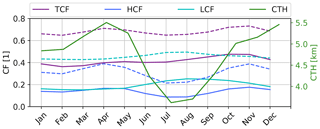
Figure 2 Domain-averaged tropical Atlantic climatologies of TCF, HCF, LCF, and CTH. The dashed lines indicate climatologies of the DARDAR data (June 2006–June 2016) and the solid lines indicate MODIS data (September 2002–June 2017).

3.1 Assessment of the cloud vertical distribution

The ISCCP cloud classification scheme is widely used to simply distinguish between different cloud types using remotely sensed information. The ISCCP is a project, starting in 1982 as part of the World Climate Research Programme (WCRP), with the goal to collect and analyze satellite radiance measurements to infer the global distribution of clouds, the cloud properties, and the cloud diurnal, seasonal, and interannual variations. The clouds are distinguished by their cloud-top pressure (CTP) in hectopascals and their cloud optical thickness. There are three categories for the vertical distribution, namely high (CTP < 440 hPa), middle (≤440 CTP <680 hPa) and low (CTP ≥ 680 hPa). For the computation of MODIS vertical cloud fractions the cloud height category flag from the MODIS 5 km quality assurance (Hubanks, 2015), which is based on the explained ISCCP thresholds, was used to discriminate between the height categories.

Figure 3 (a) Time series of the tropical Atlantic 3-month running mean anomalies of CTH, TCF, HCF, and LCF. Panel (b) is as (a) but comparing the HCF and the Nino3.4 index (NOAA climate prediction center). The Pearson correlation coefficient is found to be −0.53.

3.2 Multiple linear regression

To obtain information of linear changes within the data sets a simple MLRM was developed. For the model development, the time series of the analyzed parameters (y) were assumed to be composed of a constant μ, a seasonal S, a trend (temporal linear change) τ, and a noise η component. These assumptions lead to the following model equation where t stands for time.

$$\begin{array}{}\text{(1)}& y\left(t\right)=\mathit{\mu }+S\left(t\right)+\mathit{\tau }\cdot t+\mathit{\eta }\left(t\right),\end{array}$$

where the seasonal component was specified by the sum of sine and cosine with a period of 12 months.

$$\begin{array}{}\text{(2)}& S\left(t\right)=\sum _{i=\mathrm{1}}^{\mathrm{2}}\sin \left({\displaystyle \frac{\mathrm{2}\mathit{\pi }it}{\mathrm{12}}}\right)+\cos \left({\displaystyle \frac{\mathrm{2}\mathit{\pi }it}{\mathrm{12}}}\right)\end{array}$$

Due to biannual variations in the time series the first harmonic (i=2) of sine and cosine was added to the model.

In a general form Eq. (1) can be written as

$$\begin{array}{}\text{(3)}& y\left(t\right)={\mathit{x}}_t^T\mathit{b}+{\mathit{\eta }}_t,\end{array}$$

where ${\mathit{x}}_t^T$ represents a vector including all explanatory parameters required to describe the parameter y at time step t and b, a vector containing all regression coefficients. In Eq. (4) all possible T linear combinations of the n parameters are summarized in matrix notation.

$$\begin{array}{}\text{(4)}& \left[\mathit{y}\right]=\left[\mathbf{X}\right]\left[\mathit{b}\right]+\left[\mathit{\eta }\right]\end{array}$$

Here y stands for the T×1 vector with the measured parameter for all T months, X for the T×n model matrix including all predictor variables for the estimation for all T months, and b for the n×1 vector containing all the regression coefficients. The variations that are not explained by the model are stored in the T×1 noise vector η.

To find the vector which fits best to the data (denoted as $\widehat{\mathit{b}}$), the ordinary least-square method is used. This method tries to predict the expected parameter $\widehat{\mathit{y}}$ by minimizing the sum of squares of the distances between measured and estimated values. The remaining noise between prediction and measurement is termed residual:

$$\begin{array}{}\text{(5)}& \left[\mathit{\eta }\right]=\left[\mathit{y}\right]-\left[\widehat{\mathit{y}}\right].\end{array}$$

It is important to remember that y is the vector with the measured values and $\widehat{\mathit{y}}$ is the vector containing the values estimated by the model. Consequently, the following expression has to be minimized, in order to minimize the sum of squared residuals:

$$\begin{array}{}\text{(6)}& M=\left|\right|\mathit{\eta }|{|}^{\mathrm{2}}=||\mathit{y}-\left[\widehat{\mathit{y}}\right]|{|}^{\mathrm{2}}={\left[\mathit{\eta }\right]}^T\left[\mathit{\eta }\right].\end{array}$$

Some simplifications and setting the derivation of M with respect to $\widehat{\mathit{b}}$ to zero leads to the final equation to be solved:

$$\begin{array}{}\text{(7)}& \left[\widehat{\mathit{b}}\right]={\left({\left[\mathbf{X}\right]}^T\left[\mathbf{X}\right]\right)}^{-\mathrm{1}}{\left[\mathbf{X}\right]}^T\left[\mathit{y}\right].\end{array}$$

A more detailed explanation of the used MLRM can be found in Wilks (2011).

4 Results

4.1 Monthly means and climatologies

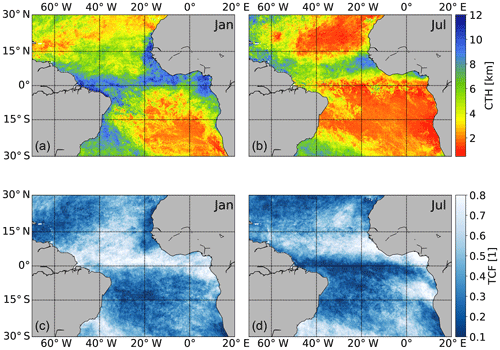
In Fig. 1 the monthly means for January (left) and July (right) 2009 are displayed for the CTH (upper panels) and the TCF (lower panels) for the investigated spatial domain of the tropical Atlantic. Near the Equator the data reveal a band with high cloud tops and high cloud amounts indicating the intertropical convergence zone (ITCZ). Furthermore the seasonal shift of the ITCZ is represented. Lower cloud tops due to the well-known trade wind inversion are predominant in the trade wind regions. The stratocumulus region near the coast of Angola and Namibia with higher CF and low CTH is illustrated in the data as well. In boreal winter (left) a part of the south Atlantic convergence zone can be identified southeast of Brazil with high cloud tops and high cloud amounts.

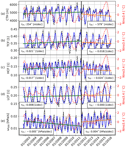
Figure 4 Quantification of temporal linear changes in the tropical Atlantic mean associated with ENSO phase transition. (a) CTH, (b) TCF, (c) HCF, (d) LCF, and (e) ω₅₀₀. The MODIS data are displayed in black, and in blue the applied MLRM are shown. In red the Nino3.4 index is displayed.

The tropical Atlantic domain-averaged climatologies (see Sect. 2) of the CTH and the vertically resolved CFs are shown in Fig. 2.

The CTH climatologies vary between 3.6 km in boreal summer and 5.5 km in boreal spring and in December. The climatologies of the CFs show that the MCF is very low (not shown) and the TCF is approximately composed for the same portion of LCF and HCF. The HCF is in phase with CTH showing similar seasonal variability. For any interpretation of averaged CTH its strong non-Gaussian character is important to take into account. The climatologies calculated for the DARDAR data (June 2006–June 2016) reflect the same seasonal variability; indeed they have a positive bias (∼ 0.2) towards higher CFs, which can be explained with the higher sensibility of lidar for high, optically thin clouds and by multilayer conditions as DARDAR can observe both high and low clouds in one column.

4.2 Anomalies

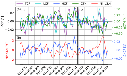
To gain insights into the interannual variability and the temporal evolution of the variables, the monthly tropical Atlantic 3-month running mean anomalies (see Sect. 2) were analyzed. As illustrated in Fig. 3 the mean anomalies of CTH are strongly positively correlated with the HCF anomalies, with a Pearson correlation coefficient (PCC) of 0.89 and an R² value (coefficient of determination) of 0.8. The interannual variability of CTH is mainly driven by the HCF. The time series of the CTH and the HCF show phases with negative anomalies around 2002, at the end of 2009, and at the end of the period starting in 2015 and phases with positive anomalies between 2007 and 2008 as well as between 2010 and 2011 (see Fig. 3). Remarkable is the large anomaly of the CTH and HCF at the end of the time series, which is not present in the TCF and LCF. The time periods where the anomalous phases occur indicate a link to the ENSO. An impact of ENSO on the tropical Atlantic ocean–atmosphere system is well known even though the exact mechanism of teleconnection is still not fully understood. Positive ENSO events were found to be associated with higher SSTs in the tropical Atlantic (Klein et al., 1999), a weakening of the Walker circulation and the Atlantic Hadley circulation (e.g., Klein et al., 1999; Wang, 2004), and a stronger vertical wind shear over the tropical Atlantic (Zhu et al., 2014). Figure 3b displays the 3-month running mean of the HCF anomaly and additionally the Nino3.4 index (obtained from the NOAA climate prediction center). The interannual variability of the mean HCF at the tropical Atlantic and the Nino3.4 index are negatively correlated ($\mathrm{PCC}=-\mathrm{0.53}$). As shown in Marchand (2013) a strong negative correlation between ENSO and high-cloud amount is also present in MODIS (and the Multi-angle Imaging SpectroRadiometer, MISR) observations in the Tropical Warm Pool region (ocean between 30^∘ N–30^∘ S and 100–160^∘ E), the Indian Ocean, and the tropical western and central Pacific. Due to the strong ENSO influence, two phases with temporal linear change can be distinguished within the investigated time period. The phases are related to a transition from more El Niño-like to more La Niña-like conditions (phase 1) and vice versa (phase 2). For phase 1 from September 2002 (El Niña event) to the end of 2011 (La Niña event) an increase and for phase 2 from the end of 2011 to 2016 (strong El Niño event) a decrease in the high-cloud amount were found.

4.3 Multiple linear regression analysis

In order to quantify possible linear changes in the investigated variables associated with a warming ocean and changes in atmospheric dynamics due to climate change, the multiple linear regression model was applied to the domain-averaged variables. In attempting to account for effects caused by the ENSO we included the Nino3.4 index as an explanatory parameter in the MLRM described in Sect. 3.2 for this analysis. For the analyzed time period significant (p value < 0.05) linear changes were found for the domain-averaged CTH (−178 m per decade), HCF (−0.0006 per decade), and the LCF (0.001 per decade) (not shown). The time series (especially CTH and HCF) are highly influenced by the ENSO. The main reason for this may mainly be the changes in the atmospheric large-scale dynamics due to the eastward shift of the Walker circulation during positive ENSO phases (e.g., Philander, 1989; Bayr et al., 2014).

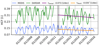
Figure 5 Comparison of the tropical Atlantic domain average of the 2^∘ × 2^∘ DARDAR (green) and MODIS (blue) HCF monthly means.

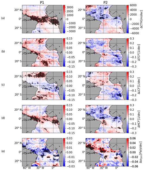
Figure 6 Temporal linear changes of CTH, TCF, HCF, and LCF for every 0.2^∘ × 0.2^∘ grid box. On the left are the temporal linear changes for phase 1 and on the right are temporal linear changes for phase 2. The dots indicate that within a grid box of 1^∘ × 1^∘, more than half of the temporal linear changes were statistically significant.

During the investigated time period, the analysis revealed opposing linear changes that are mostly related to transitions between more positive and negative ENSO conditions (see Fig. 4). Therefore we decided in the next step to separate the analysis into two phases and apply the model to both phases separately. This analysis is thought to be a first step of quantifying the linear changes in the cloud vertical distribution associated with ENSO phase transition, using satellite data. This is especially valid for the second phase where a clear transition from negative to strong positive ENSO conditions occurred (Fig. 4). For this analysis we used the MLRM explained in Sect. 3.2. To find the best separation of the phases the maximum of the sum of the explained variances of the two models was calculated for differing phase separations. The best fit was found for the period from September 2002 to November 2011 (P1) and the period from November 2011 to June 2016 (P2). The changes in P1 are mainly associated with a large La Niña event (2010) at the end of P1 and that in P2 with a large El Niño event (2015) at the end of P2. Figure 4 illustrates the results of the regression analysis applied to the tropical Atlantic mean for the different variables.

The CTH in Fig. 4a and the HCF in Fig. 4c show a significant El Niño-related CTH decrease in P2 of −579 m per decade and of −0.024 per decade for HCF. This indicates that observed changes in the CTH are mainly due to changes in high-cloud amount. The LCF (d) shows neither significant changes in P1 nor in P2. The changes of the TCF in P2 are visible, but statistically not significant (b). In P1 all variables (a–d) show a linear increase that is significant, except for the LCF.

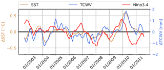
Figure 7 Time series of the tropical Atlantic 3-month running mean anomalies of SST (orange) and TCWV (blue). In red the qualitative progress of the Nino3.4 index is shown.

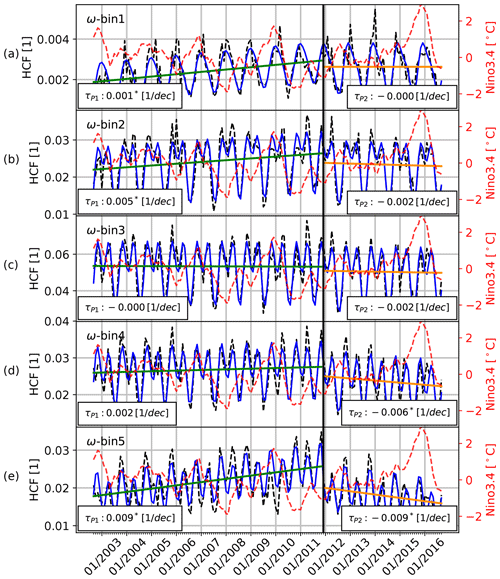
Figure 8 Time series of the tropical Atlantic domain-averaged HCF for different ω bins. (a) ω bin 1, (b) ω bin 2, (c) ω bin 3, (d) ω bin 4, and (e) ω bin 5.

To evaluate the anomalies observed with the passive MODIS instrument, DARDAR data (see Sect. 2.2) from active lidar and radar instruments were analyzed. Due to the low sampling, monthly means were computed and compared to MODIS with a 2^∘ × 2^∘ resolution. As Fig. 5 illustrates, the seasonal and interannual variability of the HCF, as well as its decrease (−0.073 per decade, not significant) in P2, is visible in the DARDAR data as well despite the low sampling. As already seen in the climatologies (Fig. 2) DARDAR has a positive offset.

To obtain spatial information of the anomalies (temporal linear changes) the MLRM was applied to every 0.2^∘ × 0.2^∘ grid box. Figure 6 displays the linear part of the MLRM τ. The CTH (a) and the HCF (d) show very similar patterns in both phases with significant increases between ±10^∘ N–S in P1 and significant decreases between 0 and 20^∘ N in P2 confirming the strong link between changes in CTH and the HCF. For the TCF (b) a significant decrease in P2 at the stratocumulus region near the coast of Angola and Namibia, which is mainly caused by a decrease in LCF (c), is visible. The HCF and the LCF have opposing patterns that cause most of the signal in TCF to be extinguished. This endorses the idea of looking at the cloud vertical distribution rather than just at total cloud amount in climate studies.

4.4 Link between tropical Atlantic and ENSO

Table 1 Definition of the ω₅₀₀ bins.

During a positive ENSO phase the anomalous high SST in the Pacific induces an average warming of the tropical Atlantic troposphere, e.g. trough Kelvin waves causing an increase in the meridional tropospheric temperature gradient (e.g., Horel and Wallace, 1981; Yulaeva and Wallace, 1994; Chiang and Sobel, 2002; Zhu et al., 2014). This leads to an increase in the vertical wind shear (e.g., Aiyyer and Thorncroft, 2006; Shaman et al., 2009; Zhu et al., 2014) and tends to increase the static stability over the tropical Atlantic (e.g., Tang, 2004; Larson et al., 2012). Moreover, a weakening of the Atlantic Hadley and Walker circulations and an eastward shift of the latter (Philander, 1989; Klein et al., 1999; Wang, 2006) are associated with higher Pacific SSTs. Furthermore, a reduction in equatorial Atlantic rainfall (Saravanan and Chang, 2000; Chiang and Sobel, 2002), a lagged SST increase caused by a warmer troposphere, and reduced latent and sensible heat losses due to weaker trade winds and a reduction in cloudiness (Curtis and Hastenrath, 1995; Enfield and Mayer, 1997; Klein et al., 1999; Saravanan and Chang, 2000; Huang, 2002) were found during El Niño. The reduction in cloudiness leads to changes in radiation fluxes due to higher absorption of solar radiation by the ocean, which in turn increases the mean tropical Atlantic SST (Curtis and Hastenrath, 1995; Klein et al., 1999), strengthening the positive SST feedback between the Pacific and the Atlantic. In general the described effects are observed to be inverted during La Niña. As our analysis of MODIS data shows that the decrease in TCF during time periods dominated by El Niño events is observed to be mainly caused by a decrease in high clouds (Sect. 4.2 and 4.3), the cloud radiative forcing might be negative, counteracting the increase in tropical Atlantic SST.

The analysis of AMSR-E-retrieved SST and TCWV data shows a consistent (e.g., Klein et al., 1999) 3-month-delayed tropical Atlantic SST and TCWV increase after an El Niño event (Fig. 7). Furthermore, a significant positive trend of 0.3 ^∘C per decade was found for the regional mean SST.

To investigate to what extent the observed anomalies in HCF are linked to ENSO-induced changes in the large-scale circulation over the tropical Atlantic, the large-scale vertical velocity ω at 500 hPa acquired from ERA-Interim data was analyzed. The results are illustrated in Fig. 4c for the tropical Atlantic mean and in Fig. 6e for the grid-box-based analysis. ω is negatively defined so that negative velocities imply upward movements and vice versa. For the tropical Atlantic mean a decrease in P1 and an increase in P2 were found. The anomalies are mostly due to strengthening/weakening in upward movement rather than weakening/strengthening in downward movement. This is coherent with the results of the grid-box-based analysis displayed in Fig. 6e where in both phases the largest and most of the significant anomalies are found in the ITCZ region where upward movement predominates.

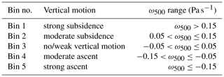
The comparison of ΔHCF (Fig. 6d) and Δω₅₀₀ (Fig. 6e) reveals similar patterns for both phases. The increase/decrease in the high-cloud amount in P1/P2 seems to be mainly associated with an increase/decrease in large-scale upward motion in the equatorial Atlantic Ocean. A stratification of the HCF into different ω₅₀₀ bins as listed in Table 1 confirms that the decrease in the high-cloud amount in P2 occurs in regions with strong upward movements; see Fig. 8d and e. This supports the idea that the observed anomalies, particularly the decrease in CTH and HCF in P2, are caused by an ENSO-induced change in large-scale atmospheric motion due to, for example, an eastward shift of the Walker circulation and a weakening of the Walker and the Atlantic Hadley cell, and this indicates an increased vertical stability and vertical wind shear.

5 Summary and conclusion

In this study the Moderate Resolution Imaging Spectroradiometer (MODIS) (aboard Aqua) cloud products were used to analyze the interannual variability of the cloud vertical distribution at the tropical Atlantic for a period of 14 years (2002 to 2016). Furthermore, the influence of the transition from one El Niño–Southern Oscillation (ENSO) phase to another on the tropical Atlantic cloud vertical distribution was analyzed and quantified. Based on level 2 data, daily composites on a 0.1^∘ × 0.1^∘ regular grid were generated. For the analysis, 0.2^∘ × 0.2^∘ monthly means, calculated on the basis of the daily composites, were used. The data represented large circulation patterns such as the band with high cloud tops and cloud amount in the ITCZ and its seasonal shift well. Also, the trade wind inversion regions with their characteristic low cloud tops and the broad stratocumulus region on the west coast of Namibia were represented in the data.

Furthermore, sea surface temperature (SST) and total column of water vapor (TCWV) data from the AMSR-E (2002–2011) were analyzed. The data showed a significant positive trend in SST of 0.3 ^∘C per decade and a 3-month lagged increase in SST and humidity during El Niño, which is consistent with the literature  (e.g., Curtis and Hastenrath, 1995; Klein et al., 1999).

For the investigated 14 years, significant linear changes were found for the domain-averaged cloud-top height (CTH) (−178 m per decade), high-cloud fraction (HCF) (−0.0006 per decade), and low-cloud fraction (LCF) (0.001 per decade). Furthermore, the analysis of the time series revealed strong interannual variability of the vertical cloud distribution, which was found to be well correlated with changes in the large-scale atmospheric circulation (ω at 500 hPa) due to ENSO-associated teleconnective causes. The changes in the large-scale circulation might be associated with the eastward shift and the weakening of the Walker circulation and a weakening of the Hadley cell during El Niño conditions. The largest ENSO-linked anomalies were found for the HCF, which also drives the observed anomalies in the mean CTH. For the transition from more La Niña-like to more El Niño-like conditions, a decrease in tropical Atlantic HCF, mainly at the equatorial ITCZ influenced region, was observed and was linked to a decreasing large-scale vertical upward movement by including ERA-Interim reanalysis data (ω at 500 hPa). The HCF and LCF showed opposite behavior, which might mask much of a possible signal if using solely total cloud fraction. This supports the efforts to consider the vertically resolved cloud fraction rather than the cloud fraction as a whole. The decrease in cloudiness is consistent with findings from Klein et al. (1999).

In addition to other factors such as alleviated surface wind speed and a warmer troposphere, the change in cloud cover is associated with positive SST anomalies (e.g., Klein et al., 1999). Subsequently, a sensitivity study of the cloud radiative forcing associated with ENSO-linked changes could be performed to quantify the influence of radiation changes. As the anomalies in CF are found to be mainly driven by changes in the high-cloud amount, the radiative impact on tropical Atlantic SST might be negative during El Niño conditions.

As most of the climate projections show a shift towards more El Niño-like conditions and similar changes in the tropical Atlantic circulation (e.g., Vecchi and Soden, 2007; Bayr et al., 2014; Hu et al., 2018), satellite observations of large ENSO events in combination with model data could be furthermore used as a large “experiment” for possible effects of global warming on ocean–atmosphere dynamics and cloud radiative forcing.