the Creative Commons Attribution 4.0 License.
the Creative Commons Attribution 4.0 License.
 | 14 Jun 2024
California wildfire smoke contributes to a positive atmospheric temperature anomaly over the western United States
Robert J. Allen
King-Fai Li
Wildfires in the southwestern United States, particularly in northern California (nCA), have grown in size and severity in the past decade. As they have grown larger, they have been associated with large emissions of absorbing aerosols and heat into the troposphere. Utilizing satellite observations from MODIS, CERES, and AIRS as well as reanalysis from MERRA-2, the meteorology associated with fires during the wildfire season (June–October) was discerned over the nCA-NV (northern California and Nevada) region during the period 2003–2022. Wildfires in the region have a higher probability of occurring on days of positive temperature (T) anomalies and negative relative humidity (RH) anomalies, making it difficult to discern the radiative effects of aerosols that are concurrent with fires. To attempt to better isolate the effects of large fire emissions on meteorological variables, such as clouds and precipitation, variable anomalies on high fire emission days (90th percentile) were compared with low fire emission days (10th percentile) and were further stratified based on whether surface relative humidity (RHs) was anomalously high (75th percentile) or low (25th percentile) compared with typical fire season conditions. Comparing the simultaneously high fire emission and high RHs data with the simultaneously low fire emission and high RHs data, positive tropospheric T anomalies were found to be concurrent with positive AOD anomalies. Further investigation found that due to shortwave absorption, the aerosols heat the atmosphere at a rate of 0.041 ± 0.016 to 0.093 ± 0.019 K d−1, depending on whether RH conditions are anomalously positive or negative. The positive T anomalies were associated with significant negative 850–300 hPa RH anomalies during both 75th percentile RHs conditions. Furthermore, high fire emission days under high RHs conditions are associated with negative CF anomalies that are concurrent with the negative RH anomalies. This negative CF anomaly is associated with a significantly negative regional precipitation anomaly and a positive net top-of-atmosphere radiative flux anomaly (a warming effect) in certain areas. The T, RH, and CF anomalies under the simultaneously high fire emission and high RHs conditions compared with the simultaneously low fire emission and high RHs conditions have a significant spatial correlation with AOD anomalies. Additionally, the vertical profile of these variables under the same stratification is consistent with positive black carbon mass mixing ratio anomalies from MERRA-2. However, causality is difficult to discern, and further study is warranted to determine to what extent the aerosols are contributing to these anomalies.
- Article
(10231 KB) - Full-text XML
-
Supplement
(10660 KB) - BibTeX
- EndNote


As a result of climate change, land use change, and forest management, the frequency of wildfires in California has trended upward from 100 fires per year in the 1920s to 300 fires per year in the late 2010s (Li and Banerjee, 2021). The size of these wildfires has also increased, with total burned area (square distance burned by a fire) increasing from roughly 1000 to almost 4000 km2 in the same period (Li and Banerjee, 2021). According to a recent study, the frequency of extreme daily wildfire events in the region is projected to increase by 59 %–172 % in coming years due to climate change (Brown et al., 2023), which is consistent with findings of numerous other studies (Palinkas, 2020; Ager et al., 2021; United Nations Environment Programme, 2022). In both higher and lower CO2 mitigation scenarios, large wildfire events are projected to become more commonplace by the end of the 21st century worldwide as well as in the southwestern US (United Nations Environment Programme, 2022). Large wildfire events in the late 2010s and early 2020s were associated with more intense “fire weather”: high temperature (T), low relative humidity (RH), and high surface wind speeds (Us) (Varga et al., 2022; Keeley and Syphard, 2019). These fire weather conditions may be potentially intensified, or alleviated, by the fires themselves. Higher burn severity wildfires, such as the 2020 wildfires in California (CA), have been observed to inject smoke plumes higher into the troposphere than in previous years (Wilmot et al., 2022). These smoke plumes consist of both shortwave (SW) absorbing aerosols such black carbon (BC) and reflective aerosols such as organic aerosol (OA) as well as brown carbon, which is absorbing and reflective. Additionally, wildfires have also been associated with emissions of other aerosol species through feedbacks. While dust is not emitted from biomass burning, a number of studies have linked fires to concurrent dust emissions through the creation of convective updrafts (Wagner et al., 2018, 2021) and delayed dust emissions through wildfire clearing of vegetation (Wagenbrenner et al., 2013, 2017; Yu and Ginoux, 2022). The absorbing properties of wildfire smoke and co-emitted dust over the western US, measured using absorbing aerosol optical depth (AAOD), is uncertain. However, a recent study of CA fires indicates that wildfires increase AAOD relative to the annual mean by 10-fold (Cho et al., 2022). An injection of absorbing aerosols into the troposphere may cause a local warming affect, altering the hydrological and radiative balance of the atmosphere (Allen and Sherwood, 2010; Thornhill et al., 2018; Allen et al., 2019; Herbert and Stier, 2023). Smoke plumes that reach the upper troposphere (pressures < 500 hPa) may deposit absorbing aerosols that could burn off high clouds and promote more stable low clouds (Stjern et al., 2017; Smith et al., 2018; Allen et al., 2019), leading to SW and longwave (LW) cooling. Alternatively, if the absorbing aerosols are concurrent with low clouds, the relative humidity of the liquid cloud layer would be decreased, burning off low clouds and leading to a decrease in outgoing SW flux (Koch and Del Genio, 2010; Allen and Sherwood, 2010). These are both examples of aerosol semi-direct effects. Past observations and modeling experiments have shown dust aerosol is associated with semi-direct effects (Tsikerdekis et al., 2019; Amiri-Farahani et al., 2017; Helmert et al., 2007), as dust also has SW absorbing properties (Highwood and Ryder, 2014; Kok et al., 2023). Furthermore, the higher altitude of absorbing aerosol from California fires may alter cloud microphysics, which also has the potential to change the radiative balance of the surface and atmosphere. An influx of aerosols into the troposphere may create an abundance of cloud condensation nuclei (CCN) for droplets to condense onto, decreasing the effective radius (Reff) of the clouds – an effect already observed with smoke (OA and BC) particles in the northwestern US (Twohy et al., 2021). A decrease in Reff would increase the albedo of the clouds, assuming a constant water path, which would then increase outgoing SW radiation. This decrease in Reff can also affect the liquid water path (LWP), as the smaller droplets can evaporate much faster than larger droplets or the smaller droplets can suppress precipitation, which increases LWP by reducing the liquid water leaving the cloud (Goren and Rosenfeld, 2012). The lighter droplets can also be lofted higher in the atmosphere, where they condensate further and release latent heat, then eventually fall from this greater height and evaporate. Therefore, to compensate, polluted clouds have more intense updrafts and downdrafts than pristine clouds (Khain, 2009). SW absorption itself can also decrease precipitation (P) in other ways, such as reducing SW radiation reaching the surface or through rapid atmospheric adjustments (Sand et al., 2020; Samset, 2022; Allen et al., 2023).
Large fires are not limited to the western US only. Australia, the Mediterranean Basin, and South America have all experienced an increase in large fire events due to climate change and land management (Shi et al., 2021; Ruffault et al., 2020; Artaxo et al., 2013; Allen et al., 2024a). As the western US, and other parts of the world, enter this new regime of large fires, the need arises for an improved understanding of the effects of aerosols emitted primarily (through biomass burning), secondarily (oxidation of emitted volatiles), or through feedbacks (such as dust emissions concurrent with fires) by wildfires. Models participating in the Coupled Model Intercomparison Project version 6 (CMIP6) (Eyring et al., 2016) do not have parameterizations of biomass burning (BB) aerosol emissions that respond to CO2 emissions in most of their experiments, including the DECK (Diagnosis, Evaluation, and Characterization of Klima) experiments (Gomez et al., 2023). The models that have interactive BB aerosol emissions tend to parameterize them as a function of fuel flammability (temperature and moisture), fuel density, and plant functional type (Mangeon et al., 2016; Li et al., 2019). Most models participating in CMIP6 do not have dynamic vegetation models (Li et al., 2019) and therefore are incapable of incorporating fire–dust feedbacks. Instead, modelers rely on the prescription of BB aerosols in most experiments.
Recent modeling experiments have found significant effects of wildfires on regional and global climate scales. Previously, using prescribed aerosol simulations in the Community Earth System Model version 2 (CESM2), it was shown that the large 2019 wildfires in Australia could have intensified that year's La Niña through aerosols directly cooling the ocean surface (Fasullo et al., 2021). Another CMIP6 study observed a similar effect on La Niña as a result of a teleconnection caused by an influx of absorbing aerosols into the atmosphere from South African wildfires (Amiri-Farahani et al., 2020). Biomass burning aerosols may also have other effects on large-scale ocean circulation, such as an invigoration of the Atlantic Meridional Overturning Circulation (Allen et al., 2024b). As far as the southwestern US is concerned, a modeling experiment using the WRF/CHEM model was run to analyze the effects of a wildfire event on weather forecasts (Chen et al., 2014). This study found that the BB aerosols suppressed convection, prevented cloud formation, and decreased precipitation. While studies such as these demonstrate that it is possible to model past effects of fires on local and global climate, without parameterization of BB aerosol emission, as well as parameterization of secondary dust aerosol emission from wildfire-cleared vegetation, the radiative forcing of the primary and secondary aerosols of future fires will remain a source of uncertainty. Furthermore, there are few, if any, studies that attempt to discern the impacts of large fires over the southwestern US. Twohy et al. (2021) analyzed satellite observations of cloud microphysical properties over part of the region; however, their study was conducted during only one wildfire event in 2018. As a result, there is no comprehensive long-term observational study over the southwestern US concerning wildfire aerosol–cloud interaction. Therefore, to further understand the effects of wildfires on the climate of one of the most populated areas in the US, this paper aims to identify the radiative and microphysical effects that these aerosols may have in the region under different atmospheric conditions utilizing satellite data.
The objective of this study is to quantify the impacts of wildfire aerosol emissions on meteorological parameters, such as clouds and precipitation, over the southwestern US using observations. This includes the Aqua satellite with the MODIS, AIRS, and CERES instruments. The Modern-Era Retrospective analysis for Research and Applications version 2 (MERRA-2) reanalysis project (Randles et al., 2017; Global Modeling And Assimilation Office and Pawson, 2015) is used to obtain daily black carbon mass mixing ratio vertical profiles. Fire dry matter (DM) emission data are used as a proxy for fire severity and are derived from the Global Fire Emissions Database 4.1s (GFED4.1s) (van der Werf et al., 2017; Randerson et al., 2017). All datasets are globally gridded observational datasets, with the exception of GFED4.1s and MERRA-2, which are considered globally gridded reanalysis datasets.
2.1 Global Fire Emissions Database (GFED4.1s)
GFED4.1s DM emissions are calculated in the Carnegie–Ames–Stanford Approach (CASA) model, which requires MODIS burned area data, meteorological data from the ERA-Interim reanalysis dataset, photosynthetically active radiation data based on Advanced Very High Resolution Radiometer satellite instrument retrievals, and vegetation continuous field data from the MODIS MOD44B dataset (van der Werf et al., 2017). DM is the emission of any gas or aerosol from burned vegetation, and a list of all these types of emissions can be found in van der Werf et al. (2017). The CASA model is run using burned area data from combined MODIS–Aqua and MODIS–Terra level 3 data (MCD64A1). Wildfire studies tend to use either fire power (from MODIS or VIIRS) or burned-area-based datasets to quantify fire severity. Burned area is determined by MODIS from a time series of the burn-sensitive vegetation index, which compares daily surface reflectances (Giglio et al., 2018). Fire power is the radiated energy from fires over time, and MODIS determines this quantity by comparing the brightness temperature of a fire pixel with the background brightness temperature (Peterson et al., 2013). Use of a burned-area-based dataset is preferable to a fire power dataset for this paper, as cloud cover may obstruct fire power data retrievals, leading to an underestimation of fire size and/or severity in a given time period. While cloud cover can also block burned area retrievals, burned area can be recorded once cloud cover has been dissipated, unlike fire power. This introduces a temporal uncertainty, however. This temporal uncertainty is ±1 d for clear-sky conditions, ±5 d under consistent 75 % cloud cover, and up to ±20 d over persistently very cloudy (85 % or higher) intervals (Giglio et al., 2013). However, this temporal uncertainty is likely of little significance for this paper, as cloud cover over the western US during the wildfire season is rarely persistently high (aside from “June gloom” in coastal regions), and the lifetime of biomass burning aerosols (roughly 4–12 d) is generally greater than or equal to the temporal uncertainty of clear-sky or consistently cloudy burned area data (Cape et al., 2012). The daily underestimation of fire power is demonstrated in Fig. S1 in the Supplement, which indicates that Aqua fire power retrievals, taken from the MYD14A1 dataset (Giglio and Justice, 2015), underestimate daily fire severity compared to DM, with 98 % of days reporting a lower normalized fire power than normalized DM. Therefore, for fire power to be a more useful metric, a daily combined Aqua/Terra/VIIRS dataset would have to be used, which is not available for the period of interest. GFED4.1s fire emissions are also preferred over fire power data and raw burned area data, as the calculation of fire emissions takes vegetation type and net primary production into account. Raw burned area and fire power datasets yield information about fire size and intensity, but as aerosol emission also depends on the type of vegetation being burned, use of either dataset over a fire emission dataset may underestimate or overestimate the impact of biomass burning aerosols on clouds. However, the use of GFED4.1s data has drawbacks. While the use of burned area data reduces the chance of an underestimation of fire impacts, the previously mentioned temporal uncertainty is introduced. Additionally, the CASA model itself is associated with uncertainties. Calculation of net primary production in the model, for example, does not take meteorological variables into account (Liu et al., 2018). As a result, caution must be taken when analyzing the results. To ensure results are robust, the GFED4.1s DM stratification method was verified by analyzing MODIS AOD anomalies (see Sect. 2.2) during large fire events (Sects. 3.3, 4.2) and by performing cross correlations between AOD and DM (Sect. S1 in the Supplement, Fig. S2). GFED4.1s emissions and burned area data are available from 1997 to 2016. Data for the period 2017–2022 are also available, but the data are in “beta” and therefore are more limited. Both the complete and the beta data contain total carbon emissions as well as dry matter emissions. GFED4.1s also estimates the contribution of six different types of vegetation biomes (boreal forest, temperate forest, grassland, agriculture, peat, and tropical forest) to the carbon and dry matter emissions. However, the beta dataset only estimates these contributions for DM. Therefore, DM is used as a proxy for the severity of the emissions of a given fire, as it is the only variable that both the complete and beta data contain and speciate. All observational datasets utilized in this study have a 1° resolution; however, the GFED4.1s emission data are of a 0.25° resolution. Therefore, these data were regridded to a 1° grid. It should be noted that GFED5 has recently been released (Chen et al., 2023); however, this dataset was not used as it does not yet include emissions but only has data available up to 2020, and it was released after analysis for this paper had concluded.
2.2 Aqua
MODIS-Aqua. Cloud and aerosol optical depth (AOD) data were derived from Moderate Resolution Imaging Spectroradiometer (MODIS) level 3 data. Specifically, the MODIS collection 6.1 1° level 3 product (MYD08_D3) (Platnick et al., 2003; Salomonson et al., 2002; MODIS Atmosphere Science Team, 2017) is utilized, which yields daily retrieval products from the Aqua satellite. The Aqua satellite makes two overpasses for the region of interest: one ascending run from 14:00 to 15:00 LT (local time; all instances of time in the text are in local time and one descending run from 02:00 to 03:00. The descending dataset is used, as most MODIS level 3 cloud property products provided are descending (morning) only. For MODIS cloud retrievals during periods of large AOD, especially when the aerosols are concurrent with clouds, it is possible for MODIS to misidentify aerosols as clouds (Herbert and Stier, 2023). This may cause errors in cloud property retrievals as well as an overestimation of cloud fraction (CF). This may lead to overestimation of CF during anomalously large fire events. While the MODIS Dark Target and Deep Blue AOD algorithms are extensively quality controlled and evaluated (Levy et al., 2013; Platnick et al., 2017; Wei et al., 2019), there is still room for error in AOD and cloud retrieval. Additionally, as it is not possible to distinguish wildfire AOD from other AOD, whenever possible, fire emissions from GFED4.1s are used to discern the impacts of fires on cloud properties.
AIRS. Data concerning T, water mass mixing ratio , CF, and RH profiles, as well as surface temperature Ts and surface relative humidity RHs, were derived from Atmospheric Infrared Sounder (AIRS) level 3 daily data (AIRS3STD) (AIRS Science Team and Texeira, 2013). As with the MODIS data, the descending dataset is used.
CERES. Top-of-atmosphere as well as in-atmosphere radiative flux data were derived from Clouds and the Earth's Radiant Energy System (CERES) level 3 daily 1° Synoptic product (SYN1deg-Day) (NASA/LARC/SD/ASDC, 2015, 2017, 2023). This is a combined Terra and Aqua dataset for the period 2002–2021, and for 2022 it is a combined Terra and NOAA-20 dataset. This CERES dataset combines cloud data from MODIS/VIIRS, aerosol data from GEOS, and top-of-atmosphere radiative flux data from CERES to produce all-sky, clear-sky, and aerosol-free radiative flux profiles.
2.3 GPCP combined precipitation dataset
P data for this project were derived from the daily Global Precipitation Climatology Project (GPCP daily) Climate Data Record version 1.3 dataset (Huffman et al., 2001; Adler et al., 2018). GPCP combines satellite observations as well as rain gauge data to produce 1° daily precipitation amount data.
2.4 MERRA-2 aerosol profiles
Daily vertical black carbon aerosol mass mixing ratio profiles are derived from the M2I3NVAER data product (Global Modeling And Assimilation Office and Pawson, 2015; Buchard et al., 2015). This product estimates aerosol profiles by assimilating MODIS AOD into the GEOS5 model, which is radiatively coupled with the Goddard Chemistry, Aerosol, Radiation, and Transport (GOCART) aerosol module. The GOCART model includes biomass burning emissions from the NASA Quick Fire Emission Dataset (QFED) version 2.1, which provides daily biomass burning aerosol estimates (Buchard et al., 2015). These profiles were then validated using ground and satellite observations of aerosol profiles. This dataset has been previously used to determine effects of wildfire aerosols in other parts of the world (Raga et al., 2022; Nguyen et al., 2020). The aerosol profiles are archived in a high-resolution hybrid sigma pressure grid and therefore must be interpolated into 1° grid cells and converted into traditional pressure levels. For the purposes of this paper, only the black carbon variables are analyzed. MERRA-2 separates BC into two types: hydrophobic black carbon (BCpho) and hydrophilic black carbon (BCphi).
2.5 CALIPSO
The Cloud-Aerosol Lidar and Infrared Pathfinder Satellite Observation satellite (CALIPSO) provides observations of aerosol extinction coefficient profiles. MERRA-2 profiles are utilized in the main analysis instead of CALIPSO profiles, as gridded CALIPSO data are of too low resolution and are monthly as opposed to daily. Additionally, CALIPSO started collecting data in 2006, which makes the satellite not temporally consistent with MODIS and AIRS, which started collecting data in 2002. More information on CALIPSO can be found in Sect. S2.
3.1 Statistics
The bulk of the analysis for this paper involves empirical cumulative distribution functions (CDFs). Empirical distribution functions are calculated for each variable of interest under differing fire and meteorological conditions, and the shift in each distribution is compared. Plotting two CDFs on the same axis allows for comparison on how likely an anomaly is to be positive or negative under differing circumstances, such as how likely a positive or negative anomaly for a certain variable is to occur during a high (90th percentile) fire dry matter emission (DM90) or low (10th percentile) fire dry matter emission (DM10) event. The 90th percentile is chosen, as the purpose of this paper is to analyze the effects of large fire events on climate, not the effects of fires in general. From the calculated normal distributions, the effect size of one variable's distribution on another variable's distribution is estimated using Cohen's d. Cohen's d is an approximation of by how many standard deviations (σs) the distribution shifts in response to a change in a variable. In this paper, d is calculated to determine the effect size of DM on other variables. Here, d is approximated using
where is the mean of the (DM90) group (group a), and is the mean of the (DM10) group (group b), σa is the standard deviation of group a, and σb is the standard deviation of group b. d= 0.2–0.5 is considered to be a weak effect, d= 0.5–0.8 is a moderate effect, and d= 0.8 or higher is classified as a strong effect.
When comparing two datasets, a two-tailed pooled t test is used to assess significance, where the null hypothesis of a zero difference is evaluated, with n1+n2−2 degrees of freedom, where n1 and n2 are the number of elements in each dataset, respectively. Here, the pooled variance
is used, where S1 and S2 are the sample variances. For the purposes of this project, the t test is evaluated at 90 % significance.
3.2 Data stratification and comparison
In Sect. 3.1, it was mentioned that CDFs for variable anomalies during anomalously high and low DM emission events are generated to discern to what degree fires impact these anomalies. The purpose of this stratification, particularly stratification of days into anomalously high and low fire events, is to isolate the effects of fires on clouds and/or weather. The remainder of this section will detail how data stratification is accomplished. First, a variable is chosen for analysis (such as CF). Next, this variable as well as the variables that are used to stratify the variable are filtered to include only the region of interest. As the Aqua satellite does not record data for each grid cell at every time step, wherever a coordinate (latitude, longitude, time) is missing a value for a specific variable, the variable(s) it is being stratified by also has the value at that coordinate replaced by a missing value (and vice versa). Next, to focus on potential feedbacks fires may have on land, a land–sea mask is applied. Then, the daily regional anomaly for each variable is taken. Subsequently, the 2003–2022 wildfire seasons are spliced together, which results in a time series of roughly 3060 d. From this 3060 d time series, any days with no data are removed. Next, the average of each day of the wildfire season is removed from each data point in the distribution to give a time series of anomalies for each variable. Booleans that filter out days above or below a certain percentile for the stratification variables are then applied simultaneously. For each dataset, an empirical CDF is then calculated. Following this, the means are differentiated from each other to determine whether the stratification variable (such as DM) leads to a significant change in the variable anomaly in question. This process can be applied both for a regional average and on a grid cell-by-grid cell basis. When this process is performed on a grid cell-by-grid cell basis, the Pearson cross-correlation coefficient r is determined by spatially correlating the stratified variables with one another. This helps determine whether one change in a variable as a result of fires (or other factors) feeds back onto another to cause a change in anomaly. Figure 1 serves as a verification of the stratification method and validation of GFED4.1s emissions data. Monthly cross-correlation analysis (Sect. S1, Fig. S2) as well as previous works (Wilmot et al., 2022; Schlosser et al., 2017; Cho et al., 2022) indicate that during large fire events, AOD and/or particulate matter concentrations are significantly larger compared with no fire conditions. The significant increase in AOD over most of the southwestern US supports the assertion that GFED4.1s fire emissions are an acceptable indicator of large fire occurrences.
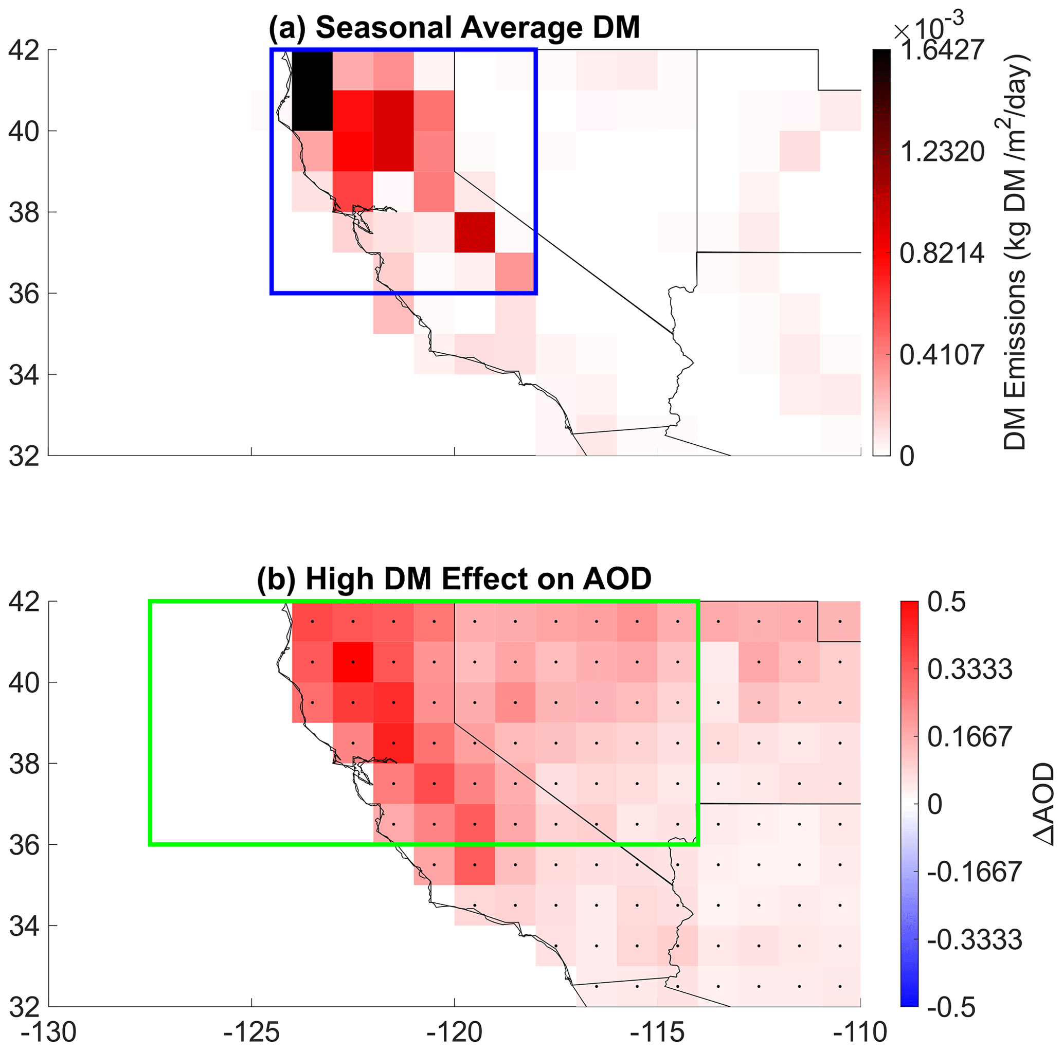
Figure 1Distribution of fires and the corresponding aerosol optical depth (AOD) anomaly impacts during the fire season. (a) 2003–2022 average daily fire dry matter (DM) emissions for the southwestern United States during the fire season (June–October). Blue box signifies the nCA (northern California) region, where average daily fire emissions are the highest. (b) 2003–2022 June–October daily MODIS Aerosol optical depth (AOD) difference between average AOD on 90th percentile DM (DM90) and average AOD on 10th percentile DM (DM10) days during the 2003–2022 June–October period. ΔAOD represents AOD(DM90) − AOD(DM10). Green box symbolizes the nCA-NV (northern California–Nevada) region, where increases in AOD and changes in cloud properties (Fig. 11) are most significant. Black dots represent statistically significant differences at 90 % confidence according to a two-tailed test.
It should be noted that while this method allows for the comparison of meteorology during very similar weather conditions, it does not completely remove the possibility of random meteorological fluctuations within the stratification that can affect the anomalies. Therefore, if anomalies are found, causality is difficult to discern.
3.3 Regions of interest
First, the region within the southwestern US in which the most significant fire emissions originate was discerned. Based on what is generally considered to be the time of year in which most wildfires occur in the western US (Urbanski, 2013; Urbanski et al., 2011), data were collected from 1 June to 31 October for the period 2003–2022. The period 2003–2022 was chosen as this is the time period in which Aqua satellite data are available for the fire season. Analysis was limited to fire seasons as opposed to the entire year so that the threshold for what constitutes a 90th percentile fire is increased. First, for each grid cell, the 2003–2022 seasonal average daily DM emission was taken. The portion of the southwestern US that had the largest 2003–2022 seasonal average daily DM emissions is the region that is referred to as “northern California” (nCA), which is highlighted in the blue box in Fig. 1a. The reason for limiting DM data to this region is again to ensure that the threshold for 90th percentile DM is kept high. The nCA region is characterized by temperate forests along the coastline in the far north and in the east. Agricultural lands are scattered throughout almost every grid cell in nCA, with higher concentrations in the central valley and the coastal north. Grasslands are also found throughout most grid cells in this region, with higher concentrations in central CA. The dominant contributor of DM in this region is the temperate forests in the north (Fig. S3). At this time of year, predominant wind patterns in nCA would favor transportation of smoke from these fires to northern Nevada. During the fire season, northwesterlies tend to blow across nCA towards northern Nevada, and south westerlies blow through the central valley and Sierra Nevada (Zaremba and Carroll, 1999; LeNoir et al., 1999). Therefore, the expectation is for the majority of wildfire aerosols to be concentrated in nCA and neighboring northern and central Nevada. In differentiating AOD anomalies on high nCA DM days and AOD anomalies on low nCA DM days, AOD is found to be anomalously positive in both nCA and Nevada (Fig. 1b), confirming this hypothesis. However, there are also significant AOD anomalies throughout the entire region. For reasons that will be explained in Sect. 4.1, the main analysis will still be concentrated on northern CA and Nevada. From this point forward, the focus will be on the effects of the fires in the blue box in Fig. 1a (nCA) on the area highlighted in the green box (nCA-NV) in Fig. 1b.
3.4 Heating rate
The aerosol shortwave heating rate of the atmosphere, SWHaer, was calculated using
where t is time in days, g is gravity, cp is the heat capacity at constant pressure, Faer is the shortwave radiative effect of the aerosols, and p is pressure. Faer itself was derived from the CERES SYN1deg-Day downward and upward shortwave radiative fluxes. Faer between two atmospheric layers is given by
where SWd1 denotes downward shortwave flux at the higher layer, SWu1 denotes upward shortwave flux at the higher layer, SWd2 denotes downward shortwave flux at the lower layer, and SWu2 denotes upward shortwave flux at the lower layer.
4.1 High and low surface relative humidity stratification
The fingerprints of a traditionally defined semi-direct effect where aerosols coincide with clouds would entail an anomalous warming of the cloud layer and a corresponding decrease in RH. However, the meteorological conditions around which fires tend to occur need to be considered. As previously stated, large fires tend to occur during fire weather, which includes hot, dry, and windy conditions (Varga et al., 2022). Hot and dry conditions themselves are associated with high-pressure anomalies in this region (Fig. S4). Therefore, these fire weather conditions need to be “filtered out” as much as possible to isolate any potential semi-direct effects. Therefore, in addition to DM, variables need to be stratified by a second variable to account for the influence of meteorology on P, CF, and cloud properties. Fire season data were stratified by high (75th percentile) vs. low (25th percentile) Ts, RHs, Us, and surface pressure to determine which variable was associated with the largest DM and successfully filtered out fire weather condition anomalies. The 75th and 25th percentiles were chosen for the potential second stratification variables as opposed to extremes (90th and 10th percentiles) so as to ensure a robust number of data points and to have a dataset that is more representative of common conditions in the region. Figure 2 depicts CDFs for meteorological conditions and DM under high RHs extremes (RHs75) and low RHs extremes (RHs25) in the entire southwestern US. RHs was chosen as the second stratification variable, as stratifying nCA DM by high (RHs75) and low RHs conditions (RHs25) and differentiating the means of these distributions yields a significant DM anomaly of kg m−2 d−1. The absolute value of this anomaly is an order of magnitude higher than the differences in mean DM between high and low conditions of the other potential stratification variables (surface pressure, Ts, and Us) (Figs. S4, S5, and S6). This indicates that fire occurrence and/or fire emissions are more dependent on RHs than these other fire weather variables. Low RHs extremes in the southwestern US are associated with significantly higher T throughout the troposphere and surface, significantly reduced RH throughout the troposphere and surface, and significantly lower CF, while high RHs extremes are associated with the opposite (Fig. 2). This demonstrates a need to separate the effects of fires from the meteorological effects of low RHs extremes, as positive DM anomalies are significantly more likely to occur on (RHs25) days as opposed to (RHs75) days, which is expected, as moisture and moist plants suppress the ability of fires to grow and be maintained (Minnich and Chou, 1997; Ford and Johnson, 2006). The immediate direct effect of BB aerosols tends to be a net cooling of the surface (Sakaeda et al., 2011; Abel et al., 2005). However, certain semi-direct effects, such as the burning off of low clouds, may overpower this effect, leading to a net surface warming. As the meteorological conditions associated with low RHs days are also hallmarks of a semi-direct effect (Fig. 2), from here onward data will be stratified into four categories: one with high DM and high RHs (DM90, RHs75), one with low DM and high RHs (DM10, RHs75), one with high DM and low RHs (DM90, RHs25), and one with one with low DM and low RHs (DM10, RHs25). In differentiating the average of the variables on (DM90, RHs75) days and (DM10, RHs75) days, the effects of the meteorological conditions that come with high DM extremes can be minimized. However, a caveat to this analysis is that it is possible there may be a bias towards lower values of RHs in the DM90 datasets compared with the DM10 datasets, as fire weather conditions can invigorate fire activity. Therefore, while this analysis removes a lot of weather variability as per Fig. 2, it does not remove all of it and caution should be taken when interpreting the results. Figure 3 demonstrates that during large fires, AOD anomalies under both high and low RHs stratifications are significantly positive in the nCA-NV region. The increase in mean AOD is larger under low RHs at 0.24 ± 0.04. The corresponding change under high RHs is 0.13 ± 0.05. As the AOD is consistently significant only in the nCA-NV region under both stratifications, this region will be the focus of the study.
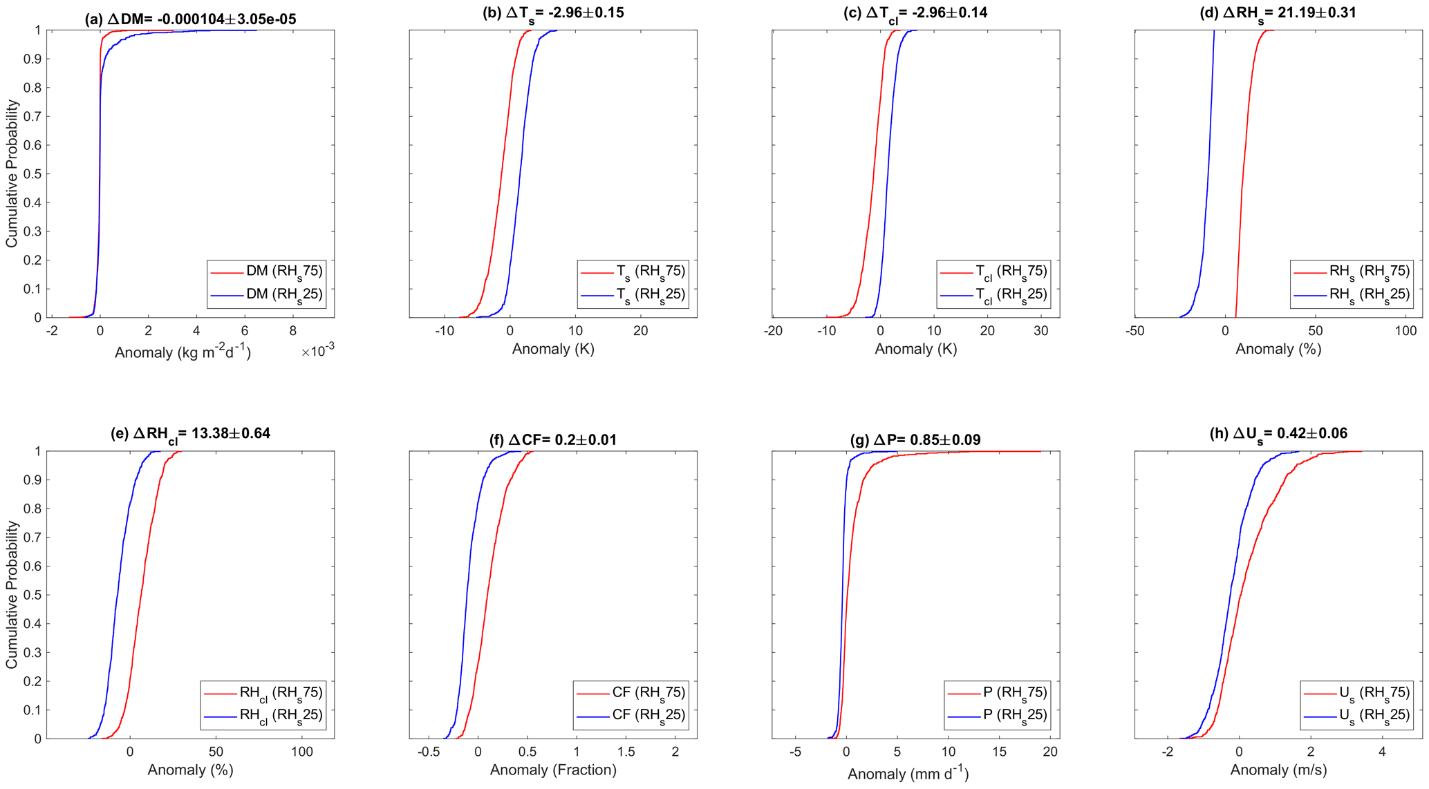
Figure 2Dependence of meteorological variables on high versus low surface relative humidity (RHs) during the fire season. Regional average cumulative distribution functions (CDFs) for variable anomalies stratified by 75th percentile surface relative humidity (RHs75) days (red) and 25th percentile (RHs25) days (blue) during the 2003–2022 June–October period. Variables depicted include (a) northern California (nCA) fire dry matter (DM) emissions, (b) southwestern US surface temperature Ts, (c) nCA-NV cloud layer (850–300 hPa) average temperature TCL, (d) southwestern US surface relative humidity RHs, (e) southwestern US cloud layer average relative humidity RHCL, (f) southwestern US cloud fraction CF, (g) southwestern US precipitation P, and (h) southwestern US surface wind speed U. Δ represents the difference between the variable's average anomaly for RHs75 and RHs25 days.
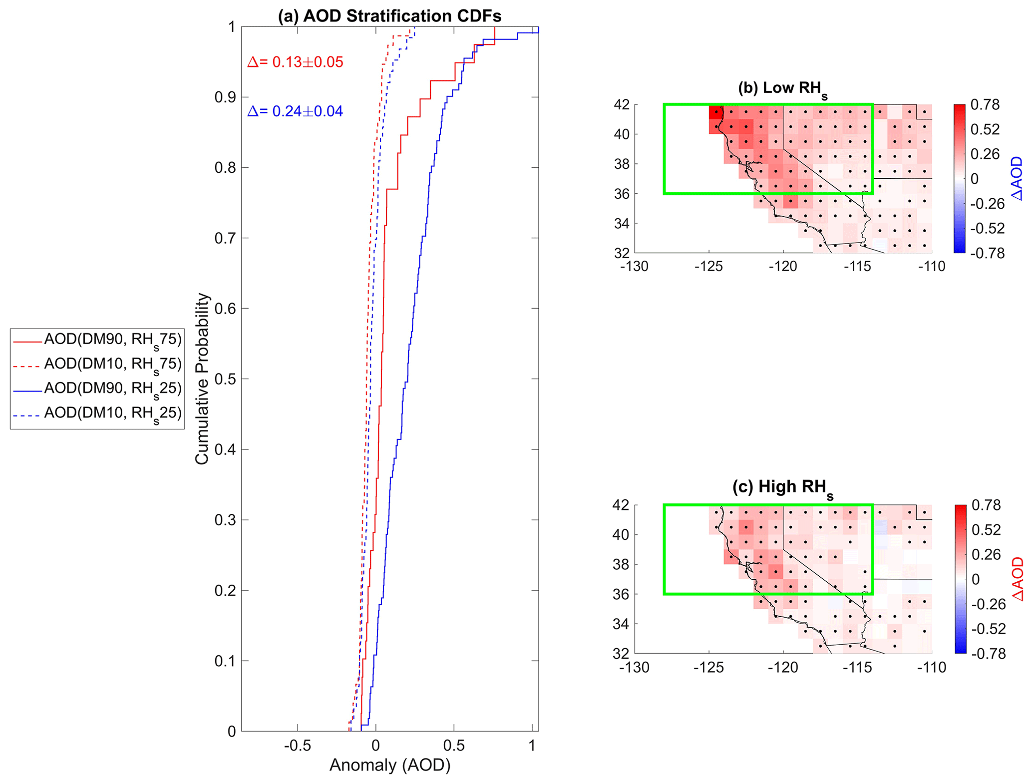
Figure 3Difference in AOD anomalies on high and low RHs days during the fire season. Daily northern California–Nevada (nCA-NV) AOD anomalies stratified by nCA-NV RHs and nCA DM extremes during the 2003–2022 June–October period. Panel (a) displays cumulative distribution functions for daily June–October 2003–2022 daily nCA-NV AOD stratified by high (90th percentile) nCA DM emissions and high nCA-NV RHs AOD(DM90, RHs75) (solid red line), low (10th percentile) DM and high RHs AOD(DM10, RHs75) (dashed red), simultaneously high DM and low RHs AOD(DM90, RHs25) (solid blue line), and simultaneously low nCA DM and low RHs AOD(DM10, RHs25) (dashed blue line). The red ΔAOD represents the difference between the solid red and dashed red line AOD(DM90, RHs75)−AOD(DM10, RHs75) and the blue ΔAOD represents the difference between the solid and dashed blue lines AOD(DM90, RHs25)−AOD(DM10, RHs25). Panel (b) depicts a map of AOD(DM90, RHs25)−AOD(DM10, RHs25). Pearson cross-correlation coefficient r between ΔAOD and nCA DM emissions is depicted in the top left corner. Panel(c) depicts a map of average AOD(DM90, RHs75)−AOD(DM10, RHs75). Black dots in panels (b) and (c) represent statistically significant differences at the 90 % confidence interval according to a two-tailed test.
4.2 Vertical distribution of black carbon and absorption in nCA-NV region
Freshly emitted BC is highly hydrophobic, and as it ages it becomes less resistant to accumulating water droplets (Lohmann et al., 2020). BC has an average lifetime of 1 week (Lohmann et al., 2020), and the aging process begins after 1–2 d (He et al., 2016). Furthermore, in a region with such low fire season wet deposition such as the southwest US, the BC on average can live much longer than 1 week (Ogren and Charlson, 1983). Therefore, hydrophobic and hydrophilic BC profiles are important to differentiate because they can give an idea of how long the BC stays in the atmosphere and it hints at how much BC can contribute to indirect and semi-direct effects. Figure 4 displays high compared with low DM mass mixing ratio anomalies for BCphi, BCpho, and combined BC on high and low RHs days. Significant positive anomalies of BC mass mixing ratio are present from 950 to 300 hPa for all types of BC under both (DM90, RHs75) and (DM90, RHs25) conditions compared with the corresponding low fire conditions. The most significant increase in BC is from about 950 to 600 hPa for the (DM90, RHs75) days, and from 950 to 550 hPa for the (DM90, RHs25) days. Comparing the MERRA-2 BC profiles with the CALIPSO DM90–DM10 months during 2006–2021 smoke aerosol daytime and nighttime extinction coefficient profile, MERRA-2 places more absorbing aerosols below 700 hPa, while CALIPSO generally places more absorbing aerosols above 700 hPa (Fig. S7). Therefore, it is important to note that CALIPSO profiles do not agree with MERRA-2 when it comes to the positioning of the smoke in the troposphere. However, as the MERRA-2 and CALIPSO profiles are not temporally consistent, the comparison between these profiles is not 1−1. Additionally, as the CALIPSO profiles are not temporally consistent with the rest of the data in this paper, their use is not preferred over the MERRA-2 profiles.
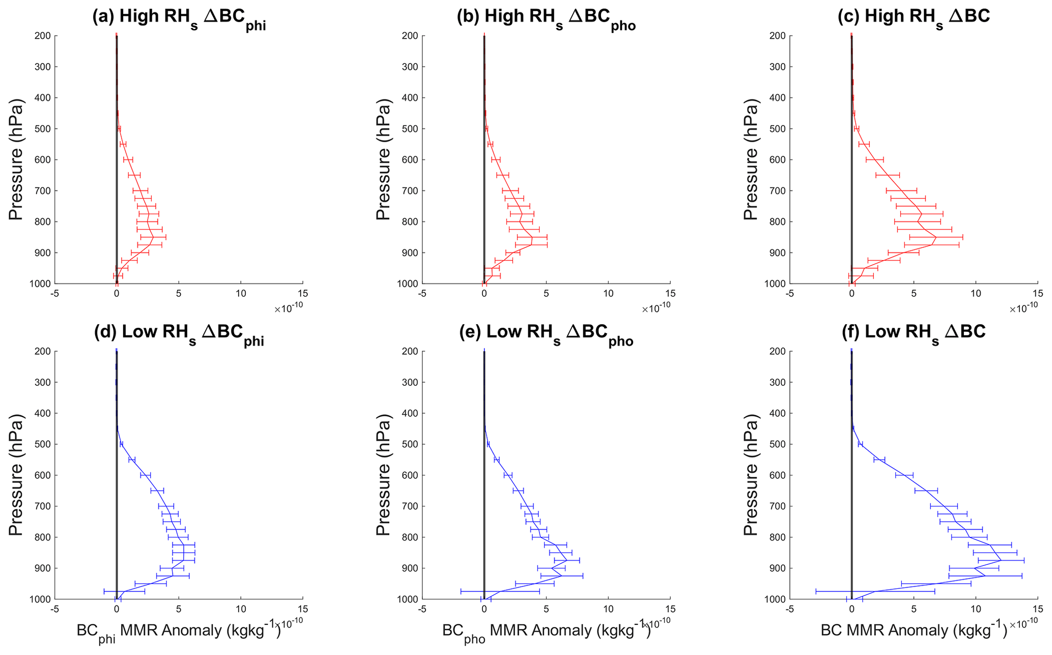
Figure 4Difference in MERRA-2 black carbon (BC) profiles on high vs. low fire days stratified by differing RHs conditions in the nCA-NV region during the 2003–2022 June–October period. Profiles of both aged hydrophilic black carbon BCphi (a, d) as well as freshly emitted hydrophobic black carbon BCpho (b, e) are depicted in addition to total BC (c, f). All types of BC have significant anomalies from 850 to 300 hPa under both high RHs (a–c) and low RHs conditions (d–f).
There is roughly an equal amount of BCphi and BCpho during both high and low RHs days, indicating that on these days there is roughly as much fresh as aged aerosol in the troposphere. This is important, as the quantity of BCpho indicates that microphysical effects are possible, since it suggests a large amount of CCN are present in the troposphere. Additionally, the presence of aged BC indicates that the BC can affect the atmosphere radiatively over the course of multiple days. To estimate the impact of these aerosols on the troposphere over time, an SWHaer profile was created from CERES radiative flux data (Fig. 5). Shortwave profiles used to generate these heating rate profiles, along with LW profiles, are shown in Fig. S8. Under both (DM90, RHs75) (Fig. 5a) and (DM90, RHs25) (Fig. 5b) RHs conditions compared with the corresponding low DM conditions, there is a positive SWHaer anomaly from 850 hPa to the next highest pressure level in the CERES dataset, 500 hPa. For high RHs, this corresponds to a heating rate of SWHaer= 0.041 ± 0.016 K d−1, and for low RHs, this corresponds to a heating rate of SWHaer= 0.093 ± 0.019 K d−1. Spatially, the 850–500 hPa heating rate is significant over almost all grid cells in the region of interest where there are data, with the most positive heating rates over eastern nCA and eastern Nevada (Fig. 5c, d).
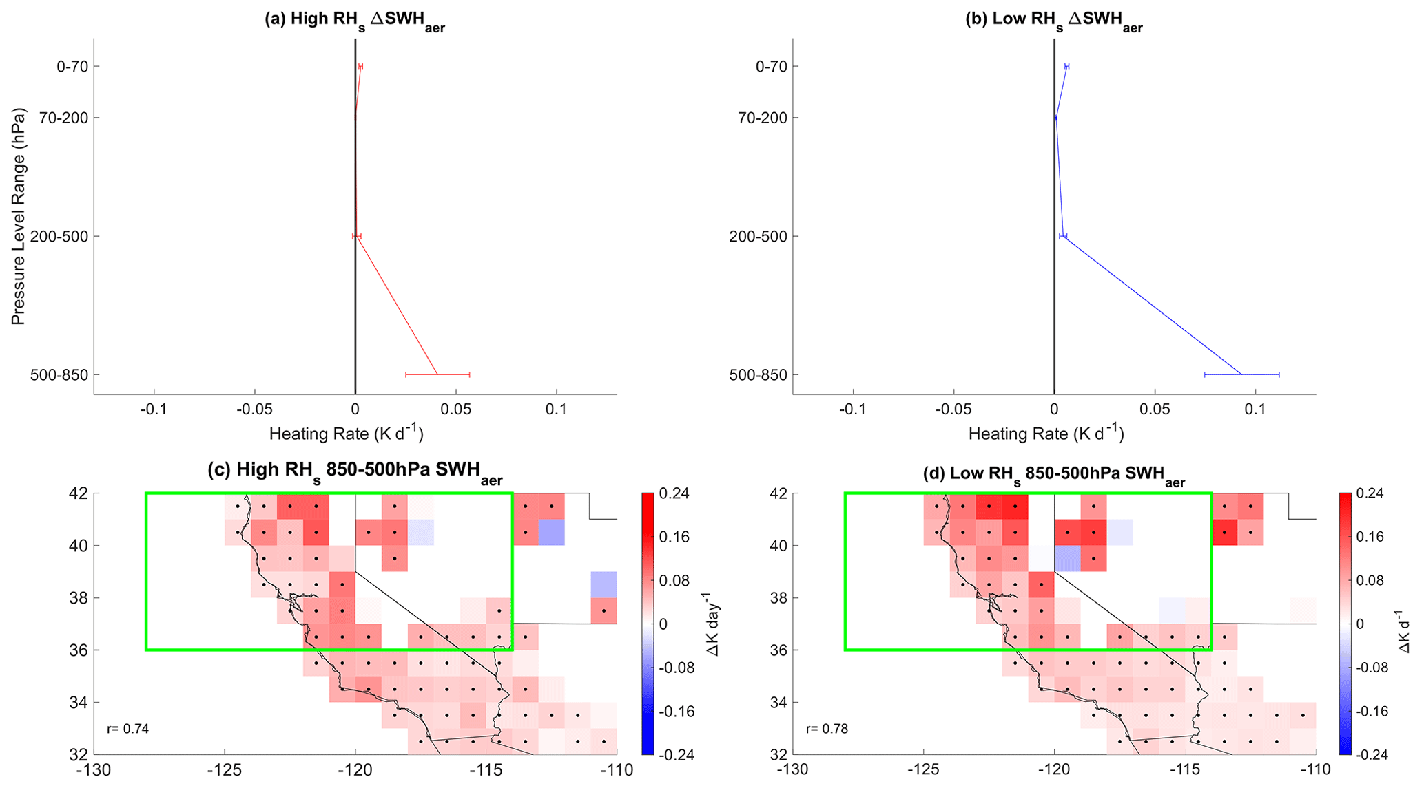
Figure 5High minus low DM days regional average aerosol-only shortwave heating rate SWHaer profiles under differing RHs conditions during the 2003–2022 June–October period. There is a significant shortwave aerosol heating rate from 850 to 500 hPa under both high RHs (a) and low RHs conditions (b). Also depicted are spatial maps for high minus low fire days (c) under simultaneously high RHs conditions and (d) under simultaneously low RHs conditions. Black dots represent statistical significance at the 90 % confidence interval. r represents the cross correlation between SWHaer and AOD.
It should be noted that aerosol absorption can be affected by water vapor in the atmosphere, which can cause swelling and lensing effects that increase absorption (Wu et al., 2018; Peng et al., 2016). Therefore, this possibility will be investigated in Sect. 4.3.
4.3 Responses in temperature, humidity, and cloud profiles
Figure 6 displays the 2003–2022 June–October nCA-NV vertical profiles of high minus low fire T (Fig. 6a, e) and RH (Fig. 6c, g) profiles. Figure 6a–d are stratified by high RHs, while Fig. 6e–h are stratified by low RHs. In both Fig. 6a and e, the temperature anomalies in the 850–300 hPa pressure level range are consistently significant and positive at around 1 K. Comparing Fig. 6 with Fig. 4, the positive differences in temperature anomaly are generally consistent with the positive BC anomalies. Also, the changes in T from 850 to 500 hPa are spatially consistent with the 850–500 hPa heating rate anomalies where data are available (Fig. 5c, d). Under both high RHs (Fig. 6c) and low RHs (Fig. 6g) conditions, RH anomalies throughout the entire profiles are negative but are only consistently significant during high RHs extremes. The AIRS CF profile under high RHs conditions (Fig. 6d) demonstrates significant negative anomalies from 300 to 600 hPa that are consistent with significant negative RH anomalies and significant positive T anomalies. However, there is an increase in CF at 850 hPa (Fig. 6d). This pressure level corresponds to the highest concentration of BCphi (Fig. 4c), and perhaps this indicates there is cloud seeding occurring at this pressure level. For the low RHs profile, there is only a significant negative cloud anomaly close to the surface at 925 hPa (Fig. 6h).
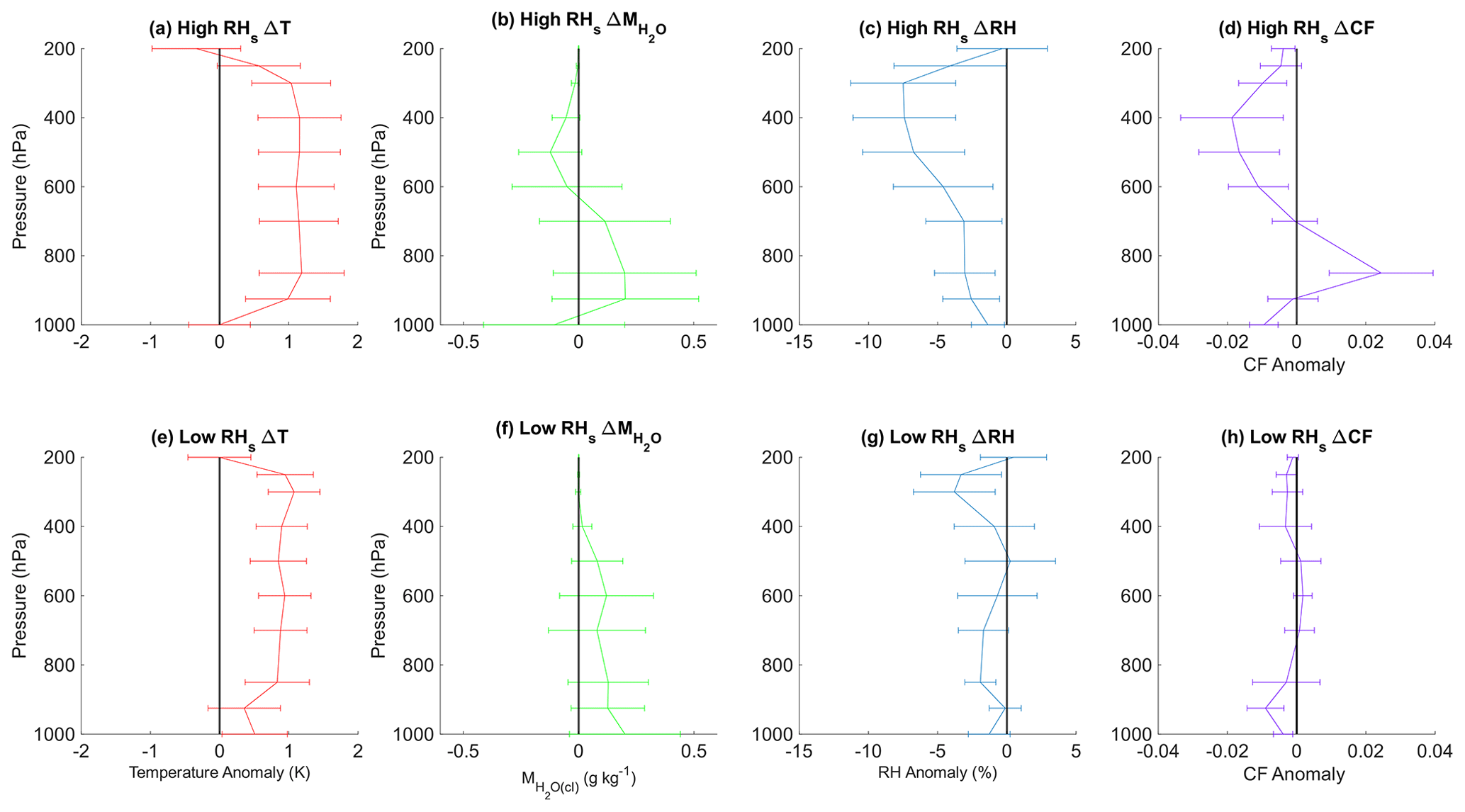
Figure 6Responses in AIRS temperature T, water mass mixing ratio , relative humidity RH, and cloud fraction CF profiles to large fires under high and low RHs extremes during the fire season. nCA-NV regional temporal average differences in T, water mass mixing ratio , and relative humidity RH profiles for high minus low DM conditions stratified by RHs75 (a–d) and RHs25 (e–h) during the 2002–2023 fire season (June–October). Error bars represent the 90 % confidence interval.
Aside from temperature, the other potential factor that could affect RH is that of specific humidity, which is analogous to the water mass mixing ratio . Figure 6b and f depict the effect of fires on anomalies under high RHs and low RHs conditions, respectively. There is no significant anomaly under high or low RHs conditions, but it is consistently positive at 700 hPa and below. Furthermore, the changes in the RH profile follow the changes in the T profile as opposed to the profile, implying the positive T anomalies generally dominate the change in RH anomalies. The insignificant change in also casts doubt that water vapor is affecting the absorption of the aerosols in any significant way.
While these profiles provide a general overview of how T, , RH, and CF are changing over the region of interest, it is important to determine whether these changes are consistent spatially with one another as well as whether the changes coincide with BC anomalies. As the T, RH, and CF anomalies are strongest during high RHs days, the focus from here will be on the meteorological effects of high DM on high RHs days. Figures 7–11 depict the effect of fires on the spatial distributions of BC, T, , RH, and CF anomalies at each AIRS pressure level up to 200 hPa under high RHs conditions. The positive MERRA-2 BC anomalies in Fig. 7 correlate positively and significantly with MODIS AOD for each pressure level between 925 and 300 hPa (Fig. 7b–h), and are spatially consistent with positive AIRS T anomalies (Fig. 8). Shifting attention to Fig. 9, there appear to be significant negative anomalies in in northeastern Nevada from 700 to 400 hPa and significant positive anomalies over grid cells associated with large fires (Fig. 1a) in the lower troposphere (925–850 hPa). Comparing these changes in T and spatially with changes in RH (Fig. 10), it appears that changes in T tend to dominate changes in RH over CA, western NV, and southern NV, while changes in appear to contribute to the negative RH anomaly in northeastern NV. Additionally, the positive at 850 hPa appears to mitigate the negative RH anomalies at the same level, which may explain why BC appears to be able to act as a CCN at this level but not others: RH does not decrease enough to prevent clouds from forming. The increase in has a myriad of possible explanations. It may be due to the emission of moisture from the burned vegetation (Jacobson, 2014; Dickinson et al., 2021), from lofting of water vapor from the surface to higher levels of the atmosphere (Yu et al., 2024), or from moisture advection due to a change in wind vectors from the northeastern part of Nevada towards California (Fig. S9). This scattered significant increase in , being relegated to a few grid cells in a few pressure levels, is not generally spatially consistent with the changes in SWHaer (Fig. 5c), especially compared with the spatial distribution of BC (Fig. 7), further indicating that lensing effects are not the dominant contributor to the increase in aerosol absorption. Viewing Fig. 11c, the increase in CF at 850 hPa appears to be driven predominantly by a few significant and large coastal CF anomalies. This indicates that there is an increase in shallow marine clouds at this pressure level, while clouds at other pressure levels are generally being suppressed. Figure 11 demonstrates that significant negative CF anomalies are generally spatially consistent with negative RH anomalies from 700 to 400 hPa. The significant negative CF anomalies in northeastern Nevada that correspond to significant negative RH anomalies, but not significant positive T anomalies, at 700 hPa and higher indicate that the difference in clouds in this region is dependent on specific humidity. This may be due to a transport of moisture outside of these grid cells due to anomalously positive southeastern wind speed anomalies in some of these grid cells (Fig. S9b) that advect moisture towards southern California and southern Nevada; however, further scrutiny is warranted to confirm this. It is not known if these wind speed anomalies are related to T anomalies to the west or if these wind speed anomalies in this region are an artifact. Changes in wind vectors are further analyzed in Sect. S3. As the change in T is the more robust signal over all parts of the troposphere, the changes in T will be the focus of the remainder of the paper.
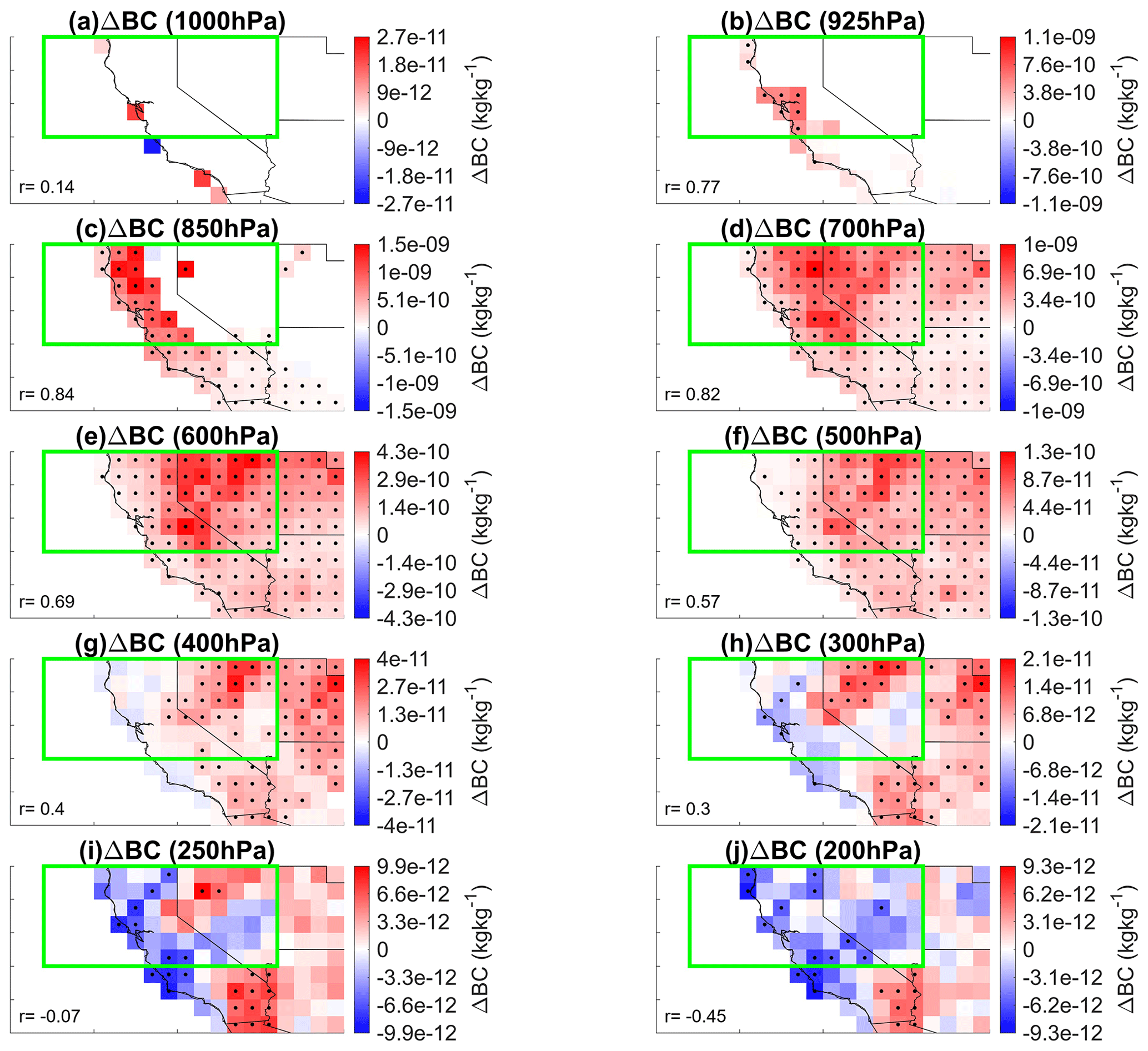
Figure 7High minus low DM days MERRA-2 BC anomalies at all AIRS pressure levels from 1000 to 200 hPa (a–j) under high RHs conditions during the 2003–2022 June–October period. Black dots indicate statistical significance at the 90 % confidence interval. r values indicate spatial Pearson cross correlations between total BC and MODIS AOD.
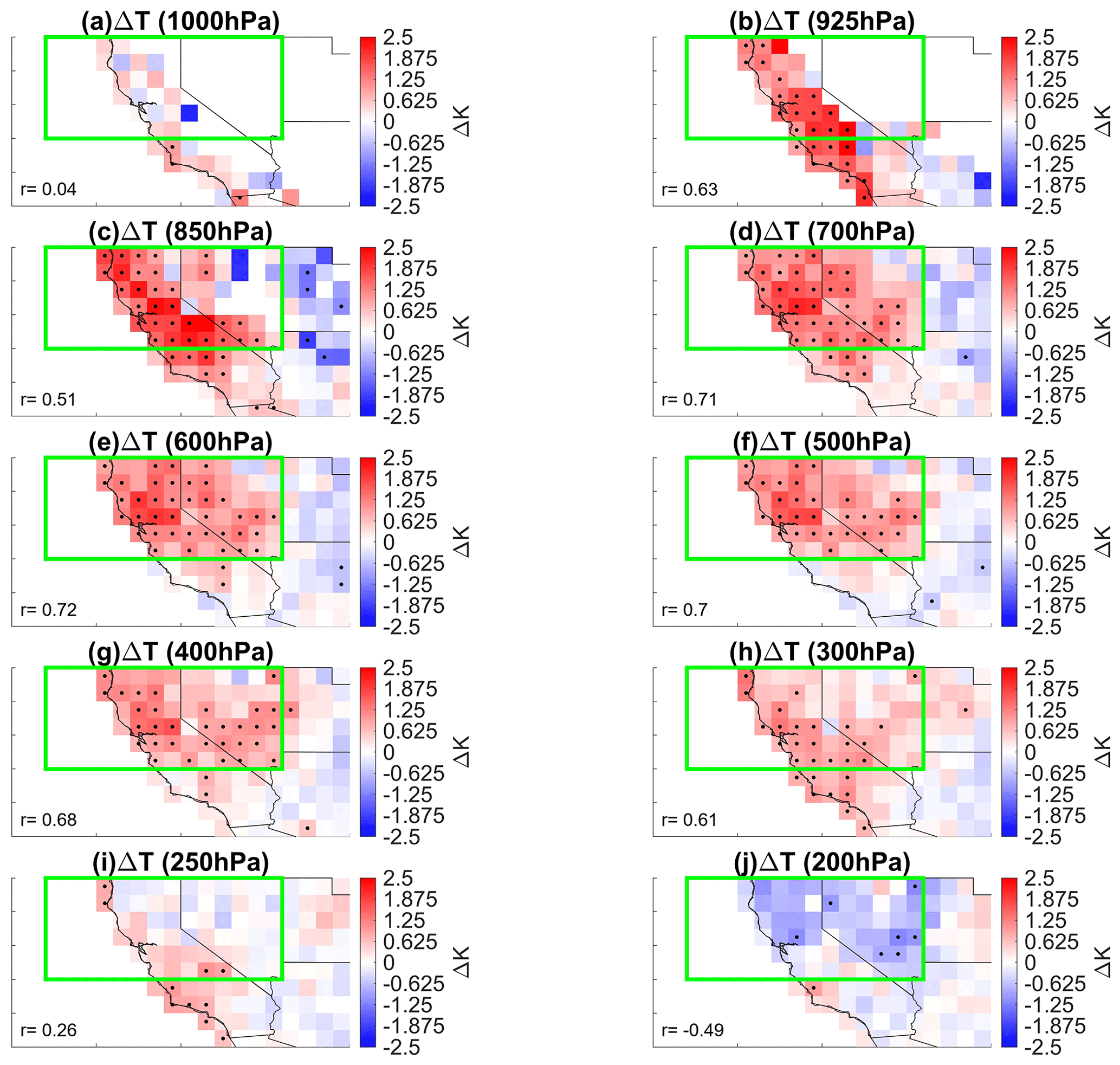
Figure 8High minus low DM days AIRS T anomalies at all AIRS pressure levels from 1000 to 200 hPa (a–j) under high RHs conditions during the 2003–2022 June–October period. Black dots indicate statistical significance at the 90 % confidence interval. r values indicate spatial Pearson cross correlations between T and MODIS AOD.
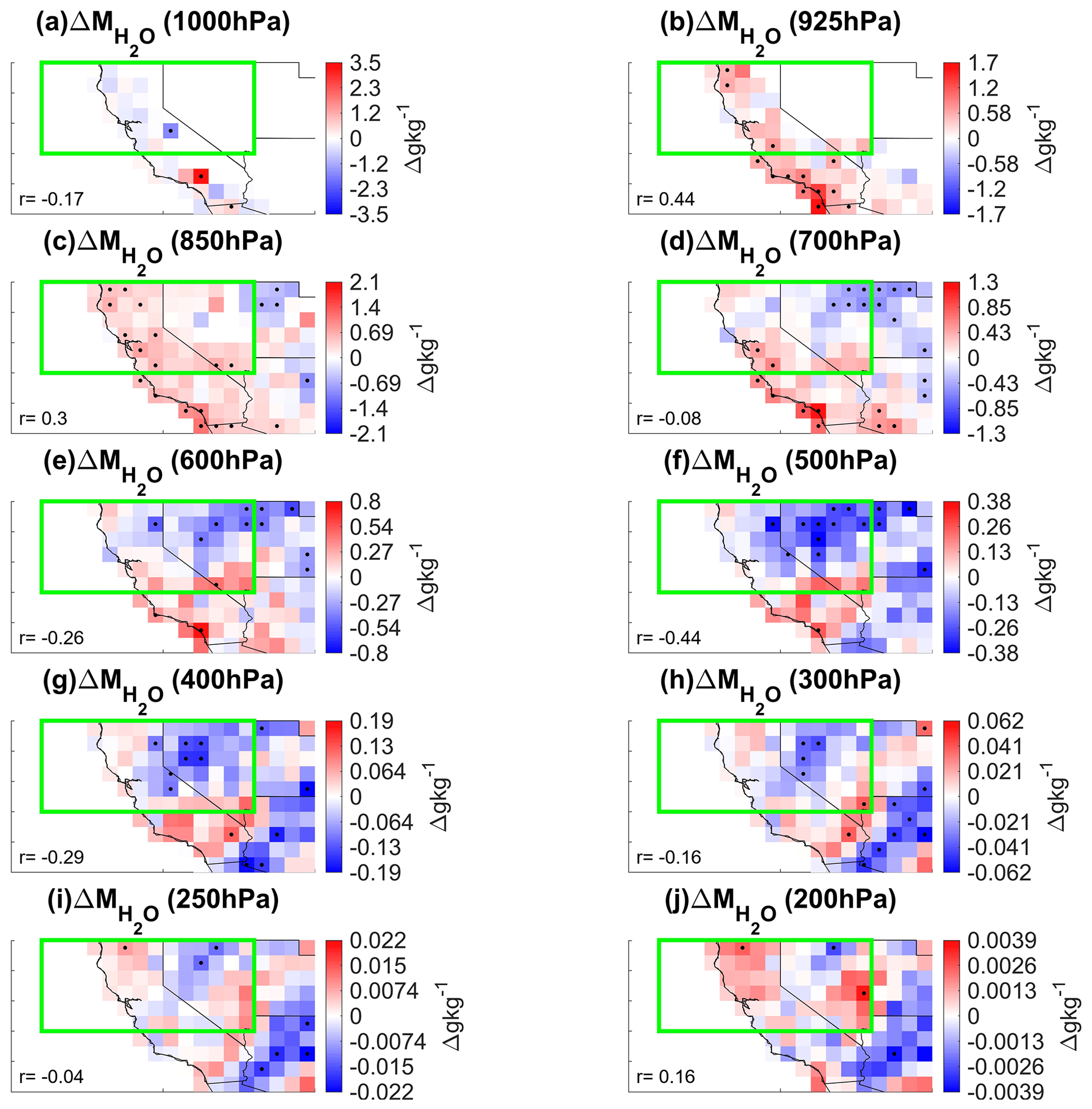
Figure 9High minus low DM days AIRS anomalies at all AIRS pressure levels from 1000 to 200 hPa (a–j) under high RHs conditions during the 2003–2022 June–October period. Black dots indicate statistical significance at the 90 % confidence interval. r values indicate spatial Pearson cross correlations between total and MODIS AOD.
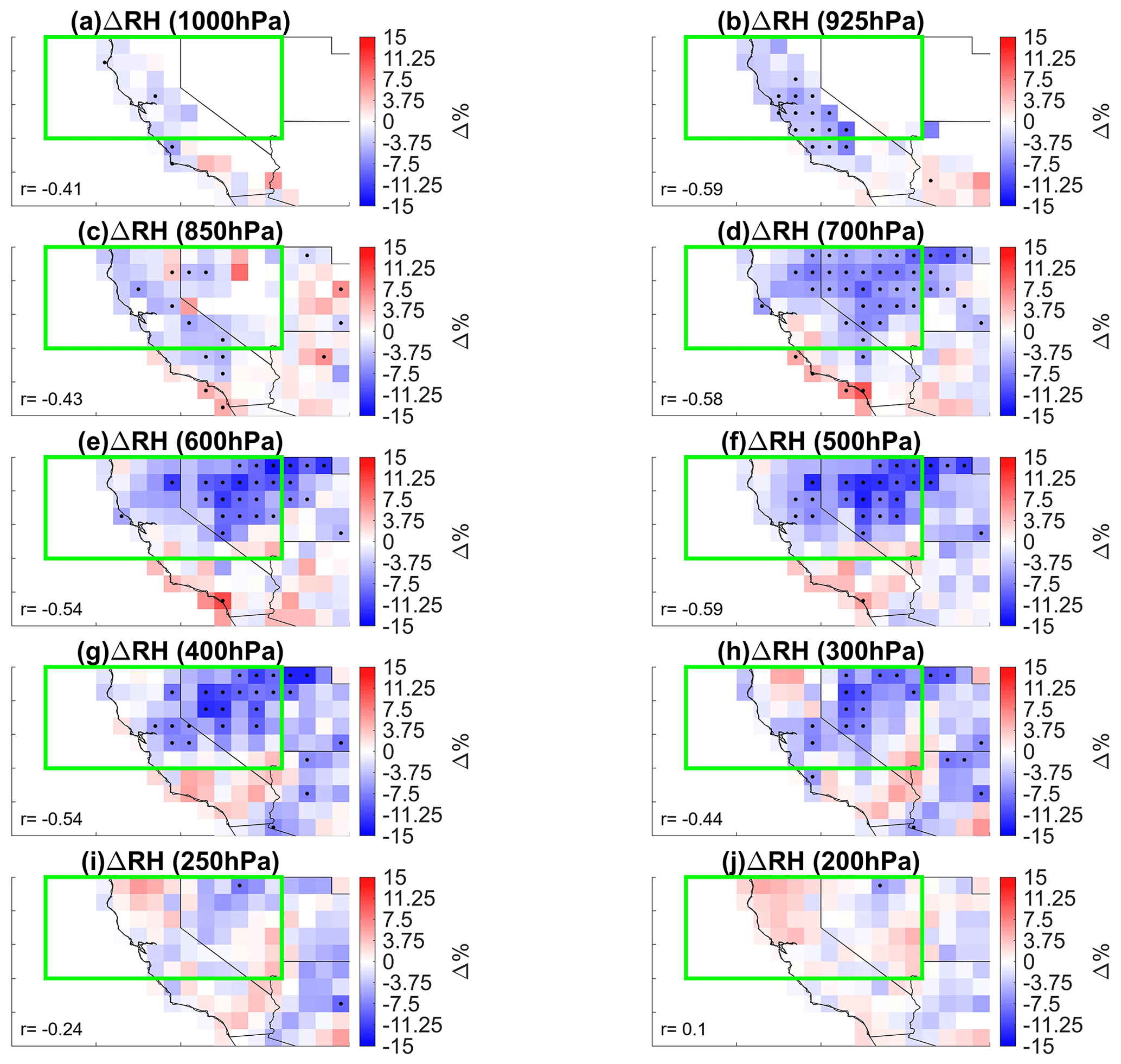
Figure 10High minus low DM days AIRS RH anomalies at all AIRS pressure levels from 1000 to 200 hPa (a–j) under high RHs conditions during the 2003–2022 June–October period. Black dots indicate statistical significance at the 90 % confidence interval. r values indicate spatial Pearson cross correlations between RH and MODIS AOD.
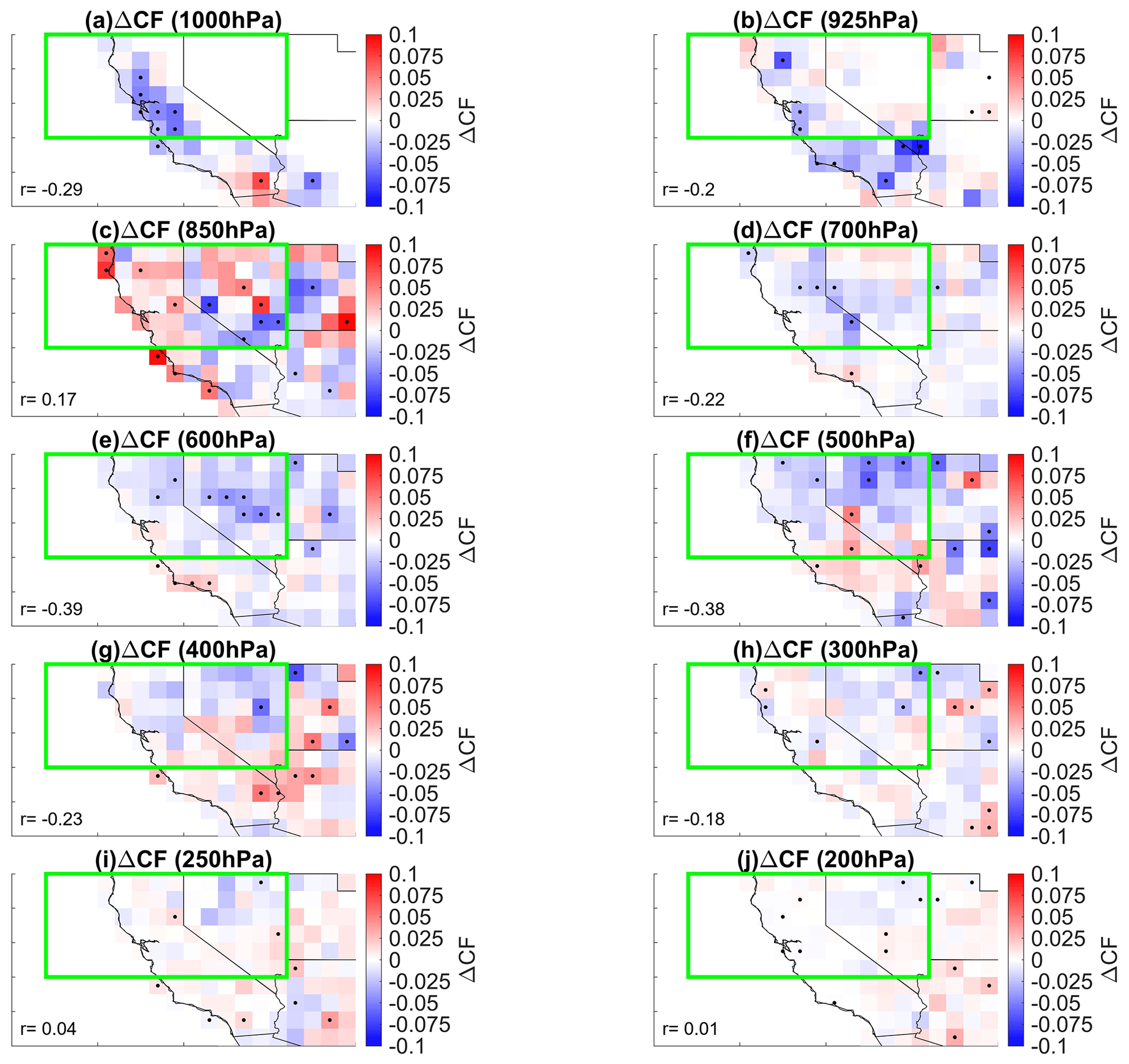
Figure 11High minus low DM days AIRS CF anomalies at all AIRS pressure levels from 1000 to 200 hPa (a–j) under high RHs conditions during the 2003–2022 June–October period. Black dots indicate statistical significance at the 90 % confidence interval. r values indicate spatial Pearson cross correlations between CF and MODIS AOD.
4.4 Changes in cloud type, precipitation, and shortwave flux
With AIRS data indicating that large fires are associated with enhanced T, as well as lower RH and CF, it is essential to determine how liquid vs. ice clouds are impacted and what the corresponding impacts on P and radiative balance are. Figure 12 displays CDFs for nCA-NV regional average variable anomalies during simultaneously high DM and low RHs days (solid red), simultaneously low DM and high RHs days (dashed red), simultaneously high DM and low RHs days (solid blue), and simultaneously low DM and low RHs days (dashed blue). Figure 12a and b demonstrate that during high RHs extreme days, the effect of fires on the liquid water cloud fraction CFlw distribution and cirrus cloud fraction CFcir distribution is a significant shift towards a preference for negative anomalies. The effect of the large fires creates an average −0.04 ± 0.02 CFlw anomaly and an average −0.05 ± 0.04 CFcir anomaly under high RHs conditions. In addition, MODIS total CF shifts by −0.07 ± 0.05 under the same stratifications. Precipitation also shifts significantly by −0.3 ± 0.23 mm d−1. However, these shifts are significant only for high RHs extreme days (Fig. 12). The explanation of why the distribution shifts farther towards negative anomalies when anomalously large fires occur during high RHs compared with low RHs extremes lies in Fig. 2. During low RHs days, RH throughout the troposphere is already significantly lower than normal conditions (Fig. 2e), as temperatures throughout the troposphere are already high (Fig. 2c) and atmospheric water vapor content is low. This creates conditions of negative CF anomalies (Fig. 2f). Therefore, further increasing the already high T should not lead to significantly lower cloud fraction, as RH is already low and clouds require 100 % RH to form. This can also be explained by the RH profile in Fig. 6g, which demonstrates through most parts of the troposphere that RH is not significantly lowered during fires. However, during simultaneously low DM and high RHs days, Fig. 12 demonstrates that conditions are favorable for clouds and rain. This is because during these high RHs extremes, T is lower and RH is high. Therefore, when anomalously large fires introduce a positive T anomaly, the drop in RH is significant enough to reduce the chances of seeing positive cloud and/or precipitation anomalies. In response to the higher probability of negative cloud fraction anomaly, the probability that SW radiation will be reflected into space decreases. This reduction in top-of-atmosphere shortwave flux leads to a net increase in cloud only (all-sky minus clear-sky) top-of-atmosphere radiative forcing TOAcld (Fig. 12f). Although it should be noted that this increase is not significant, it is significant and positive over much of the region marked by a decrease in CF (Fig. 13e, h), with a significant spatial cross correlation of r= −0.67. Regional all-sky SW and LW responses are shown in Fig. S10.
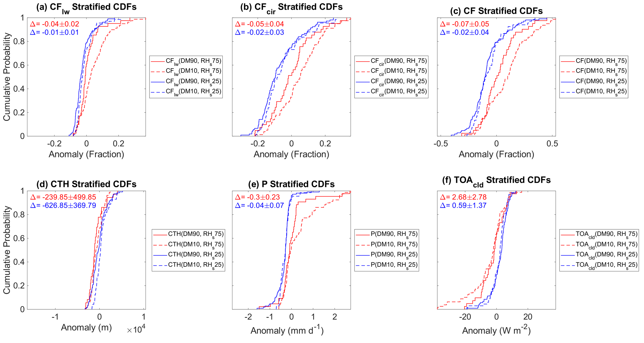
Figure 12Dependence of meteorological variables on high versus low RHs and fires during the fire season. Empirical CDFs for regional average daily anomalies of meteorological variables over the nCA-NV region during the 2003–2022 June–October period. Solid red line signifies variable anomalies are stratified by high nCA fire dry matter (DM) emissions and high nCA-NV RHs anomaly days (DM90, RHs75). The dashed red line signifies variable anomalies stratified by low DM and high RHs anomaly days (DM10, RHs75). The solid blue line represents variable anomalies stratified by high DM and low RHs anomaly days (DM90, RHs25). The dashed blue line symbolizes variable anomalies stratified by low DM and RHs anomaly days (DM10, RHs25). Variables depicted include (a) liquid water cloud fraction CFlw, (b) cirrus cloud fraction CFcir, (c) CF, (d) cloud top height CTH, (e) precipitation P, and cloud-only (all-sky minus clear-sky) net top-of-atmosphere flux TOAcld. The red Δ represents the differences in the mean of the solid red and dashed red lines (DM90, RHs75)−(DM10, RHs75). The blue Δ represents the differences in the mean of the solid blue and dashed blue lines (DM90, RHs25)−(DM10, RHs25).
Figure 13 displays composite differences between meteorological variables on simultaneously high DM and high RHs and simultaneously low DM and high RHs days for each grid cell over the entire southwestern US. Figure 13a and b display the composite differences in cloud layer (850 hPa 300 hPa) temperature TCL and cloud layer relative humidity RHCL. These plots depict that TCL significantly increases almost everywhere across California and Nevada, with the most significant increase in the green box (the nCA-NV region). The differences in TCL correlate significantly with differences in AOD at r= 0.72 across the entire southwestern US. The decreases in RHCL have a very similar spatial distribution to TCL, with the strongest decreases in the nCA-NV region. Again, this correlates significantly with AOD, with r= −0.55 over the entire southwest. The differences in all these variables across the southwestern US correlate significantly with AOD, supporting the assertion that aerosols concurrent with fires are associated with warming and drying. Of note are the changes in Ts and P, which are two variables intrinsically related to fire duration. Spatially correlating P with RHCL yields a significant, but notably weaker, correlation of r= 0.44, implying a relationship between the negative P anomalies and the biomass burning aerosols. However, it should be noted that although the regional P anomaly is significant and negative, it appears to be dominated only by strong changes in just a few grid cells. Ts correlates significantly with AOD over the southwestern US, with r= 0.51, and is generally spatially concurrent with increases in TCL with r= 0.72. The equivalent for Fig. 13 for low RHs days is given in Fig. S11. Of note for this supplementary figure is that there are weak, but significant and widespread, negative CF, RH, and P anomalies over nCA and eastern Nevada, despite not being significant in the regional average (Fig. 12c, e). This implies that the meteorological anomalies seen during high RHs days are also prevalent on low RHs days but weaker and less widespread due to the lower availability of moisture.
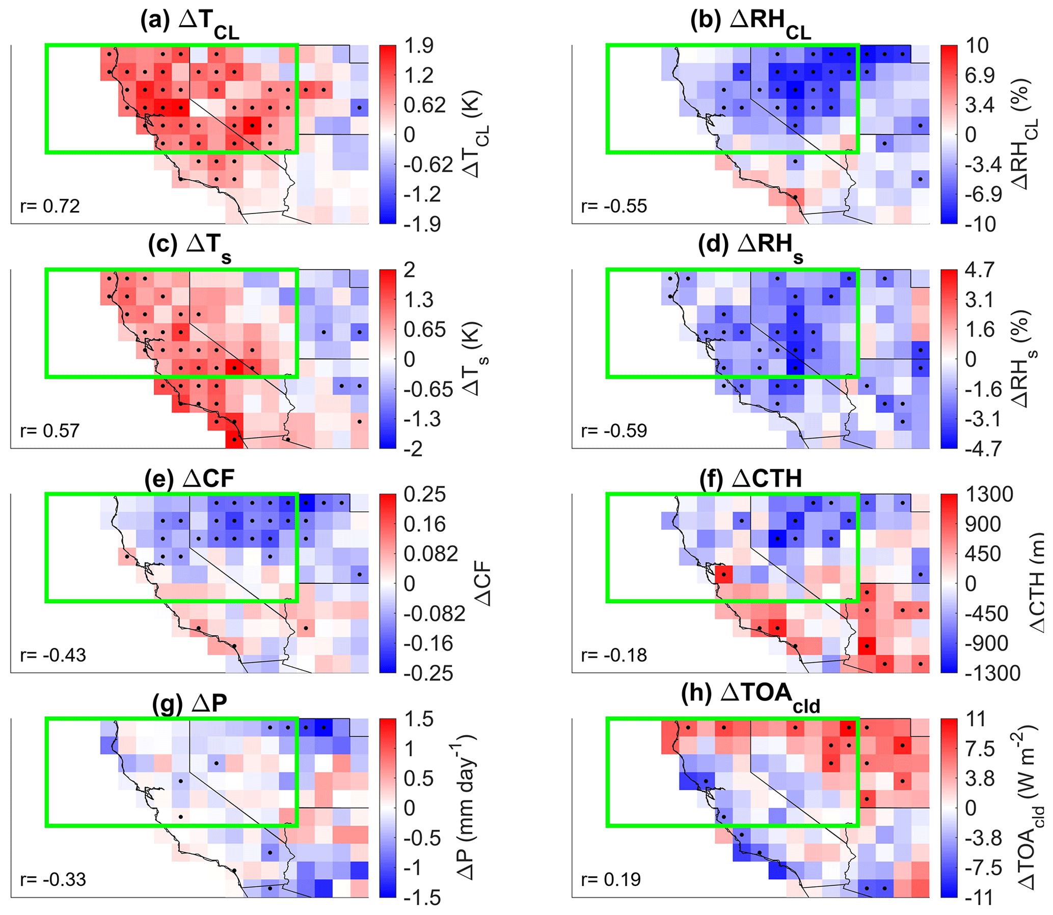
Figure 13Meteorological responses under high versus low nCA DM conditions with simultaneously high nCA-NV RHs during the fire season. Difference between average variable anomalies on high (90th percentile) nCA fire dry matter (DM) emission days and low (10th percentile) nCA DM emission days that occur on high nCA-NV RHs days during the 2003–2022 June–October period. Variables include (a) 850–300 hPa average temperature TCL, 850–300 hPa average relative humidity RHCL, (c) surface temperature Ts, (d) RHs, (e) CF, (f) CTH, (g) P, and (e) TOAcld. Black dots represent statistically significant differences at the 90 % confidence interval according to a two-tailed test. Pearson cross-correlation r values in each plot represent the spatial correlation between MODIS aerosol optical depth (AOD) anomaly and the variable anomaly depicted in the figure. All values of r are significant at the 90 % confidence interval according to a two-tailed test.
While cross correlations indicate that there is a statistically significant relationship between fires and meteorology, practical significance needs to be established as well. The effect sizes of high DM emissions on nCA-NV regional averages of the variables in Figs. 12 and 13 are depicted in Fig. 14. For high RHs extremes (Fig. 14a), the anomalously large fires are associated with a moderate to strong effect size on most of the relevant variables. Figure 14b demonstrates that during low RHs conditions, anomalously large fires are associated with a weak to no effect size on the relevant variables, aside from TCL in which fires have a very strong effect size. It should be noted that effect size does not imply causality but instead only quantifies how different the mean of a distribution is when a single variable is changed.
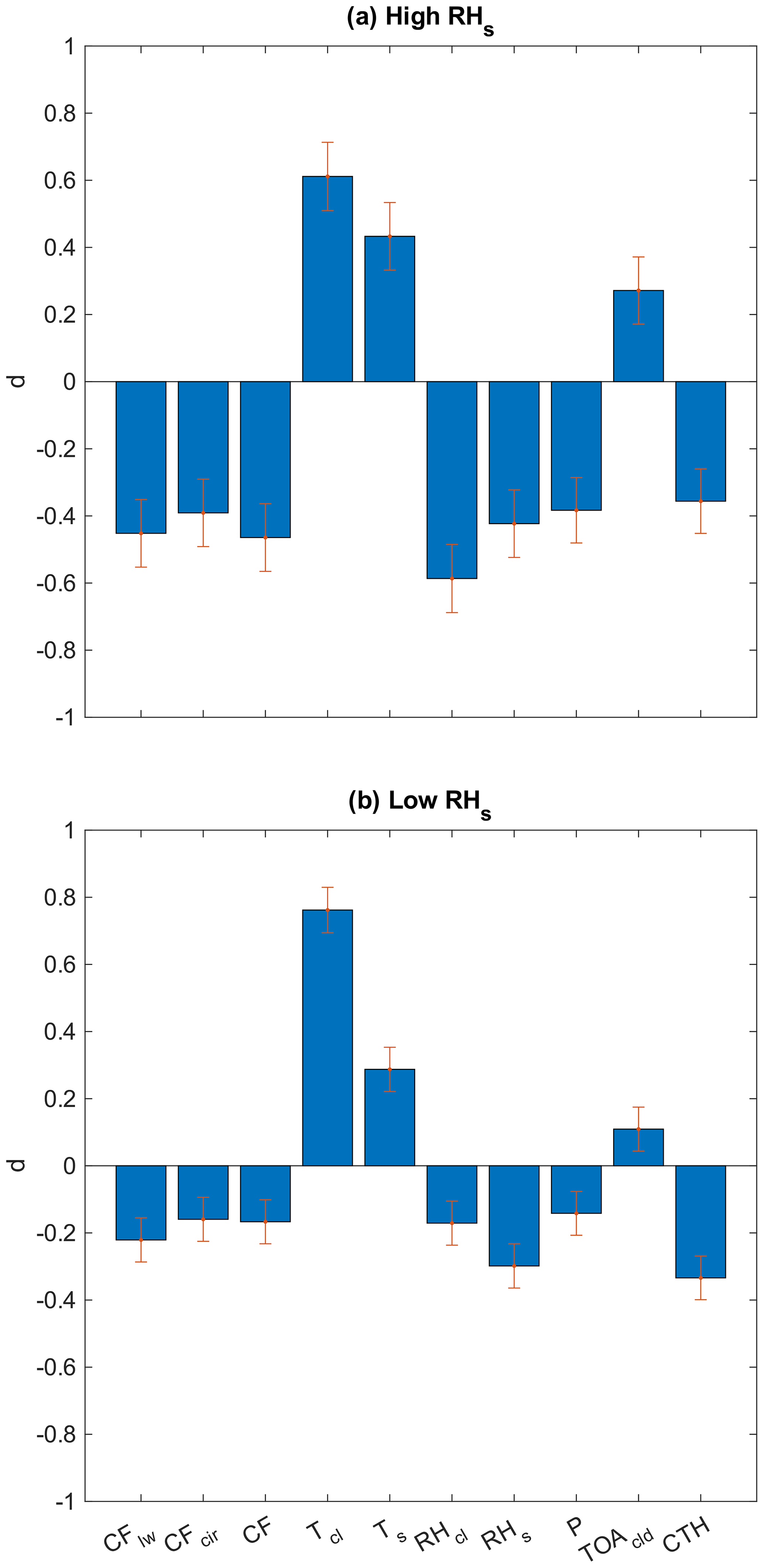
Figure 14Effect size of large fires in nCA on the mean of various meteorological variables during the fire season of 2003–2022 June–October. Cohen's d values for the difference between nCA-NV regional averages of variables on high DM days minus low nCA DM emission days that coincide with (a) high RHs and (b) low RHs. For Cohen's d, values of 0.2–0.5 signify a weak effect size, values of 0.5–0.8 represent a moderate effect size, and values greater or equal to 0.8 signify a strong effect size. Red bars represent standard error.
4.5 Cloud microphysical effects
Up to this point, we have investigated how cloud fraction and type differ during large fires. Aerosols from wildfires may also influence clouds via microphysical effects, which are investigated in this section. High fire emissions under high RHs conditions are associated with non-significant differences in microphysical variables (Fig. 15). Spatial maps of high minus low fire Reff and LWP under high RHs conditions show a mix of areas with positive and negative changes, most of which are not significant (Fig. S12). Although there is a small tendency for negative Reff anomalies to occur in Nevada and a small tendency for negative LWP anomalies to occur in nCA and western NV. Since negative Reff anomalies can affect precipitation, the spatial distribution of Reff anomalies (Figs. S12, S13) was compared with the spatial distribution of P anomalies (Figs. 13, S11) under high vs. low DM conditions. Significant negative Reff anomalies were not found to be spatially consistent with significant negative P anomalies under either high or low RHs conditions. This casts doubt on wildfires in this region creating microphysical suppression of P.
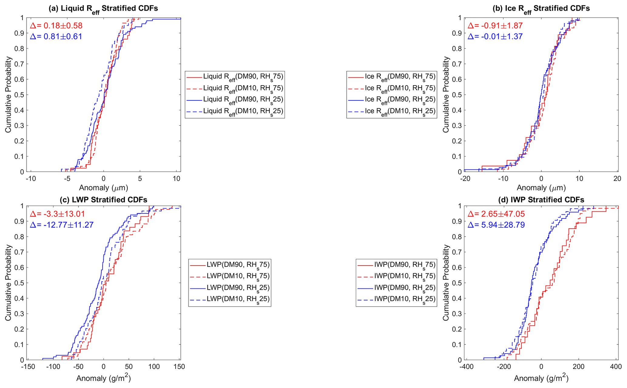
Figure 15Dependence of microphysical variables on high versus low surface relative humidity RHs and fires during the fire season. Empirical CDFs for regional average daily anomalies of cloud microphysical variables over the nCA-NV region during the 2003–2022 June–October period. Solid red line signifies variable anomalies stratified by (DM90, RHs75). The dashed red line signifies variable anomalies stratified by (DM10, RHs75). The solid blue line represents variable anomalies stratified (DM90, RHs25). The dashed blue line symbolizes variable anomalies stratified by (DM10, RHs25). Variables depicted include (a) liquid effective radius Reff, (b) ice Reff, (c) liquid water path LWP, and (d) ice water path IWP. The red Δ represents the differences in the mean of the solid red and dashed red lines (DM90, RHs75)−(DM10, RHs75). The blue Δ represents the differences in the mean of the solid blue and dashed blue lines (DM90, RHs25)−(DM10, RHs25).
There are significant regional changes in liquid Reff and LWP under low RHs conditions (Figs. 15, S13). Liquid Reff significantly increases under these conditions, which is contrary to what one would expect as a response to increased AOD (Twohy et al., 2021; Conrick et al., 2021; Fan et al., 2016). One possible explanation for this increase in Reff is that Reff is directly proportional to temperature (Martins et al., 2011), and perhaps the effects of the TCL anomalies dominate over the condensation of new droplets onto BCphi. Alternatively, this increase may be driven by changes in atmospheric dynamics, as increased updraft strength and enhanced turbulence could lead to increased coalescence (Khain, 2009). Coincident with the strongest increase in Reff (at the northernmost coast of California) under these conditions is a significant negative (upward) pressure velocity anomaly from 1000 to 925 hPa, which implies that an increase in upward convection near the surface may be a factor of the increase in Reff, as an upward pressure velocity should increase droplet lifetime (Fig. S14). It is also noted that there are negative pressure velocity anomalies under high RHs conditions from 1000 to 850 hPa (Fig. S15), and this corresponds to an increase in Reff near the Bay Area.
Comparing high with low fire conditions, LWP under simultaneously low RHs conditions shows a significant decrease (Fig. 15c). This significant negative LWP anomaly may be due to the negative RHCL anomaly (Fig. S11b), as lower saturation of the air would reduce liquid water within clouds. This decrease in LWP may be of importance, as LWP scales positively with cloud albedo (Han et al., 1998). Therefore, this decrease in LWP may contribute to an increase in absorbed solar radiation at the surface. In summary, while the nCA fires significantly inject aerosols into the troposphere, these aerosols do not appear to generally act as CCN and instead contribute to a positive T anomaly that burns off clouds. This may be because BC is generally more hydrophobic than other aerosols, and instead the radiative effects of the aerosol dominate.
The results of this paper indicate that large fires in nCA are concurrent with significant amounts of absorbing aerosols, which themselves are associated with a shortwave heating rate of 0.041 ± 0.016 to 0.093 ± 0.019 K d−1. This heating rate contributes to positive atmospheric T anomalies in the region that are concurrent with large fires; however, the extent of this contribution is unknown. When the fires occur during high RHs conditions, the positive T anomalies (Figs. 8, 13a) are associated with significant negative RH anomalies in the low, middle, and high cloud layers (850–300 hPa) at the 90 % confidence interval (Figs. 10, 13b). These negative RH anomalies are associated with a reduction in clouds, which is associated with significant negative P anomalies in the nCA-NV region. These negative CF anomalies are also associated with an increase in TOA radiative flux (Fig. 13h), despite a decrease in CTH (Fig. 13f). In short, wildfires in nCA are associated with region-wide negative CF anomalies that are caused by positive T anomalies. Aerosols emitted from biomass burning contribute to these positive T anomalies through shortwave absorption, indicating that the traditionally defined aerosol–cloud semi-direct effect is a possible explanation for the decrease in clouds. Furthermore, the TCL, RHCL, and CF anomalies correlate significantly with positive BC and AOD anomalies (Figs. 7, 8, 10, 11, and 13), further supporting the assertion that aerosols are contributing to these anomalies. However, it is unknown to what extent the aerosols contribute to the atmospheric T anomalies observed and therefore to the negative RH, CF, and P anomalies. One possible source of noise is wind. Figure S9 depicts a positive wind speed in northern Nevada that may be influencing cloud cover over that part of the region, and it is unknown whether this signal has anything to do with the positive T anomalies. Additionally, wildfires are associated with an increase in sensible heat flux from the combustion of biofuels, which may contribute to the positive T anomalies as well (Dickinson et al., 2021). Furthermore, random weather variations within the stratification may also create anomalies that are favorable for enhanced fire activity, which would increase DM, making causality difficult to discern. However, another study that utilized a similar methodology to this paper to analyze the effects of large fires using combined aircraft observations and a climate model indicates the possibility that the aerosols in this study are a significant contributor to the negative CF anomalies (Thornhill et al., 2018). The authors of that study ran the Met Office Unified Model using aircraft observations of AOD and BB aerosol properties. They compared meteorological variables in high vs. low fire emission conditions over South America and found a clear-sky shortwave heating rate of the low to middle troposphere that is larger than (0.2 K d−1), but comparable to, the heating rates calculated in this paper. This was also associated with a higher BC mass mixing ratio, and a significant negative CF anomaly of around 0.08, which is a similar anomaly to the 0.07 ± 0.05 MODIS CF anomaly observed in this study during high RHs conditions (Fig. 12c). Although not related to fire, an aircraft observational study of anthropogenic BC over the Bay of Bengal found a BC heating rate of around 0.5 K d−1 (Kant et al., 2023), which further demonstrates that BC can be associated with atmospheric warming. Furthermore, the results of this study are consistent with numerous other satellite observational studies over the tropics and subtropics that demonstrate that aerosols associated with wildfires are shortwave absorbing and can contribute to burn-off of clouds, resulting in a positive radiative forcing (Wilcox, 2012; Kaufman et al., 2005; Ackerman et al., 2000; Hansen et al., 1997). Additionally, the reduction in CF and P is consistent with the results of the study by Chen et al. (2014), which was a biomass burning modeling experiment conducted over the United States. However, their proposed mechanism for these decreases was a change in convection due to the distribution of warming of the aerosols. Concerning the increase in above sites of fire emission in Fig. 9b and c, this is consistent with a recent study by Yu et al. that found comparable results (Yu et al., 2024); however, they found more water vapor higher in the troposphere than this paper. Additionally, it is noted that the observed microphysical effects of the BB aerosols in this paper, namely, the lack of a regional decrease in Reff, are in contrast to another observational study that overlaps with the region of interest in this paper (Twohy et al., 2021). An important note about that study, however, is that it only sampled the 2018 wildfire season while this study focuses on the entire 2003–2022 period.
The results of this paper highlight that it is necessary to understand the contribution of biomass burning aerosols to the anomalies that favor enhanced fire weather. If the aerosols are a significant contributor to these anomalies, this can create a positive feedback loop where large fires emit copious amounts of BC, warm the atmosphere, reduce cloud cover, suppress P, and therefore intensify fire activity. As this potential feedback would prolong wildfires, it would therefore also prolong poor air quality conditions inside the southwestern US (Liu and Peng, 2019; O’Neill et al., 2021; Schlosser et al., 2017) as well as other parts of the country (Hung et al., 2020). Significant reductions in nCA P may prolong the wildfire season further into autumn (Goss et al., 2020), and increases in atmospheric T as well as decreases in atmospheric RH may create conditions more favorable for more fires to ignite and grow (Varga et al., 2022). Additionally, the negative P anomalies and/or positive Ts anomalies in this paper occur in heavily populated regions in the southwestern US, including the San Francisco Bay Area, Humboldt County in California, and Washoe County in Nevada. Therefore, it is essential to further investigate the relationship between anomalously large fires in the region and the local meteorology, since if the fires are contributing to these meteorological anomalies, this would dictate an increased need for a curtailment of CO2 emissions (Ma et al., 2021; Touma et al., 2021) and better land management practices (DellaSala et al., 2022; Minnich et al., 2000; Minnich, 2001), as climate change and land mismanagement have both contributed to the large fires in nCA in recent years. Additionally, the confirmation that these BC anomalies are associated with a positive heating rate anomaly is enough to advocate for these changes, as the fires are worsening already warm western US weather. Furthermore, as large fires are projected to become more commonplace throughout the 21st century due to these factors (Flannigan et al., 2013; United Nations Environment Programme, 2022), the results of this paper will become more relevant over time as today's 90th percentile fire emission conditions become more common throughout the 21st century.
Overall, to determine whether the fires are significantly contributing to the negative RH, CF, and P anomalies, it is essential to run a climate modeling experiment where BC is increased over the region of interest and to quantify the effects of this increased BC on these meteorological variables.
Table A1Definition of variables that were derived from satellite observational datasets as well as the instrument and dataset they are derived from.
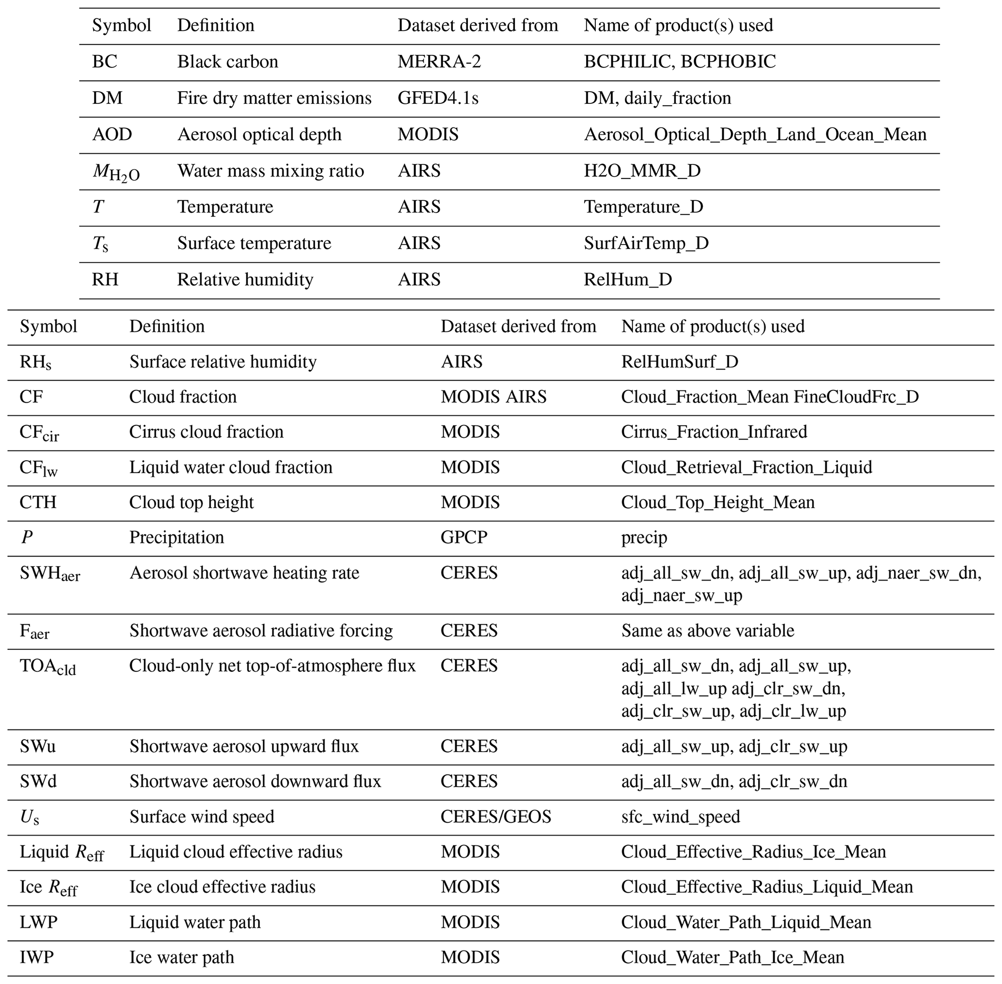
Table A2Definitions of abbreviations used throughout the paper that are not associated with a dataset.
Table A3Definitions of subscripts and other descriptors for variables.
Code is available upon request from the authors.
All datasets utilized in this analysis are available online for free. The MODIS–Aqua MYD08_D3 dataset can be found at the NASA Level-1 and Atmosphere Archive & Distribution System (LAADS) Distributed Active Archive Center (DAAC) (https://doi.org/10.5067/MODIS/MYD08_D3.061, MODIS Atmosphere Science Team, 2017). The AIRS–Aqua AIRS3STD dataset can also be accessed through the Goddard Earth Sciences Data and Information Services Center (GES DISC) (https://doi.org/10.5067/AQUA/AIRS/DATA303, AIRS Science Team and Texeira, 2013). The CERES Level 3 SYN1DEG-DAY dataset can also be found at LAADS DAAC (https://doi.org/10.5067/Terra+Aqua/CERES/SYN1degDay_L3.004A, NASA/LARC/SD/ASDC, 2017). The M2I3NVAER dataset can also be found at GES DISC (https://doi.org/10.5067/LTVB4GPCOTK2, Global Modeling And Assimilation Office and Pawson, 2015). GFED4.1s fire emissions data can be found at https://www.globalfiredata.org (GFED, 2024), or on the Oak Ridge National Laboratory (ORNL) DAAC (https://doi.org/10.3334/ORNLDAAC/1293, Randerson et al., 2017).
The supplement related to this article is available online at: https://doi.org/10.5194/acp-24-6937-2024-supplement.
JLG conceived the project, designed the study, performed the data analysis, and wrote the paper. RJA performed analyses and wrote the paper. KFL advised on methods.
The contact author has declared that none of the authors has any competing interests.
Publisher’s note: Copernicus Publications remains neutral with regard to jurisdictional claims made in the text, published maps, institutional affiliations, or any other geographical representation in this paper. While Copernicus Publications makes every effort to include appropriate place names, the final responsibility lies with the authors.
This research has been supported by the National Science Foundation (NSF; grant no. AGS-2153486 to Robert J. Allen).
This paper was edited by Matthew Christensen and reviewed by Michael Diamond and one anonymous referee.
Abel, S. J., Highwood, E. J., Haywood, J. M., and Stringer, M. A.: The direct radiative effect of biomass burning aerosols over southern Africa, Atmos. Chem. Phys., 5, 1999–2018, https://doi.org/10.5194/acp-5-1999-2005, 2005. a
Ackerman, A. S., Toon, O. B., Stevens, D. E., Heymsfield, A. J., Ramanathan, V., and Welton, E. J.: Reduction of Tropical Cloudiness by Soot, Science, 288, 1042–1047, https://doi.org/10.1126/science.288.5468.1042, 2000. a
Adler, R. F., Sapiano, M. R. P., Huffman, G. J., Wang, J.-J., Gu, G., Bolvin, D., Chiu, L., Schneider, U., Becker, A., Nelkin, E., Xie, P., Ferraro, R., and Shin, D.-B.: The Global Precipitation Climatology Project (GPCP) Monthly Analysis (New Version 2.3) and a Review of 2017 Global Precipitation, Atmosphere, 9, 138, https://doi.org/10.3390/atmos9040138, 2018. a
Ager, A. A., Day, M. A., Alcasena, F. J., Evers, C. R., Short, K. C., and Grenfell, I.: Predicting Paradise: Modeling future wildfire disasters in the western US, Sci. Total Environ., 784, 147057, https://doi.org/10.1016/j.scitotenv.2021.147057, 2021. a
AIRS Science Team and Texeira, J.: Aqua AIRS Level 3 Standard Daily Product using AIRS IR-only V6, Goddard Earth Sciences Data and Information Services Center (GES DISC) [data set], Greenbelt, MD, USA, https://doi.org/10.5067/AQUA/AIRS/DATA303, 2013. a, b
Allen, R. J. and Sherwood, S. C.: Aerosol-cloud semi-direct effect and land-sea temperature contrast in a GCM, Geophys. Res. Lett., 37, L07702, https://doi.org/10.1029/2010GL042759, 2010. a, b
Allen, R. J., Hassan, T., Randles, C. A., and Su, H.: Enhanced land–sea warming contrast elevates aerosol pollution in a warmer world, Nat. Clim. Change, 9, 300–305, https://doi.org/10.1038/s41558-019-0401-4, 2019. a, b
Allen, R. J., Zhao, X., Randles, C. A., Kramer, R. J., Samset, B. H., and Smith, C. J.: Surface warming and wetting due to methane’s long-wave radiative effects muted by short-wave absorption, Nat. Geosci., 16, 314–320, https://doi.org/10.1038/s41561-023-01144-z, 2023. a
Allen, R. J., Gomez, J., Horowitz, L. W., and Shevliakova, E.: Enhanced future vegetation growth with elevated carbon dioxide concentrations could increase fire activity, Communications Earth & Environment, 5, 1–15, https://doi.org/10.1038/s43247-024-01228-7, 2024a. a
Allen, R. J., Vega, C., Yao, E., and Liu, W.: Impact of industrial versus biomass burning aerosols on the Atlantic Meridional Overturning Circulation, npj Climate and Atmospheric Science, 7, 1–16, https://doi.org/10.1038/s41612-024-00602-8, 2024b. a
Amiri-Farahani, A., Allen, R. J., Neubauer, D., and Lohmann, U.: Impact of Saharan dust on North Atlantic marine stratocumulus clouds: importance of the semidirect effect, Atmos. Chem. Phys., 17, 6305–6322, https://doi.org/10.5194/acp-17-6305-2017, 2017. a
Amiri-Farahani, A., Allen, R. J., Li, K.-F., Nabat, P., and Westervelt, D. M.: A La Niña-Like Climate Response to South African Biomass Burning Aerosol in CESM Simulations, J. Geophys. Res.-Atmos., 125, e2019JD031832, https://doi.org/10.1029/2019JD031832, 2020. a
Artaxo, P., Rizzo, L. V., Brito, J. F., Barbosa, H. M. J., Arana, A., Sena, E. T., Cirino, G. G., Bastos, W., Martin, S. T., and Andreae, M. O.: Atmospheric aerosols in Amazonia and land use change: from natural biogenic to biomass burning conditions, Faraday Discuss., 165, 203–235, https://doi.org/10.1039/c3fd00052d, 2013. a
Brown, P. T., Hanley, H., Mahesh, A., Reed, C., Strenfel, S. J., Davis, S. J., Kochanski, A. K., and Clements, C. B.: Climate warming increases extreme daily wildfire growth risk in California, Nature, 621, 760–766, https://doi.org/10.1038/s41586-023-06444-3, 2023. a
Buchard, V., da Silva, A. M., Colarco, P. R., Darmenov, A., Randles, C. A., Govindaraju, R., Torres, O., Campbell, J., and Spurr, R.: Using the OMI aerosol index and absorption aerosol optical depth to evaluate the NASA MERRA Aerosol Reanalysis, Atmos. Chem. Phys., 15, 5743–5760, https://doi.org/10.5194/acp-15-5743-2015, 2015. a, b
Cape, J. N., Coyle, M., and Dumitrean, P.: The atmospheric lifetime of black carbon, Atmos. Environ., 59, 256–263, https://doi.org/10.1016/j.atmosenv.2012.05.030, 2012. a
Chen, D., Liu, Z., Schwartz, C. S., Lin, H.-C., Cetola, J. D., Gu, Y., and Xue, L.: The impact of aerosol optical depth assimilation on aerosol forecasts and radiative effects during a wild fire event over the United States, Geosci. Model Dev., 7, 2709–2715, https://doi.org/10.5194/gmd-7-2709-2014, 2014. a, b
Chen, Y., Hall, J., van Wees, D., Andela, N., Hantson, S., Giglio, L., van der Werf, G. R., Morton, D. C., and Randerson, J. T.: Multi-decadal trends and variability in burned area from the fifth version of the Global Fire Emissions Database (GFED5), Earth Syst. Sci. Data, 15, 5227–5259, https://doi.org/10.5194/essd-15-5227-2023, 2023. a
Cho, C., Kim, S.-W., Choi, W., and Kim, M.-H.: Significant light absorption of brown carbon during the 2020 California wildfires, Sci. Total Environ., 813, 152453, https://doi.org/10.1016/j.scitotenv.2021.152453, 2022. a, b
Conrick, R., Mass, C. F., Boomgard-Zagrodnik, J. P., and Ovens, D.: The Influence of Wildfire Smoke on Cloud Microphysics during the September 2020 Pacific Northwest Wildfires, Weather Forecast., 36, 1519–1536, https://doi.org/10.1175/WAF-D-21-0044.1, 2021. a
DellaSala, D. A., Baker, B. C., Hanson, C. T., Ruediger, L., and Baker, W.: Have western USA fire suppression and megafire active management approaches become a contemporary Sisyphus?, Biol. Conserv., 268, 109499, https://doi.org/10.1016/j.biocon.2022.109499, 2022. a
Dickinson, M. B., Wold, C. E., Butler, B. W., Kremens, R. L., Jimenez, D., Sopko, P., and O'Brien, J. J.: The Wildland Fire Heat Budget—Using Bi-Directional Probes to Measure Sensible Heat Flux and Energy in Surface Fires, Sensors, 21, 2135, https://doi.org/10.3390/s21062135, 2021. a, b
Eyring, V., Bony, S., Meehl, G. A., Senior, C. A., Stevens, B., Stouffer, R. J., and Taylor, K. E.: Overview of the Coupled Model Intercomparison Project Phase 6 (CMIP6) experimental design and organization, Geosci. Model Dev., 9, 1937–1958, https://doi.org/10.5194/gmd-9-1937-2016, 2016. a
Fan, J., Wang, Y., Rosenfeld, D., and Liu, X.: Review of Aerosol–Cloud Interactions: Mechanisms, Significance, and Challenges, J. Atmos. Sci., 73, 4221–4252, https://doi.org/10.1175/JAS-D-16-0037.1, 2016. a
Fasullo, J. T., Rosenbloom, N., Buchholz, R. R., Danabasoglu, G., Lawrence, D. M., and Lamarque, J.-F.: Coupled Climate Responses to Recent Australian Wildfire and COVID-19 Emissions Anomalies Estimated in CESM2, Geophys. Res. Lett., 48, e2021GL093841, https://doi.org/10.1029/2021GL093841, 2021. a
Flannigan, M., Cantin, A. S., de Groot, W. J., Wotton, M., Newbery, A., and Gowman, L. M.: Global wildland fire season severity in the 21st century, Forest Ecol. Manag., 294, 54–61, https://doi.org/10.1016/j.foreco.2012.10.022, 2013. a
Ford, P. L. and Johnson, G. V.: Effects of dormant- vs. growing-season fire in shortgrass steppe: Biological soil crust and perennial grass responses, J. Arid Environ., 67, 1–14, https://doi.org/10.1016/j.jaridenv.2006.01.020, 2006. a
Giglio, L. and Justice, C.: MYD14A1 MODIS/Aqua Thermal Anomalies/Fire Daily L3 Global 1km SIN Grid V006, NASA EOSDIS Land Processes Distributed Active Archive Center [data set], https://doi.org/10.5067/MODIS/MYD14A1.006, 2015. a
Giglio, L., Randerson, J. T., and Van Der Werf, G. R.: Analysis of daily, monthly, and annual burned area using the fourth‐generation global fire emissions database (GFED4), J. Geophys. Res.-Biogeo., 118, 317–328, https://doi.org/10.1002/jgrg.20042, 2013. a
Giglio, L., Boschetti, L., Roy, D. P., Humber, M. L., and Justice, C. O.: The Collection 6 MODIS burned area mapping algorithm and product, Remote Sens. Environ., 217, 72–85, https://doi.org/10.1016/j.rse.2018.08.005, 2018. a
Global Fire Emissions Database (GFED): https://www.globalfiredata.org, last access: 4 May 2024. a
Global Modeling And Assimilation Office and Pawson, S.: MERRA-2 inst3_3d_aer_Nv: 3d,3-Hourly,Instantaneous,Model-Level,Assimilation,Aerosol Mixing Ratio V5.12.4, Goddard Earth Sciences Data and Information Services Center (GES DISC) [data set], Greenbelt, MD, USA, https://doi.org/10.5067/LTVB4GPCOTK2, 2015. a, b, c
Gomez, J., Allen, R. J., Turnock, S. T., Horowitz, L. W., Tsigaridis, K., Bauer, S. E., Olivié, D., Thomson, E. S., and Ginoux, P.: The projected future degradation in air quality is caused by more abundant natural aerosols in a warmer world, Communications Earth & Environment, 4, 1–11, https://doi.org/10.1038/s43247-023-00688-7, 2023. a
Goren, T. and Rosenfeld, D.: Satellite observations of ship emission induced transitions from broken to closed cell marine stratocumulus over large areas, J. Geophys. Res.-Atmos., 117, D17206, https://doi.org/10.1029/2012JD017981, 2012. a
Goss, M., Swain, D. L., Abatzoglou, J. T., Sarhadi, A., Kolden, C. A., Williams, A. P., and Diffenbaugh, N. S.: Climate change is increasing the likelihood of extreme autumn wildfire conditions across California, Environ. Res. Lett., 15, 094016, https://doi.org/10.1088/1748-9326/ab83a7, 2020. a
Han, Q., Rossow, W. B., Chou, J., and Welch, R. M.: Global Survey of the Relationships of Cloud Albedo and Liquid Water Path with Droplet Size Using ISCCP, J. Climate, 11, 1516–1528, https://doi.org/10.1175/1520-0442(1998)011<1516:GSOTRO>2.0.CO;2, 1998. a
Hansen, J., Sato, M., and Ruedy, R.: Radiative forcing and climate response, J. Geophys. Res.-Atmos., 102, 6831–6864, https://doi.org/10.1029/96JD03436, 1997. a
He, C., Li, Q., Liou, K.-N., Qi, L., Tao, S., and Schwarz, J. P.: Microphysics-based black carbon aging in a global CTM: constraints from HIPPO observations and implications for global black carbon budget, Atmos. Chem. Phys., 16, 3077–3098, https://doi.org/10.5194/acp-16-3077-2016, 2016. a
Helmert, J., Heinold, B., Tegen, I., Hellmuth, O., and Wendisch, M.: On the direct and semidirect effects of Saharan dust over Europe: A modeling study, J. Geophys. Res.-Atmos., 112, D13208, https://doi.org/10.1029/2006JD007444, 2007. a
Herbert, R. and Stier, P.: Satellite observations of smoke–cloud–radiation interactions over the Amazon rainforest, Atmos. Chem. Phys., 23, 4595–4616, https://doi.org/10.5194/acp-23-4595-2023, 2023. a, b
Highwood, E. J. and Ryder, C. L.: Radiative Effects of Dust, in: Mineral Dust: A Key Player in the Earth System, edited by: Knippertz, P. and Stuut, J.-B. W., Springer Netherlands, Dordrecht, 267–286, https://doi.org/10.1007/978-94-017-8978-3_11, ISBN 978-94-017-8978-3, 2014. a
Huffman, G. J., Adler, R. F., Morrissey, M. M., Bolvin, D. T., Curtis, S., Joyce, R., McGavock, B., and Susskind, J.: Globa Precipitation at One-Degree Daily Resolution from Multisatellite Observations, J. Hydrometeorol., 2, 36–50, https://doi.org/10.1175/1525-7541(2001)002<0036:GPAODD>2.0.CO;2, 2001. a
Hung, W.-T., Lu, C.-H. S., Shrestha, B., Lin, H.-C., Lin, C.-A., Grogan, D., Hong, J., Ahmadov, R., James, E., and Joseph, E.: The impacts of transported wildfire smoke aerosols on surface air quality in New York State: A case study in summer 2018, Atmos. Environ., 227, 117415, https://doi.org/10.1016/j.atmosenv.2020.117415, 2020. a
Jacobson, M. Z.: Effects of biomass burning on climate, accounting for heat and moisture fluxes, black and brown carbon, and cloud absorption effects, J. Geophys. Res.-Atmos., 119, 8980–9002, https://doi.org/10.1002/2014JD021861, 2014. a
Kant, S., Sarangi, C., and Wilcox, E. M.: Aerosol processes perturb cloud trends over Bay of Bengal: observational evidence, npj Climate and Atmospheric Science, 6, 1–8, https://doi.org/10.1038/s41612-023-00443-x, 2023. a
Kaufman, Y. J., Koren, I., Remer, L. A., Rosenfeld, D., and Rudich, Y.: The effect of smoke, dust, and pollution aerosol on shallow cloud development over the Atlantic Ocean, P. Natl. Acad. Sci. USA, 102, 11207–11212, https://doi.org/10.1073/pnas.0505191102, 2005. a
Keeley, J. E. and Syphard, A. D.: Twenty-first century California, USA, wildfires: fuel-dominated vs. wind-dominated fires, Fire Ecol., 15, 24, https://doi.org/10.1186/s42408-019-0041-0, 2019. a
Khain, A. P.: Notes on state-of-the-art investigations of aerosol effects on precipitation: a critical review, Environ. Res. Lett., 4, 015004, https://doi.org/10.1088/1748-9326/4/1/015004, 2009. a, b
Koch, D. and Del Genio, A. D.: Black carbon semi-direct effects on cloud cover: review and synthesis, Atmos. Chem. Phys., 10, 7685–7696, https://doi.org/10.5194/acp-10-7685-2010, 2010. a
Kok, J. F., Storelvmo, T., Karydis, V. A., Adebiyi, A. A., Mahowald, N. M., Evan, A. T., He, C., and Leung, D. M.: Mineral dust aerosol impacts on global climate and climate change, Nature Reviews Earth & Environment, 4, 71–86, https://doi.org/10.1038/s43017-022-00379-5, 2023. a
LeNoir, J. S., McConnell, L. L., Fellers, G. M., Cahill, T. M., and Seiber, J. N.: Summertime transport of current-use pesticides from California's Central Valley to the Sierra Nevada Mountain Range, USA, Environ. Toxicol. Chem., 18, 2715–2722, https://doi.org/10.1002/etc.5620181210, 1999. a
Levy, R. C., Mattoo, S., Munchak, L. A., Remer, L. A., Sayer, A. M., Patadia, F., and Hsu, N. C.: The Collection 6 MODIS aerosol products over land and ocean, Atmos. Meas. Tech., 6, 2989–3034, https://doi.org/10.5194/amt-6-2989-2013, 2013. a
Li, F., Val Martin, M., Andreae, M. O., Arneth, A., Hantson, S., Kaiser, J. W., Lasslop, G., Yue, C., Bachelet, D., Forrest, M., Kluzek, E., Liu, X., Mangeon, S., Melton, J. R., Ward, D. S., Darmenov, A., Hickler, T., Ichoku, C., Magi, B. I., Sitch, S., van der Werf, G. R., Wiedinmyer, C., and Rabin, S. S.: Historical (1700–2012) global multi-model estimates of the fire emissions from the Fire Modeling Intercomparison Project (FireMIP), Atmos. Chem. Phys., 19, 12545–12567, https://doi.org/10.5194/acp-19-12545-2019, 2019. a, b
Li, S. and Banerjee, T.: Spatial and temporal pattern of wildfires in California from 2000 to 2019, Scientific Reports, 11, 8779, https://doi.org/10.1038/s41598-021-88131-9, 2021. a, b
Liu, J. C. and Peng, R. D.: The impact of wildfire smoke on compositions of fine particulate matter by ecoregion in the Western US, J. Expo. Sci. Env. Epid., 29, 765–776, https://doi.org/10.1038/s41370-018-0064-7, 2019. a
Liu, Z., Hu, M., Hu, Y., and Wang, G.: Estimation of net primary productivity of forests by modified CASA models and remotely sensed data, Int. J. Remote Sens., 39, 1092–1116, https://doi.org/10.1080/01431161.2017.1381352, 2018. a
Lohmann, U., Friebel, F., Kanji, Z. A., Mahrt, F., Mensah, A. A., and Neubauer, D.: Future warming exacerbated by aged-soot effect on cloud formation, Nat. Geosci., 13, 674–680, https://doi.org/10.1038/s41561-020-0631-0, 2020. a, b
Ma, W., Zhai, L., Pivovaroff, A., Shuman, J., Buotte, P., Ding, J., Christoffersen, B., Knox, R., Moritz, M., Fisher, R. A., Koven, C. D., Kueppers, L., and Xu, C.: Assessing climate change impacts on live fuel moisture and wildfire risk using a hydrodynamic vegetation model, Biogeosciences, 18, 4005–4020, https://doi.org/10.5194/bg-18-4005-2021, 2021. a
Mangeon, S., Voulgarakis, A., Gilham, R., Harper, A., Sitch, S., and Folberth, G.: INFERNO: a fire and emissions scheme for the UK Met Office's Unified Model, Geosci. Model Dev., 9, 2685–2700, https://doi.org/10.5194/gmd-9-2685-2016, 2016. a
Martins, J. V., Marshak, A., Remer, L. A., Rosenfeld, D., Kaufman, Y. J., Fernandez-Borda, R., Koren, I., Correia, A. L., Zubko, V., and Artaxo, P.: Remote sensing the vertical profile of cloud droplet effective radius, thermodynamic phase, and temperature, Atmos. Chem. Phys., 11, 9485–9501, https://doi.org/10.5194/acp-11-9485-2011, 2011. a
Minnich, R. A.: An Integrated Model of Two Fire Regimes, Conserv. Biol., 15, 1549–1553, https://doi.org/10.1046/j.1523-1739.2001.01067.x, 2001. a
Minnich, R. A. and Chou, Y. H.: Wildland Fire Patch Dynamics in the Chaparral of Southern California and Northern Baja California, Int. J. Wildland Fire, 7, 221–248, https://doi.org/10.1071/wf9970221, 1997. a
Minnich, R. A., Barbour, M. G., Burk, J. H., and Sosa-Ramírez, J.: Californian mixed-conifer forests under unmanaged fire regimes in the Sierra San Pedro Mártir, Baja California, Mexico, J. Biogeogr., 27, 105–129, https://doi.org/10.1046/j.1365-2699.2000.00368.x, 2000. a
MODIS Atmosphere Science Team: MYD08_D3 MODIS/Aqua Aerosol Cloud Water Vapor Ozone Daily L3 Global 1Deg CMG, NASA MODIS Adaptive Processing System, Goddard Space Flight Center [data set], USA, https://doi.org/10.5067/MODIS/MYD08_D3.061, 2017. a, b
NASA/LARC/SD/ASDC: CERES Time-Interpolated TOA Fluxes, Clouds and Aerosols Daily Aqua Edition4A, NASA Langley Atmospheric Science Data Center DAAC [data set], https://doi.org/10.5067/AQUA/CERES/SSF1DEGDAY_L3.004A, 2015. a
NASA/LARC/SD/ASDC: CERES and GEO-Enhanced TOA, Within-Atmosphere and Surface Fluxes, Clouds and Aerosols Daily Terra-Aqua Edition4A, NASA Langley Atmospheric Science Data Center DAAC [data set], https://doi.org/10.5067/Terra+Aqua/CERES/SYN1degDay_L3.004A, 2017. a, b
NASA/LARC/SD/ASDC: CERES and GEO-Enhanced TOA, Within-Atmosphere and Surface Fluxes, Clouds and Aerosols Daily Terra-NOAA20 Edition4A, NASA Langley Atmospheric Science Data Center DAAC [data set], https://doi.org/10.5067/Terra-NOAA20/CERES/SYN1degDay_L3.004A, 2023. a
Nguyen, L. S. P., Huang, H.-Y., Lei, T. L., Bui, T. T., Wang, S.-H., Chi, K. H., Sheu, G.-R., Lee, C.-T., Ou-Yang, C.-F., and Lin, N.-H.: Characterizing a landmark biomass-burning event and its implication for aging processes during long-range transport, Atmos. Environ., 241, 117766, https://doi.org/10.1016/j.atmosenv.2020.117766, 2020. a
Ogren, J. A. and Charlson, R. J.: Elemental carbon in the atmosphere: cycle and lifetime, Tellus B, 35B, 241–254, https://doi.org/10.1111/j.1600-0889.1983.tb00027.x, 1983. a
O’Neill, S. M., Diao, M., Raffuse, S., Al-Hamdan, M., Barik, M., Jia, Y., Reid, S., Zou, Y., Tong, D., West, J. J., Wilkins, J., Marsha, A., Freedman, F., Vargo, J., Larkin, N. K., Alvarado, E., and Loesche, P.: A multi-analysis approach for estimating regional health impacts from the 2017 Northern California wildfires, J. Air Waste Manage., 71, 791–814, https://doi.org/10.1080/10962247.2021.1891994, 2021. a
Palinkas, L. A.: The California Wildfires, in: Global Climate Change, Population Displacement, and Public Health: The Next Wave of Migration, edited by: Palinkas, L. A., Springer International Publishing, Cham, 53–67, https://doi.org/10.1007/978-3-030-41890-8_4, ISBN 978-3-030-41890-8, 2020. a
Peng, J., Hu, M., Guo, S., Du, Z., Zheng, J., Shang, D., Levy Zamora, M., Zeng, L., Shao, M., Wu, Y.-S., Zheng, J., Wang, Y., Glen, C. R., Collins, D. R., Molina, M. J., and Zhang, R.: Markedly enhanced absorption and direct radiative forcing of black carbon under polluted urban environments, P. Natl. Acad. Sci. USA, 113, 4266–4271, https://doi.org/10.1073/pnas.1602310113, 2016. a
Peterson, D., Wang, J., Ichoku, C., Hyer, E., and Ambrosia, V.: A sub-pixel-based calculation of fire radiative power from MODIS observations: 1: Algorithm development and initial assessment, Remote Sens. Environ., 129, 262–279, https://doi.org/10.1016/j.rse.2012.10.036, 2013. a
Platnick, S., King, M., Ackerman, S., Menzel, W., Baum, B., Riedi, J., and Frey, R.: The MODIS cloud products: algorithms and examples from Terra, IEEE T. Geosci. Remote, Sensing, 41, 459–473, https://doi.org/10.1109/TGRS.2002.808301, 2003. a
Platnick, S., Meyer, K. G., King, M. D., Wind, G., Amarasinghe, N., Marchant, B., Arnold, G. T., Zhang, Z., Hubanks, P. A., Holz, R. E., Yang, P., Ridgway, W. L., and Riedi, J.: The MODIS Cloud Optical and Microphysical Products: Collection 6 Updates and Examples From Terra and Aqua, IEEE T. Geosci. Remote, 55, 502–525, https://doi.org/10.1109/TGRS.2016.2610522, 2017. a
Raga, G. B., Baumgardner, D., Rios, B., Díaz-Esteban, Y., Jaramillo, A., Gallagher, M., Sauvage, B., Wolff, P., and Lloyd, G.: High concentrations of ice crystals in upper-tropospheric tropical clouds: is there a link to biomass and fossil fuel combustion?, Atmos. Chem. Phys., 22, 2269–2292, https://doi.org/10.5194/acp-22-2269-2022, 2022. a
Randerson, J., van der Werf, G., Giglio, L., Collatz, G., and Kasibhatla, P.: Global Fire Emissions Database, Version 4.1 (GFEDv4), p. 1925.7122549999906 MB, ORNL DAAC, Oak Ridge, Tennessee, USA, https://doi.org/10.3334/ORNLDAAC/1293, 2017. a, b
Randles, C. A., Silva, A. M. d., Buchard, V., Colarco, P. R., Darmenov, A., Govindaraju, R., Smirnov, A., Holben, B., Ferrare, R., Hair, J., Shinozuka, Y., and Flynn, C. J.: The MERRA-2 Aerosol Reanalysis, 1980 Onward. Part I: System Description and Data Assimilation Evaluation, J. Climate, 30, 6823–6850, https://doi.org/10.1175/JCLI-D-16-0609.1, 2017. a
Ruffault, J., Curt, T., Moron, V., Trigo, R. M., Mouillot, F., Koutsias, N., Pimont, F., Martin-StPaul, N., Barbero, R., Dupuy, J.-L., Russo, A., and Belhadj-Khedher, C.: Increased likelihood of heat-induced large wildfires in the Mediterranean Basin, Scientific Reports, 10, 13790, https://doi.org/10.1038/s41598-020-70069-z, 2020. a
Sakaeda, N., Wood, R., and Rasch, P. J.: Direct and semidirect aerosol effects of southern African biomass burning aerosol, J. Geophys. Res.-Atmos., 116, D12205, https://doi.org/10.1029/2010JD015540, 2011. a
Salomonson, V., Barnes, W., Xiong, J., Kempler, S., and Masuoka, E.: An overview of the Earth Observing System MODIS instrument and associated data systems performance, in: IEEE International Geoscience and Remote Sensing Symposium, Toronto, ON, Canada, 24–28 June 2002, IEEE, 2, 1174–1176, https://doi.org/10.1109/IGARSS.2002.1025812, 2002. a
Samset, B. H.: Aerosol absorption has an underappreciated role in historical precipitation change, Communications Earth & Environment, 3, 1–8, https://doi.org/10.1038/s43247-022-00576-6, 2022. a
Sand, M., Samset, B. H., Tsigaridis, K., Bauer, S. E., and Myhre, G.: Black Carbon and Precipitation: An Energetics Perspective, J. Geophys. Res.-Atmos., 125, e2019JD032239, https://doi.org/10.1029/2019JD032239, 2020. a
Schlosser, J. S., Braun, R. A., Bradley, T., Dadashazar, H., MacDonald, A. B., Aldhaif, A. A., Aghdam, M. A., Mardi, A. H., Xian, P., and Sorooshian, A.: Analysis of aerosol composition data for western United States wildfires between 2005 and 2015: Dust emissions, chloride depletion, and most enhanced aerosol constituents, J. Geophys. Res.-Atmos., 122, 8951–8966, https://doi.org/10.1002/2017JD026547, 2017. a, b
Shi, G., Yan, H., Zhang, W., Dodson, J., Heijnis, H., and Burrows, M.: Rapid warming has resulted in more wildfires in northeastern Australia, Sci. Total Environ., 771, 144888, https://doi.org/10.1016/j.scitotenv.2020.144888, 2021. a
Smith, C. J., Kramer, R. J., Myhre, G., Forster, P. M., Soden, B. J., Andrews, T., Boucher, O., Faluvegi, G., Fläschner, D., Hodnebrog, Ø., Kasoar, M., Kharin, V., Kirkevåg, A., Lamarque, J.-F., Mülmenstädt, J., Olivié, D., Richardson, T., Samset, B. H., Shindell, D., Stier, P., Takemura, T., Voulgarakis, A., and Watson-Parris, D.: Understanding Rapid Adjustments to Diverse Forcing Agents, Geophys. Res. Lett., 45, 12023–12031, https://doi.org/10.1029/2018GL079826, 2018. a
Stjern, C. W., Samset, B. H., Myhre, G., Forster, P. M., Hodnebrog, Ø., Andrews, T., Boucher, O., Faluvegi, G., Iversen, T., Kasoar, M., Kharin, V., Kirkevåg, A., Lamarque, J.-F., Olivié, D., Richardson, T., Shawki, D., Shindell, D., Smith, C. J., Takemura, T., and Voulgarakis, A.: Rapid Adjustments Cause Weak Surface Temperature Response to Increased Black Carbon Concentrations, J. Geophys. Res.-Atmos., 122, 11462–11481, https://doi.org/10.1002/2017JD027326, 2017. a
Thornhill, G. D., Ryder, C. L., Highwood, E. J., Shaffrey, L. C., and Johnson, B. T.: The effect of South American biomass burning aerosol emissions on the regional climate, Atmos. Chem. Phys., 18, 5321–5342, https://doi.org/10.5194/acp-18-5321-2018, 2018. a, b
Touma, D., Stevenson, S., Lehner, F., and Coats, S.: Human-driven greenhouse gas and aerosol emissions cause distinct regional impacts on extreme fire weather, Nat. Commun., 12, 212, https://doi.org/10.1038/s41467-020-20570-w, 2021. a
Tsikerdekis, A., Zanis, P., Georgoulias, A. K., Alexandri, G., Katragkou, E., Karacostas, T., and Solmon, F.: Direct and semi-direct radiative effect of North African dust in present and future regional climate simulations, Clim. Dynam., 53, 4311–4336, https://doi.org/10.1007/s00382-019-04788-z, 2019. a
Twohy, C. H., Toohey, D. W., Levin, E. J. T., DeMott, P. J., Rainwater, B., Garofalo, L. A., Pothier, M. A., Farmer, D. K., Kreidenweis, S. M., Pokhrel, R. P., Murphy, S. M., Reeves, J. M., Moore, K. A., and Fischer, E. V.: Biomass Burning Smoke and Its Influence on Clouds Over the Western U. S., Geophys. Res. Lett., 48, e2021GL094224, https://doi.org/10.1029/2021GL094224, 2021. a, b, c, d
United Nations Environment Programme: Spreading like Wildfire – The Rising Threat of Extraordinary Landscape Fires, A UNEP Rapid Response Assessment, Nairobi, https://www.unep.org/resources/report/spreading-wildfire-rising-threat-extraordinary-landscape-fires (last access: 4 May 2024), 2022. a, b, c
Urbanski, S. P.: Combustion efficiency and emission factors for wildfire-season fires in mixed conifer forests of the northern Rocky Mountains, US, Atmos. Chem. Phys., 13, 7241–7262, https://doi.org/10.5194/acp-13-7241-2013, 2013. a
Urbanski, S. P., Hao, W. M., and Nordgren, B.: The wildland fire emission inventory: western United States emission estimates and an evaluation of uncertainty, Atmos. Chem. Phys., 11, 12973–13000, https://doi.org/10.5194/acp-11-12973-2011, 2011. a
van der Werf, G. R., Randerson, J. T., Giglio, L., van Leeuwen, T. T., Chen, Y., Rogers, B. M., Mu, M., van Marle, M. J. E., Morton, D. C., Collatz, G. J., Yokelson, R. J., and Kasibhatla, P. S.: Global fire emissions estimates during 1997–2016, Earth Syst. Sci. Data, 9, 697–720, https://doi.org/10.5194/essd-9-697-2017, 2017. a, b, c
Varga, K., Jones, C., Trugman, A., Carvalho, L. M. V., McLoughlin, N., Seto, D., Thompson, C., and Daum, K.: Megafires in a Warming World: What Wildfire Risk Factors Led to California’s Largest Recorded Wildfire, Fire, 5, 16, https://doi.org/10.3390/fire5010016, 2022. a, b, c
Wagenbrenner, N. S., Germino, M. J., Lamb, B. K., Robichaud, P. R., and Foltz, R. B.: Wind erosion from a sagebrush steppe burned by wildfire: Measurements of PM10 and total horizontal sediment flux, Aeolian Res., 10, 25–36, https://doi.org/10.1016/j.aeolia.2012.10.003, 2013. a
Wagenbrenner, N. S., Chung, S. H., and Lamb, B. K.: A large source of dust missing in Particulate Matter emission inventories? Wind erosion of post-fire landscapes, Elementa: Science of the Anthropocene, 5, 2, https://doi.org/10.1525/elementa.185, 2017. a
Wagner, R., Jähn, M., and Schepanski, K.: Wildfires as a source of airborne mineral dust – revisiting a conceptual model using large-eddy simulation (LES), Atmos. Chem. Phys., 18, 11863–11884, https://doi.org/10.5194/acp-18-11863-2018, 2018. a
Wagner, R., Schepanski, K., and Klose, M.: The dust emission potential of agricultural-like fires – Theoretical estimates from two conceptually different dust emission parameterizations, J. Geophys. Res.-Atmos., 126, e2020JD034355, https://doi.org/10.1029/2020JD034355, 2021. a
Wei, J., Li, Z., Peng, Y., and Sun, L.: MODIS Collection 6.1 aerosol optical depth products over land and ocean: validation and comparison, Atmos. Environ., 201, 428–440, https://doi.org/10.1016/j.atmosenv.2018.12.004, 2019. a
Wilcox, E. M.: Direct and semi-direct radiative forcing of smoke aerosols over clouds, Atmos. Chem. Phys., 12, 139–149, https://doi.org/10.5194/acp-12-139-2012, 2012. a
Wilmot, T. Y., Mallia, D. V., Hallar, A. G., and Lin, J. C.: Wildfire plumes in the Western US are reaching greater heights and injecting more aerosols aloft as wildfire activity intensifies, Scientific Reports, 12, 12400, https://doi.org/10.1038/s41598-022-16607-3, 2022. a, b
Wu, C., Wu, D., and Yu, J. Z.: Quantifying black carbon light absorption enhancement with a novel statistical approach, Atmos. Chem. Phys., 18, 289–309, https://doi.org/10.5194/acp-18-289-2018, 2018. a
Yu, J., Jiang, X., Zeng, Z.-C., and Yung, Y. L.: Fire monitoring and detection using brightness-temperature difference and water vapor emission from the atmospheric infrared sounder, J. Quant. Spectrosc. Ra., 317, 108930, https://doi.org/10.1016/j.jqsrt.2024.108930, 2024. a, b
Yu, Y. and Ginoux, P.: Enhanced dust emission following large wildfires due to vegetation disturbance, Nat. Geosci., 15, 878–884, https://doi.org/10.1038/s41561-022-01046-6, 2022. a
Zaremba, L. L. and Carroll, J. J.: Summer Wind Flow Regimes over the Sacramento Valley, J. Appl. Meteorol. Clim., 38, 1463–1473, https://doi.org/10.1175/1520-0450(1999)038<1463:SWFROT>2.0.CO;2, 1999. a